Robert Brignall
A Thesis Submitted for the Degree of PhD
at the
University of St. Andrews
2007
Full metadata for this item is available in the St Andrews
Digital Research Repository
at:
https://research-repository.st-andrews.ac.uk/
Please use this identifier to cite or link to this item:
http://hdl.handle.net/10023/431
This item is protected by original copyright
This item is licensed under a
S
IMPLICITY IN
R
ELATIONAL
S
TRUCTURES AND
ITS
APPLICATION TO
P
ERMUTATION
CLASSES
R
OBERTBRIGNALL
D
ECLARATIONS
I Robert Brignall hereby certify that this thesis, which is approximately 40,000 words, has been written by me, that it is a record of work carried out by me, and that it has not been submitted in any previous application for a higher degree.
Signed: Date:
I was admitted as a research student in September 2004 and as a candidate for the degree of PhD in September 2004; the higher investigation of which this is a record was carried out in the University of St Andrews between September 2004 and July 2007.
Signed: Date:
I hereby certify that the candidate has fulfilled the conditions of the Resolution and Reg-ulations appropriate for the degree of Ph.D. in the University of St Andrews and that the candidate is qualified to submit this thesis in application to that degree.
Signature of Supervisor: Date:
In submitting this thesis to the University of St Andrews I understand that I am giving permission for it to be made available in accordance with the regulations of the University Library for the time being in force, subject to any copyright vested in the work not being affected thereby. I also understand that the title and abstract will be published, and that a copy of the work may be supplied to any bona fide library or research worker, that my thesis will be electronically available for personal or research use, and that the library has the right to migrate my thesis into new electronic forms as required to ensure continued access to the thesis. I have obtained any third-party copyright permissions that may be required in order to allow such access and migration.
A
CKNOWLEDGEMENTS
I would like to thank my supervisor, Nik Ruˇskuc, for introducing me to the area of per-mutation patterns and for his support throughout this process. Additionally, particular thanks go to Vince Vatter for the many hours of fruitful discussions we have had, and without whom this thesis would be very different and almost certainly less rewarding.
Thanks must also go to my various other collaborators – Sophie Huczynska, Mike Atkin-son and Michael Albert – for their time, and to Steve Waton and Steve Linton for their contributions to my knowledge of the area. Also, the anonymous referees of the papers on which this thesis is based have provided enriching comments.
To those with whom I have shared an office – Nelson Silva, Steve Waton, Andreas Dis-tler and Victor Maltcev – thanks for making my time here enjoyable. I am also grateful to the many staff and students of the School of Mathematics and Statistics for their support and friendship, and to countless other friends and acquaintances both in St Andrews and elsewhere.
This thesis has been greatly enhanced by the music of J.S. Bach.
Final thanks, however, must go to my parents, my grandparents, brother and sister, and to Gwen, for her unending support, company and patience.
I acknowledge generous funding from EPSRC.
A
BSTRACT
The simple relational structures form the units, or atoms, upon which all other relational structures are constructed by means of the substitution decomposition. This decomposi-tion appears to have first been introduced in 1953 in a talk by Fra¨ıss´e, though it did not appear in an article until a paper by Gallai in 1967. It has subsequently been frequently rediscovered from a wide variety of perspectives, ranging from game theory to combina-torial optimization.
Of all the relational structures — a set which also includes graphs, tournaments and posets — permutations are receiving ever increasing amounts of attention. A simple per-mutationis one that maps every nontrivial contiguous set of indices to a set of indices that is never contiguous. Simple permutations and intervals of permutations are important in biomathematics, while permutation classes — downsets under the pattern containment order — arise naturally in settings ranging from sorting to algebraic geometry.
We begin by studying simple permutations themselves, though always aim to estab-lish this theory within the broader context of relational structures. We first develop the technology of “pin sequences”, and prove that every sufficiently long simple permutation must contain either a long horizontal or parallel alternation, or a long pin sequence. This gives rise to a simpler unavoidable substructures result, namely that every sufficiently long simple permutation contains a long alternation or oscillation.
Erd˝os, Fried, Hajnal and Milner showed in 1972 that every tournament could be ex-tended to a simple tournament by adding at most two additional points. We prove analo-gous results for permutations, graphs, and posets, noting that in these three cases we may need to extend a structure by adding d(n+ 1)/2e points in the case of permutations and
posets, andlog2(n+ 1)points in the graph case.
The importance of simple permutations in permutation classes has been well estab-lished in recent years. We extend this knowledge in a variety of ways, first by showing that, in a permutation class containing only finitely many simple permutations, every sub-set defined by properties belonging to a finite “query-complete sub-set” is enumerated by an algebraic generating function. Such properties include being an even or alternating per-mutation, or avoiding generalised (blocked or barred) permutations. We further indicate that membership of a permutation class containing only finitely many simple permuta-tions can be computed in linear time.
Using the decomposition of simple permutations, we establish, by representing pin se-quences as a language over an eight-letter alphabet, that it is decidable if a permutation class given by a finite basis contains only finitely many simple permutations. We also dis-cuss possible approaches to the same question for other relational structures, in particular the difficulties that arise for graphs. The pin sequence technology provides a further result relating to the wreath product of two permutation classes, namely thatCoDis finitely based
wheneverDdoes not admit arbitrarily long pin sequences. As a partial converse, we also
C
ONTENTS
Declarations i
Acknowledgements iii
Abstract v
Introduction xi
Part I Simplicity 1
1 Preliminaries 3
1.1 Permutations, Containment and Order Isomorphism . . . 4
1.2 Graphical Representation and Symmetries . . . 5
1.3 Relational Structures . . . 7
1.4 Intervals and Simplicity . . . 8
1.4.1 Interacting Intervals . . . 11
1.4.2 Asymptotics . . . 12
1.5 Inflations and the Substitution Decomposition . . . 15
1.5.1 The Permutation Case . . . 17
2 Decomposition 21 2.1 Background . . . 21
2.2 Pin Sequences . . . 23
2.3 Simple Permutations without Long Proper Pin Sequences. . . 28
2.4 Pin Words . . . 34
2.5 Unavoidable Substructures in Simple Permutations . . . 39
2.6 Other Contexts . . . 41
2.6.1 Pin Sequences in Graphs. . . 41
3 Simple Extensions 47 3.1 Introduction . . . 47
3.2 Permutations . . . 48
3.3 Graphs . . . 52
3.4 Tournaments. . . 56
3.5 Posets . . . 59
4 Substitution Decomposition Algorithms 65 4.1 One- and Three-sided Intervals . . . 66
4.2 Generating Intervals . . . 71
4.3 Strong Intervals and the Substitution Decomposition . . . 73
4.4 Graph Substitution Decomposition . . . 77
Part II Permutation Classes 79 5 Containment as a Partial Order 81 5.1 Defining Permutation Classes . . . 82
5.1.1 Examples . . . 83
5.1.2 New Classes from Old . . . 86
5.2 Enumeration . . . 91
5.3 Antichains, Partial Well Order and Atomicity . . . 95
5.3.1 Partial Well Order . . . 98
5.3.2 Atomicity . . . 101
CONTENTS ix
5.4.1 Finitely Many Simples . . . 105
5.5 The Containment Partial Order in Other Structures . . . 107
6 Algebraic Generating Functions 111 6.1 Introduction . . . 111
6.2 Properties and Query-completeness . . . 112
6.3 Proof of Main Result . . . 113
6.4 Finite Query-Complete Sets . . . 116
6.5 Examples . . . 121
6.6 Involutions . . . 123
6.7 Cyclic Closures . . . 126
6.8 Applicability and Application . . . 130
6.8.1 Simple Decomposition Revisited . . . 132
6.8.2 Linear Time Membership . . . 134
7 Decidability and Unavoidable Substructures 137 7.1 Introduction . . . 137
7.2 The Easy Decisions . . . 139
7.3 Review of Regular Languages and Automata . . . 143
7.4 Decidability . . . 145
7.5 An Easier Sufficient Condition . . . 150
7.6 Other Contexts. . . 151
7.7 The Pin Class . . . 153
8 The Wreath Product 155 8.1 D-Profiles . . . 156
8.2 The Minimal Block . . . 159
8.3 Pin Sequences and the Wreath Product . . . 162
8.4 Infinitely Based Examples . . . 164
Bibliography 171
I
NTRODUCTION
This thesis consists of two parts: In Part Iwe study the structure of simple permutations in the context of relational structures, while in Part IIwe apply this structural knowledge of simplicity to permutation classes. This division reflects the fact that the study of per-mutations — and particularly simple perper-mutations — lies in an area of research extending beyond the subject of permutation classes. However, that these two topics are covered un-der the single title of this thesis reflects the importance in studying simple permutations for the further understanding of permutation classes. Many of the major permutation-based results in this thesis may be found published or available as preprints [28,29,30,31].
In Chapter1 we begin by introducing permutations and the containment partial or-der. We then take a more broad view by defining the general construction of relational structures, and demonstrate how permutations, graphs, tournaments and posets may all be described in this language. We then commence our discussion in Sections1.4and1.5of intervals, simplicity and the substitution decomposition in the context of relational struc-tures, at each stage also translating back to the permutation case.
In Chapter 2we introduce the new technology of pin sequences and show how suf-ficiently long simple permutations must contain either a long proper pin sequence, or a long wedge or parallel alternation. We also introduce the language of pins, a necessary prerequisite for the decidability result of Chapter7. We close the chapter with a specula-tive discussion on possible analogues of this decomposition theory for graphs.
Motivated by a result of Erd˝os, Fried, Hajnal and Milner in 1972 for tournaments, Chapter3considers the problem of embedding a given relational structure inside a larger simple structure. We demonstrate that a general approach may be used relying on the
stitution decomposition, but that the outcome for each type of relational structure may be somewhat unique. To demonstrate this, we look at the simple extensions of permutations, graphs, tournaments and posets.
Much emphasis has been placed in recent years in developing optimal algorithms for computing intervals and the substitution decomposition. In Chapter4we review a recent paper by Bergeron, Chauve, Montgolfier and Raffinot who give a linear-time algorithm to compute the intervals in a given permutation. It follows directly from this work that the permutation substitution decomposition may be computed in linear time. We also review some algorithmic results in the case of graphs.
Permutation classes have been intensively studied in recent years, and in Chapter 5
we review some of the results in this area, manifested primarily in constructions between permutation classes, their enumeration and special properties including partial well order and atomicity. Permutation classes containing only finitely many simple permutations have received particular attention, and we cover the most important results concerning these.
One particular property of permutation classes containing only finitely many simple permutations is that they are enumerated by algebraic generating functions. By means of “finite query-complete sets of properties”, we show in Chapter6that many different sub-sets of such permutation classes are also enumerated by algebraic generating functions. We close the chapter with some further enumerative results coming from the decomposi-tion of simple permutadecomposi-tions in Chapter2, and note how, using the linear-time substitution decomposition algorithm of Chapter 4, we may establish in linear time whether a given permutation lies in a specified class known to contain only finitely many simple permuta-tions.
INTRODUCTION xiii
language, and hence its infinitude is decidable.
PART
I
C
HAPTER
1
P
RELIMINARIES
E
XPRESSING an object in terms of smaller, indecomposable objects, is a goal aimed at ina wide variety of subject areas. The first example one finds in mathematics is the Fun-damental Theorem of Arithmetic, which demonstrates how any positive integer greater than 1 may be written uniquely (up to ordering) as a product of prime factors. It is a property that is not true for elements of an arbitrary collection, however; take for exam-ple the elements of a ring, which in general are not uniquely factorisable (unless the ring is specifically shown to be a Unique Factorisation Domain). When a given collection of objects can be uniquely factorised, emphasis is often placed on the study of the prime or indecomposable elements, as it is these which form the “building blocks” of the collection. One such family of objects is the family of relational structures – objects governed by a given set of relations – whose most notable members include graphs, tournaments, per-mutations and posets. Their “factorisation” is relatively straightforward, and will be re-ferred to as the “substitution decomposition”, though is known also as the modular de-composition, disjunctive decomposition andX-join. The elemental building blocks of this
decomposition are the “simple” structures. This term is used primarily in the context of permutations, while in other contexts these structures are called prime or indecomposable (note in particular that “simple” usually has a different meaning in the context of graphs). The notion of substitution decomposition dates back at least to a 1953 talk of Fra¨ıss´e, but only the abstract of this talk [55] survives. The first article using the substitution de-composition seems to be Gallai [58] (for an English translation, see [59]), who applied them
particularly to the study of transitive orientations of graphs. Some work on the substitu-tion decomposisubstitu-tion in the general context can be found in M¨ohring [92]. It has proved to be a useful technique in a wide variety of settings, ranging from game theory to combi-natorial optimisation (see M¨ohring [94] or M¨ohring and Radermacher [95] for extensive references).
Our relational structure of choice is the permutation. It has sufficient complexity to be worthy of extended study, but also is easily represented graphically. In this setting, much of the motivation for studying the substitution decomposition is for the purposes of enumeration, particularly of permutation classes, and Part IIis primarily dedicated to demonstrating the enumerative consequences of this study.
Adapting the permutation-specific theory we will develop to other relational struc-tures is not necessarily obvious; much of the theory depends, as we have indicated, on the graphical representation of permutations, and so, for example, finding a graph-theoretic analogue will not follow immediately. Thus throughout Part Iwe will discuss the success (or otherwise) of existing attempts in this avenue.
1.1 Permutations, Containment and Order Isomorphism
We begin by introducing the terms we need to study permutations; the definition of a general relational structure will follow after this is established. For n ∈ Ndenote by[n] the set{1,2, . . . , n}, and fori ≤ j let[i, j]correspond to the set{i, i+ 1, . . . , j}. We may
sometimes also refer to open or half-open segments, for example(i, j]denotes the set{i+ 1, i+ 2, . . . , j}.
In our context, a permutation π of length nis an ordering of the elements of [n]. For example, π = 918572364is a permutation of length9. Two particular families of permu-tations to which we will refer relatively often are the increasing permutations denoted by
ιn= 12· · ·n, and thedecreasing permutationsδn=n(n−1)· · ·1.
1.2 GRAPHICALREPRESENTATION ANDSYMMETRIES 5
and in this pair i is the position and π(i) the value of the point. Viewing π as a set of
points immediately indicates the graphical interpretation which will prove invaluable in our forthcoming study. We will, however, postpone this viewpoint momentarily while we introduce some further definitions.
Two finite sequences of the same length,α = a1a2· · ·an andβ = b1b2· · ·bn, are said
to be order isomorphicif, for all i, j, we haveai < aj if and only ifbi < bj. As such, each
sequence of distinct real numbers is order isomorphic to a unique permutation. For a sequenceα and set of permutationsC, with a slight abuse of notation we will sometimes
write statements like “α∈ C”, meaning “the permutation order isomorphic toαlies inC.”.
Similarly, any given subsequence (or pattern) of a permutationπ is order isomorphic to a
smaller permutation, σ say, and such a subsequence is called acopy of σ in π. We may
also say thatπ containsσ (or, in some texts,πinvolvesσ) and writeσ ≤π. If, on the other
hand,πdoes not contain a copy of some givenσ, thenπis said toavoidσ. For example,π= 918572346containsσ = 51342because of the subsequence91572(=π(1)π(2)π(4)π(5)π(6)), but avoidsτ = 3142.
The pattern containment order forms a partial order on the set of all permutations, and in PartIIwe will be looking at sets of permutations closed under taking subpermutations. A book introducing the study of these permutation patterns has been written by B´ona [22].
1.2 Graphical Representation and Symmetries
As mentioned above, we may think of a permutation π as a set of points (i, π(i)), and immediately we can form a graphical representation. We can go further, however, and give a pictorial description of order isomorphism. Two setsSandT of points in the plane
are said to be order isomorphic if the axes can be stretched and shrunk in some manner to map one of the sets onto the other, i.e., if there are strictly increasing functionsf, g:R→R such that{(f(s1), g(s2)) : (s1, s2)∈S}=T. (As the inverse of a strictly increasing function is also strictly increasing, this is an equivalence relation.)
Figure 1.1:The plot of the permutationπ= 934826715.
plane in which no two points share a coordinate (often called a genericor noncorectilinear
set) is order isomorphic to the plot of a unique permutation; in practice we will simply say that a point set is order isomorphic to a permutation. See Figure1.1for an example. Steve Waton’s PhD thesis [118] extends this graphical interpretation of containment to consider the sets of permutations that can be drawn by taking points lying on a given geometrical shape.
This geometric viewpoint indicates several of the symmetries of pattern containment. The maps(x, y) 7→ (−x, y),(x, y) 7→ (x,−y)and(x, y) 7→ (y, x), when applied to generic point sets, correspond to “reversing”, “complementing” and “inverting” permutations re-spectively. Formally, thereverseof a permutationπof lengthnis the permutation obtained
by reading the sequence of symbols ofπ in reverse order, i.e. from right to left. For each i∈[n], theith component of thecomplementofπ is assigned valuen+ 1−π(i), while the
inverseofπ is denotedπ−1 and is defined byπ−1(j) =i, wherej=π(i). For example, the reverse ofπ= 934826715is517628439, its complement is176284395andπ−1= 852396741.
1.3 RELATIONAL STRUCTURES 7
1.3 Relational Structures
The most general objects we will consider are the relational structures, which we now introduce as a precursor to handling simplicity and the substitution decomposition. For any setA, ak-ary relationR is a subset ofAk. An ordered sequence of relations overAis
then called arelational structure.
More specifically, define a relational language, L, to be a set ofrelational symbols R
to-gether with positive integersnRdenoting the arity of the symbolsR. A relational structure
Awhose relational symbols are those ofLis then defined by itsground setdom(A)and a set of subsets RA ⊆ dom(A)nR for each R ∈ L. Such a structure will also be called an
L-structure. If, for example,(a1, . . . , anR) ∈RA then we writeRA(a1, . . . , anR), andRA is
annR-ary relation.
We will be working primarily with relational structures whose ground sets are finite, though many of these principles may be applied to infinite relational structures. In partic-ular, the substitution decomposition is readily extended to include infinite structures, as shown in [95].
We now briefly review how some well-known objects may be viewed as relational structures.
Permutations. A permutationπ on npoints may be viewed as the relational structure
Aπ with ground setdom(Aπ) = [n], on a language containing two binary linear relations,
L = {<,≺, n< = 2, n≺ = 2}. The first relation,<Aπ, is the normal ordering on[n], while
i≺Aπ jif and only ifπ(i)< π(j). For example,π= 934826715corresponds to the relational
structureAπon[9]with
1<2<3<4<5<6<7<8<9
and
Graphs. A graphGis a relational structureAGon the languageL={E, nE = 2}, where E is a binary symmetric relation, dom(AG) = V(G), andEAG(x, y) if and only ifx ∼ y
in G. The analogue to containment in graphs is the notion of theinduced subgraph:1 an
induced subgraph ofGis a graph formed on any subset of vertices fromG, withx∼yin
the subgraph if and only ifx∼yinG.
Tournaments. A tournament is a complete oriented graph. A tournament T therefore
corresponds to the relational structureAT on the languageL = {→, n→ = 2}, but where
→ is now a trichotomous binary relation, i.e. for eachx, y ∈ dom(AT) = V(T), precisely
one ofx =y,x →AT y ory →AT xis true. The name “tournament” derives from its use
to denote a competition where every pair of playersx, ymust meet each other in a match,
the outcome being either that x wins, denoted y → x, or that x loses, denotedx → y.
The containment order on tournaments is not surprisingly the same as graphs; aninduced subtournament of a tournamentT is a tournament formed on any subset of vertices ofT
withx→yin the subtournament if and only ifx→yinT.
Posets. By definition, a poset is a relational structure on the language containing a single binary relation,<, which is reflexive, antisymmetric and transitive. Thecomparability graph G(P, <)of a poset(P, <)is a graph with vertex setP, and edgep∼q if and only if either
p < q orq < p. Conversely, ifGis a comparability graph for some poset(P, <), then the order<is called atransitive orientationof (the edges of)G. This connection between posets
and graphs arises in a number of combinatorial problems – see M¨ohring [93] for a survey.
1.4 Intervals and Simplicity
Before we can discuss the substitution decomposition, we must first define how we can find “factors” of a given relational structure, and hence define the elemental relational structures – those structures with no nontrivial factors.
1.4 INTERVALS ANDSIMPLICITY 9
Following F¨oldes [54], we say that a setX ⊆dom(A)is anintervalif for everyR ∈ L
andnR-tuple(x1, . . . , xnR)∈dom(A)nR \XnR, with at least onexi ∈X, then
RA(x1, . . . , xnR) ⇐⇒ RA(x1, . . . , xi−1, y, xi+1, . . . , xnR)for ally∈X.
Informally, an interval corresponds to a subsetXof the ground setdom(A)for which every pair of elements of X have exactly the same relations with the elements ofdom(A)\X.
Accordingly, every singleton set{x} ⊆ dom(A)is an interval, as is all ofdom(A). Every other interval is said to be a proper interval, and a structure is simple if it has no proper intervals.
Simplicity has, to some extent, been studied for relational structures in general, for ex-ample, by F¨oldes [54] and Schmerl and Trotter [107]. Much greater attention has, however, been diverted to particular structures, the most pertinent of which we will now review.
Permutations. In the permutation case, anintervalofπcorresponds to a set of contiguous
indices I = [a, b] such that the set of values π(I) = {π(i) : i ∈ I} is also contiguous.
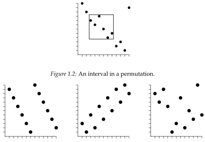
Intervals are clearly identified in the plot of a permutation as a set of points enclosed in an axis-parallel rectangle, with no points lying in the regions above, below, to the left or to the right (see Figure1.2for an example). Intervals of permutations are interesting in their own right and have applications to biomathematics, particularly to genetic algorithms for sequencing problems, and modelling the genomes of prokaryotes as permutations allows the matching of gene sequences.2 See Corteel, Louchard, and Pemantle [37] for extensive
references.
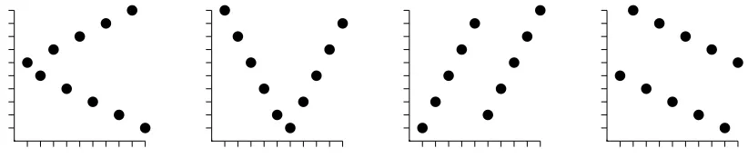
It then follows that asimple permutation is one whose only intervals are of length0,1 andn. Figure1.3shows three simple permutations of length12. Note that the eight order-isomorphism preserving symmetries also preserve intervals, and hence simplicity. The number of simple permutations of lengthn= 1,2, . . .is1,2,0,2,6,46,338,2926,28146, . . .
(sequence A111111 of [110]), the first few being1, 12, 21,2413 and3142. We will look at the asymptotics of this sequence in Subsection1.4.2.
2In these contexts, the term “common interval” is used, indicating a segment upon which two or more
Figure 1.2:An interval in a permutation.
Figure 1.3:The plots of three simple permutations of length12.
Graphs. An interval in a graph3 is a set of verticesX ⊆ V(G) such that N(v)\X = N(w)\X for allv, w∈X, whereN(v)denotes the neighbourhood ofvinG. A graph onn
vertices therefore has several trivial intervals (∅,V(G), and the singletons); a graph with no nontrivial intervals is then often called primeorindecomposable(the word simple meaning something completely different in this context). These graphs have been the subject of considerable study, see for example Ehrenfeucht, Harju, and Rozenberg [47], Ille [71], and Sabidussi [105]. A survey of indecomposability and the substitution decomposition in graphs can be found in Brandst¨adt, Le, and Spinrad [27].
Tournaments. An interval in a tournamentT is a setA ⊆V(T) such that for allv /∈ A,
eitherv→ Aorv ←A. Clearly the empty set, all singletons, and the entire vertex set are
all intervals ofT, andT is said to be simple if it has no others. Crvenkovi´c, Dolinka, and
Markovi´c [40] survey the algebraic and combinatorial results concerning simple
tourna-3These are also called autonomous sets, blocks, bound sets, clans, closed sets, clumps, committees,
1.4 INTERVALS ANDSIMPLICITY 11
ments.
Posets. An interval of a poset(P, <)corresponds to a setA⊆P which for everyp∈P\A
satisfies one ofp < A,p > Aorpis incomparable to every point ofA. Intervals in a poset
correspond to “convex” intervals in its related comparability graph. A subset ofB ⊆P is
called(P, <)-convexif the set{r ∈P : there existp, q∈B such thatp < r < q}is a subset
ofB. The following lemma is then easily deduced:
Lemma 1.1(Buer and M¨ohring [32]). Given a poset(P, <), the set of intervals of(P, <)is equal
to the set of(P, <)-convex intervals ofG(P, <).
1.4.1 Interacting Intervals
In the general context of relational structures, intervals interact with each other in a pleas-ing way. Two intervals are said tooverlapif neither interval is contained in the other and their intersection is nontrivial.
Proposition 1.2. For any two overlapping intervalsIandJof theL-structureA,
(a) I∩J is an interval ofA(F¨oldes [54, Proposition 1]),
(b) I∪J is an interval ofA(F¨oldes [54, Proposition 2]), and
(c) I\J is an interval ofA.
Proof. We will prove only Case (c) in the case whereLconsists solely of ak-ary relationR
(k≥2); the result for a general languageLfollows immediately. IfIandJare overlapping
intervals of A, we must show that if RA(x
1, x2, . . . , xk) with x1 ∈ I \ J and not all of
x2, . . . , xklie inI\J, thenRA(y, x2, . . . , xk)for anyy∈I\J.
SinceI is an interval and x1, y ∈ I, we are finished if, for some i ∈ [2, k], xi lies in dom(A)\I, so suppose that everyxi ∈I∩J. SinceIandJoverlap, there exists at least one
z∈J\I, and soRA(x1, x2, x3, . . . , xk)impliesRA(x1, z, x3, . . . , xk)becauseJis an interval.
We can now obtainRA(y, z, x
Figure 1.4:Two intervals and their intersection.
For two setsX and Y, letX4Y denote the symmetric difference of X andY, namely
(X∪Y)\(X∩Y). Providing a relational structureAis defined by a language consisting only of binary symmetric relations and relations with arity at least3, then the symmetric difference of two intersecting intervals is also an interval.
Proposition 1.3(M¨ohring and Radermacher [95, Theorem 4.1.1]). LetA be anL-structure
for which nR ≥ 2for every R ∈ L. Then if I and J are overlapping intervals, I4J is also an interval if every binary relationR∈ Lis symmetric.
In the permutation case, Proposition 1.3 clearly does not apply. However, Proposi-tion1.2is easily seen by considering the graphical representation, as in Figure1.4.
1.4.2 Asymptotics
The asymptotic enumeration of simple structures has been studied variously for permu-tations, tournaments, graphs, and indeed in a more general setting. We will presently review the problem for permutations and graphs, with a view to showing that although both these structures fall within the category of relational structures, the solutions are sig-nificantly different (although the approach is essentially identical). One the one hand, the dominant term in the asymptotic enumeration of simple permutations isn!/e2 (a fraction
1/e2 of the total number of permutations of lengthn), while on the other hand almost all
graphs are indecomposable.
1.4 INTERVALS ANDSIMPLICITY 13
the substitution decomposition), but many other results are only true in certain cases. We will encounter further differences as we progress through this study of simplicity – first in the difficulties of adapting the permutation-specific simple decomposition to the graph case in Chapter2, and then again in the widely varying bounds on simple extensions in Chapter3.
Graphs. Let us begin with the graph case, which turns out to be fairly straightforward. Let the random variableXkdenote the number of intervals of sizekin a random graphG
onnvertices. The probability that a given set ofkvertices is an interval is 2 n−k
2(n2)
, since each of then−kvertices outside the interval must look at every vertex inside the interval in the
same way. As there are n k
ways of choosing the set ofkvertices, we have
E[Xk] = n k
2n−k
2(n2) .
Thus the probability that G is decomposable may be bounded above by the sum of the
expected number of proper intervals, i.e. it is bounded byE[X2 +X3+· · ·+Xn−1]. By linearity of expectation, this yields
Pr(Gis decomposable)≤ 2
n
2(n2) n−1
X
k=2
n k
2k .
Observing that the sum is the binomial expansion of (1 + 12)nless the first two and final
terms, we obtain
Pr(Gis decomposable)≤ 2 n
2(n2)
3 2
n
−1−n 2 −
1 2n
→0asn→ ∞,
and hence almost all graphs are indecomposable. M¨ohring [91] shows this is also true for several other cases, including tournaments, posets and structures defined on single asym-metric relations. For the tournament version, see also Erd˝os, Fried, Hajnal and Milner [51].
Permutations. Proceeding as we did with graphs, let the random variableXkdenote the
values. The set of positions must begin at one of the firstn−k+ 1positions ofπ, and at the
same time the lowest point in the set of values must be one of the lowestn−k+ 1values of
π. Of the nk
sets of values to which the contiguous set of positions may be mapped, only one maps to the chosen contiguous set of values. Thus we have
E[Xk] =
(n−k+ 1)2 n k
=
(n−k+ 1)(n−k+ 1)!k!
n! .
Already we can see some difficulties may arise; whereas in the graph case it was clear that the denominator (being an exponential inn2) would always dominate the numerator,
here we see that this will not always hold. In particular, E[X2] = 2(nn−1) → 2 as n →
∞, implying in fact that, asymptotically, we expect to find two intervals of size two in a
random permutation. Seeking the asymptotics of the other terms innX−1 k=2
E[Xk], we consider
the casesk = 3,k = 4,k=n−2(assumingn≥4) andk=n−1separately:
E[X3] =
6(n−2)
n(n−1) ≤ 6
n →0
E[X4] =
4!(n−3)
n(n−1)(n−2) ≤ 24
n2 →0
E[Xn−2] =
3·3!
n(n−1) ≤ 24
n2 →0
E[Xn−1] =
4
n →0.
The remaining terms form a partial sum, which converges providing E[Xk+1]
E[Xk]
< 1. Sim-plifying this equation gives2k2−(3n+ 1)k+n2+n+ 1>0, a quadratic ink, which yields
two roots. The smaller of these satisfies0 < k− ≤n, the largerk+ > n. Thus fork ≤k−, E[Xk]is decreasing, while fork− < k < n,E[Xk] is increasing, and henceE[Xk] ≤ 24/n2
for4≤k ≤n−2. Thus
n−2
X
k=4
E[Xk]≤(n−5)24
n2 ≤
24
n →0.
Subsequently, the only term of
n−1
X
k=2
E[Xk]which is non-zero in the limitn → ∞ isk = 2.
Ignoring larger intervals, occurrences of intervals of size2in a random permutationπcan
1.5 INFLATIONS AND THESUBSTITUTIONDECOMPOSITION 15
the occurrence of any specific interval is relatively rare. Heuristically, this suggests that
X2 is asymptotically Poisson distributed with parameter2. Using this heuristic, we have Pr(X2 = 0) → e−2 asn → ∞, and so there are approximately en2! simple permutations of
lengthn.
A formal argument for this is implicitly given in Uno and Yagiura [116], and was made explicit by Corteel, Louchard, and Pemantle [37]. The method, however, essentially dates back to the 1940s with Kaplansky [74] and Wolfowitz [121], who considered “runs” within permutations – a runis a set of points with contiguous positions whose values arei, i+ 1, . . . , i+rori+r, i+r−1, . . . , i, in that order.4
A non-probabilistic approach (but one still relying on the work of Kaplansky) produc-ing more precise asymptotics is given by Albert, Atkinson, and Klazar [3]. They obtain the following theorem, and note that higher order terms are obtainable given sufficient computation:
Theorem 1.4(Albert, Atkinson and Klazar [3]). The number of simple permutations of length nis asymptotically given by
n!
e2
1− 4
n+
2
n(n−1) +O(n −3)
.
1.5 Inflations and the Substitution Decomposition
With the notion of simplicity established, we may now describe how all relational struc-tures can be decomposed and written in terms of these simple objects. This is easier to establish by first defining the reverse process. Given an L-structure S, an inflation of S
by the L-structures As for eachs ∈ dom(S)— denotedS[As : s ∈ dom(S)] — is theL
-structure obtained by replacing each elementsofdom(S)with a set of elementsdom(As)
that form an interval in theL-structureA=S[As:s∈dom(S)], i.e. for everyR∈ L:
RA(a1, . . . , anR)⇐⇒
RAs(a
1, . . . , anR)anda1, . . . , anR ∈dom(As),s∈dom(S), or RS(s
1, . . . , snR)where eachsi ∈dom(S)andai ∈ Asi.
4Atkinson and Stitt [12] called permutations containing no runsstrongly irreducible. Note that this is
Adeflation(ordecomposition) of anL-structureAis the reverse. We writeA=S[As:s∈ dom(S)]to mean any deflation ofAby disjoint intervalsAs. We are primarily interested
in the case whereS is simple – the following theorem gives the uniqueness of such anS,
which will be called theskeleton.
Theorem 1.5(The Substitution Decomposition). LetAbe anL-structure for some languageL.
Then there exists a unique simple L-structureS such thatA =S[As : s ∈ dom(S)]. Moreover, when|dom(S)|>2, everyAsis defined uniquely.
Proof. LetMdenote the set of all intervals, exceptdom(A), which are contained in no other proper intervals.
If two intervals I, J ∈ M intersect, then Proposition 1.2.(b) shows thatI ∪J is also
an interval, which, unless I ∪J = dom(A), contradicts the definition of M. If I ∪J = dom(A), then Proposition 1.2.(c) shows that J \I is an interval, so Acan be written as
the inflation of a two-elementL-structure, all of which are simple. IfA=S[As1,As2]and
A =T[At1,At2]are two different two-element decompositions, then we may assume that
inAwe haveAs1∩ At1 6=∅andAs2∩ At2 6=∅. Thus relations inSbetweens1ands2must
agree with the relations inAbetween elements of the disjoint intervalsAs1 andAs2. Since
As1 ∩ At1 ⊆ As1 andAs2 ∩ At2 ⊆ As2 are intervals, the relations between elements ofAs1
andAs2correspond to the relations between the elements ofAs1∩At1andAs2∩At2, which,
by a similar argument must correspond to the relations between the elements ofAt1 and
At2, and these are none other than the relations betweent1 andt2 of dom(T). Similarly,
relations involving justs1 (respectively,s2) correspond to relations involving justt1 (t2), and soSandT are isomorphic.
Otherwise, the sets inM partitiondom(A). For eachI ∈ M choose a representative xI ∈ I, and define the L-structure S on{xI} by A|{xI} = S. ClearlyA is the inflation of S by the structuresA|I forI ∈ M. The simplicity ofS follows from the observation
that if S contained a proper interval K, then S
xI∈KI would be a proper interval of A
contradicting the definition ofM. Furthermore, ifA = T[At : t ∈ dom(T)]for any other
1.5 INFLATIONS AND THESUBSTITUTIONDECOMPOSITION 17
interval inM.
The non-unique cases which occur when|dom(S)|= 2may be dealt with in a number of ways, some of which are specific to particular types of structure, as we will see later. In the general setting, however, we can still find a unique substructure ofAthat is essentially
from one of three groups.
Proposition 1.6 (M¨ohring and Radermacher [95, Theorems 3.4.3, 4.1.2 and 4.1.3]). IfAis
an L-structure whose skeletonS satisfies|dom(S)| = 2, then there exists a unique maximalL
-structureT for whichA =T[At : t∈ dom(T)]and, for everyR ∈ L,RT is linear, complete or empty.
Once we have established the substitution decompositionA = S[As : s ∈ dom(S)],
we may repeat the process on the substructures As for each s ∈ dom(S). Iterating this
decomposition, we may continue until we are left only with substructures on singleton ground sets. We may represent this iterated substitution decomposition as a rooted tree – thesubstitution decomposition tree. Each node corresponds to a substructure ofAwhose
ground set is an interval, with the root of the tree beingAand the leaves being the singleton
ground sets. For a given node with corresponding non-singleton structureA0, the children of A0 are the substructures A0
s in the decompositionA0 = S0[As0 : s ∈ dom(S)]. IfS is a
unique simple with|dom(S)| ≥4, label the node corresponding toA0 with the symbolP (short for “proper”); if the (binary) relations in the language of S are linear and all other
relations are complete or empty, label the node with the symbolL; if all the relations in the
language ofS are complete or empty, label the nodeD(short for “degenerate”).
1.5.1 The Permutation Case
Restricting our attention to the permutation case, the substitution decomposition is some-what easier to describe. Given a permutationσ of lengthmand nonempty permutations α1, . . . , αm, theinflation of σ by α1, . . . , αm – denotedσ[α1, . . . , αm] – is the permutation
obtained by replacing each entry σ(i) by an interval that is order isomorphic to αi. For
Figure 1.5:The plot of479832156, an inflation of2413.
any expression ofπas an inflationπ =σ[π1, π2, . . . , πm], and we will callσaskeletonofπ.
Theorem1.5then specialises to become:
Proposition 1.7(Albert and Atkinson [2]). Every permutation may be written as the inflation of a unique simple permutation. Moreover, ifπcan be written asσ[α1, . . . , αm]whereσis simple andm≥4, then theαis are unique.
The degenerate cases occur when a permutation can be written as an inflation of either 12or 21, and we may choose a unique decomposition in these cases in a variety of ways. The principal decomposition that we will use for the substitution decomposition, however, is as described in Proposition1.6.
The direct sum of two permutationsα and β is the inflation 12[α, β], and is usually denotedα⊕β. Similarly, theskew sumis the inflation21[α, β], and is denotedα β. The
direct sum operation acts as a dichotomy on the set of all permutations – dividing them into those that are sum decomposable (i.e. they can be represented as a direct sum), and those that are sum indecomposable. Similarly, the skew sum operation leads to theskew decomposablepermutations, while those that cannot be represented as a skew sum areskew indecomposable.
With these definitions, ifπcan be written as a direct sum (i.e. an inflation of the simple
permutation12), then we may writeπ = ιm[α1, . . . , αm] uniquely wherem is maximal,
and each αi is sum indecomposable. Similarly, if π is an inflation of21, we may write π =δm[α1, . . . , αm]where eachαi is skew indecomposable.
1.5 INFLATIONS AND THESUBSTITUTIONDECOMPOSITION 19
452398167
4523
45
4 5
23
2 3
98
9 8
1 67
[image:36.612.192.388.51.142.2]6 7
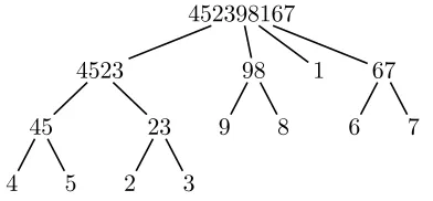
Figure 1.6:The substitution decomposition tree ofπ= 452398167.
mostly use.
Proposition 1.8(Albert and Atkinson [2]). Ifπis an inflation of12, then there is a unique sum
indecomposable α1 such that π = 12[α1, α2] for someα2, which is itself unique. The same holds
with12replaced by21and “sum” replaced by “skew”.
The substitution decomposition tree for a permutation then follows immediately. For example, consider the permutationπ= 452398167. This is decomposed as
452398167 = 2413[3412,21,1,12]
= 2413[21[12,12],21[1,1],1,12[1,1]]
= 2413[21[12[1,1],12[1,1]],21[1,1],1,12[1,1]]
CHAPTER
2
D
ECOMPOSITION
2.1 Background
S
INCE simple permutations may be used to construct all other permutations via thesubstitution decomposition, it would be useful to know how simple permutations are themselves constructed. In particular, our aim is to find smaller “fundamental” simple permutations of some specified size within a given simple permutation. Some approaches to this question can be found in Schmerl and Trotter [107], in which the following is proved for all irreflexive binary relational structures.1 Here, however, we will state only the
per-mutation case, for which there is another proof by Murphy [97].
Theorem 2.1(Schmerl and Trotter [107]). Every simple permutation of lengthn≥2contains a
simple permutation of lengthn−1orn−2.
We will prove that long simple permutations must contain two long almost disjoint simple subsequences. Formally:
Theorem 2.2. There is a functionf(k)such that every simple permutation of length at leastf(k)
contains two simple subsequences, each of length at leastk, sharing at most two entries.
(The proof of Theorem2.2follows after establishing Theorem2.14, found on Page34.) The second “two” in the statement of Theorem2.2is best possible, as is demonstrated by
1A version of this theorem fork-structures– structures defined on a singlek-ary relation in which every
relation(a1, . . . , ak)hasai=6 aj for somei6=j– can be found in Ehrenfeucht and McConnell [48].
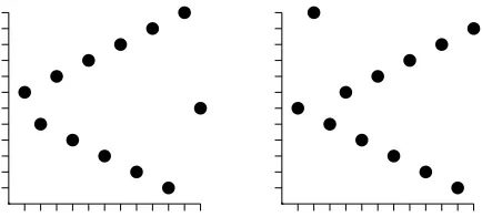
Figure 2.1:The plots of a wedge simple permutation. Note that every simple subsequence of length at least4must contain its first two entries.
the family of simple permutations of the form
m(2m)(m−1)(m+ 1)(m−2)(m+ 2)· · ·1(2m−1);
the permutation in Figure2.1is of this form. On the other hand, no attempt has been made to optimise the functionf; our proof gives anf of order aboutkk.
This result alone, however, gives no real indication as to the underlying structure within the simple permutation; rather it is the method by which we arrive at Theorem2.2. We give a Ramsey-type description of simple permutations in terms of some unavoidable substructures, similar to the Erd˝os-Szekeres Theorem as applied to arbitrary permutations:
Theorem 2.3 (Erd˝os and Szekeres [53]). Every permutation of length ncontains a monotone increasing or monotone decreasing subsequence of length at least √n.
In particular, we will demonstrate how a sufficiently long simple permutation contains, in the first instance, a “parallel alternation” of lengthk, a “wedge alternation” of lengthk
or a “pin sequence” of lengthk. By studying the decomposition of pin sequences, we can
go further to provide a more straightforward result, namely every sufficiently long simple permutation contains either an “alternation” or an “oscillation”.
2.2 PINSEQUENCES 23
p1
p2
p3 p1
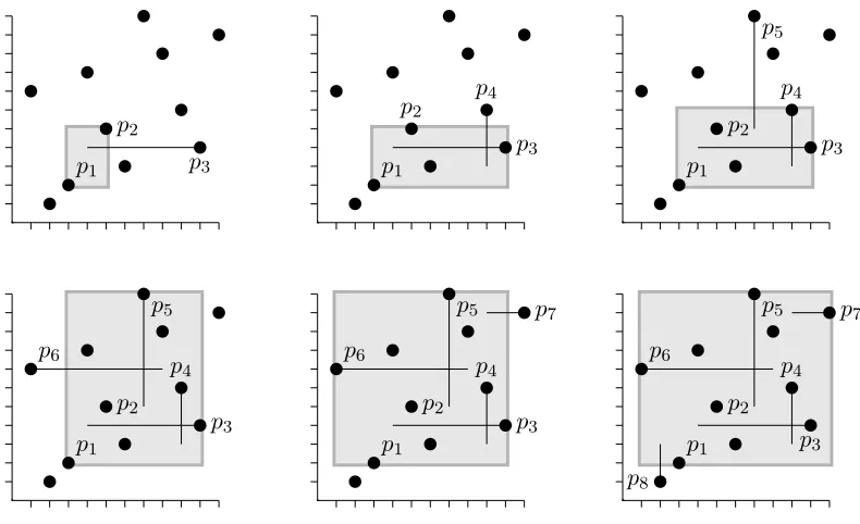
[image:40.612.92.487.48.289.2]p2 p3 p4 p1 p2 p3 p4 p5 p1 p2 p3 p4 p5 p6 p1 p2 p3 p4 p5 p6 p7 p1 p2 p3 p4 p5 p6 p7 p8
Figure 2.2:A pin sequence.
2.2 Pin Sequences
The core of the simple permutation decomposition is in understanding pin sequences. Em-pirically, they encapsulate precisely what it means to be simple: in the plot of a simple permutation, any set of points enclosed by an axis-parallel rectangle must be separated by at least one point lying outside the box above, below, to the left or to the right, and formalising the method of finding such a point is the motivation for defining pins, and subsequently sequences of pins.
While the viewpoint above will regard pins in their motivational setting as points
withinthe plot of a permutation, when we come to discussing our final “unavoidable sub-structures” result, we are going to need to decompose these pin sequences. To do this, we will shift our viewpoint to building pin sequences from scratch by placing points in a plane, each of which will correspond to a pin. We will also need to consider subsequences of a given pin sequence, for which we will need to introduce “pin words”.
in our original setting. Recall the graphical representation of a permutation as described in Section1.2. Given pointsp1, . . . , pmin the plane, we denote byrect(p1, . . . , pm)the smallest
axes-parallel rectangle containing them.
Choose two pointsp1 andp2 in the plot of a permutation π. If these two points do not form an interval then there is at least one point which lies outside rect(p1, p2) and slicesrect(p1, p2)either horizontally or vertically. (This discussion is accompanied by the sequence of diagrams shown in Figure 2.2.) We call such a point a pin. Choose a pin and label it p3. Now consider the larger rectangle rect(p1, p2, p3). If this also does not form an interval inπ then we can find another pin,p4, which slicesrect(p1, p2, p3) either horizontally or vertically. Again, if rect(p1, p2, p3, p4) is not an interval then we can find another pinp5. We refer to a sequence of pins constructed in this manner as apin sequence. Formally, a pin sequence is a sequence of pointsp1,p2,. . . in the plot ofπsuch that for eachi≥3,
• pi6∈rect(p1, . . . , pi−1), and
• ifrect(p1, . . . , pi−1) = [a, b]×[c, d]andpi = (x, y), we have eithera < x < borc < y < d, or, in other words,pi slicesrect(p1, . . . , pi−1)either horizontally or vertically. We describe pins as either left, right, up, or down based on their position relative to the rectangle that they slice. Thus in the pin sequence from Figure2.2,p3andp7are right pins,
p4andp5are up pins,p6is a left pin, andp8is a down pin (p1andp2lack direction). Aproper pin sequenceis one that satisfies two additional conditions:
• Maximality condition: each pin must be maximal in its direction. For example, if
rect(p1, . . . , pi−1) = [a, b]×[c, d]andpi = (x, y)is a right pin, then it is the right-most
of all possible right pins for this rectangle, or, in other words, the region(x, n]×[c, d] is devoid of points.
2.2 PINSEQUENCES 25
rect(p1, . . . , pi−2)
pi−1
pi pi+1
rect(p1, . . . , pi−2)
pi−1
pi
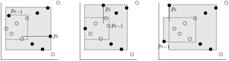
[image:42.612.103.478.56.163.2]pi+1
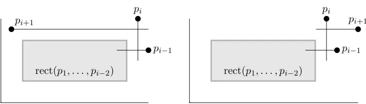
Figure 2.3:The two cases in the proof of Lemma2.6.
For example, in the pin sequence shown in Figure 2.2, the choice ofp4 violates the maxi-mality condition, while the choices ofp5,p7, andp8violate the separation condition. The ultimate goal of the following succession of lemmas is to show (in Theorem 2.7) that all or all but one of the pins in a proper pin sequence themselves form a simple permutation. We begin by observing that proper pin sequences travel by90◦ turns only.
Lemma 2.4. In a proper pin sequence,pi+1 cannot lie in the same or opposite direction aspi (for alli≥3).
Proof. By the maximality condition,pi+1cannot lie in the same direction aspi. It cannot lie
in the opposite direction by the separation condition.
Lemma 2.5. In a proper pin sequence,pidoes not separate any two members of{p1, . . . , pi−2}.
Proof. Ifpidid separaterect(p1, . . . , pi−2)into two parts thenpi−1 would lie on one side of this divide, violating the separation condition.
Lemma 2.6. In a proper pin sequence, pi and pi+1 are separated either by pi−1 or by each of
p1, . . . , pi−2.
We are now ready to prove our main result about proper pin sequences.
Theorem 2.7. If p1, . . . , pm is a proper pin sequence of length m ≥ 5 then one of the sets of points{p1, . . . , pm},{p1, . . . , pm} \ {p1}, or{p1, . . . , pm} \ {p2}is order isomorphic to a simple
permutation.
Proof. We are interested in the possible intervals in the subsequence given by the pins
p1, . . . , pm; we shall call theseintervals of pins. The bulk of our proof is devoted to
establish-ing the followestablish-ing claim: for any m, the only possible proper minimal nonsingleton
inter-vals of pins in the proper pin sequence{p1, . . . , pm}are{p1, pm},{p2, pm},{p1, p3, . . . , pm}
or{p2, . . . , pm}.
TakeM ⊆ {p1, . . . , pm}to be a minimal non-singleton interval of pins. Note thatM is
therefore order isomorphic to a simple permutation. IfM contains a pair of pinspi andpj
withi < j < mthen by the separation conditionpj+1, . . . , pm∈M. Furthermore, because j < m, Lemma2.6shows thatM contains eitherpj−1orp1, p2, . . . , pj−2. In the latter case, ifj≥4then separation givespj−1 ∈M, as desired, while ifj≤3, we have already found a minimal non-singleton interval of pins of the desired form. In the former case, the proof is completed by iterating this process. Only the caseM ={pi, pm}remains. If3≤i≤m−1
then by the separation conditionpiseparates{p1, . . . , pi−1}, while Lemma2.5shows that
pmdoes not separate these points; thus at least one of them must lie inM, a contradiction
which completes the proof of the claim.
Returning to the proof of the theorem, suppose that {p1, . . . , pm} is not itself order
isomorphic to a simple permutation and thatm ≥ 5. Thus, by the claim, at least one of
{p1, pm}, {p2, pm},{p1, p3, . . . , pm}or{p2, . . . , pm}forms a minimal nonsingleton interval
of pins. The latter two cases give us a simple of the desired form, so now assume either
{p1, pm}or{p2, pm}is an interval of pins. (Note that we cannot have both intervals since p3separatesp1fromp2.) We assume the former as the latter is analogous. Consider the pin sequence {p2, . . . , pm}. By the claim, the only possible minimal nonsingleton intervals of
pins in this sequence are{p2, pm},{p3, pm},{p2, p4, . . . , pm}or{p3, . . . , pm}. The latter two
2.2 PINSEQUENCES 27
was{p1, pm}, and hence the points thatp1 separated are the same as those separated by
pm. Thus it remains to eliminate the cases {p2, pm} and {p3, pm}. Since p3 separatesp1 fromp2 and{p1, pm}is an interval,p3also separatesp2 frompm, so{p2, pm}cannot form
an interval of pins for the sequence{p2, . . . , pm}. Similarly,{p3, pm}cannot be an interval
of pins for{p2, . . . , pm}becausep4separatesp3fromp1and thus also frompmbecause we
have assumed that{p1, pm} forms an interval. Thus{p2, . . . , pm} contains no nontrivial
intervals of pins and is therefore order isomorphic to a simple permutation, completing the proof.
As a corollary of this theorem, we see that Theorem2.2(in fact, a stronger result) is true for simple permutations with long pin sequences.
Corollary 2.8. Ifπcontains a proper pin sequence of length at least 2k+ 2(withk ≥4) thenπ contains two disjoint simple subsequences, each of length at leastk.
Proof. Apply Theorem2.7to the two pin sequencesp1, . . . , pk+1andpk+2, . . . , p2k+2.
We say that the pin sequencep1, . . . , pmfor the permutationπof lengthnissaturatedif rect(p1, . . . , pm) = [n]×[n]. For example, the pin sequence in Figure2.2is saturated. Any
two pointsp1 6=p2in the plot of a simple permutation can be extended to a saturated pin sequence, as we are forced to stop extending a pin sequence only upon finding an interval or when the rectangle contains every point inπ.
It is important to note that two points in a simple permutation need not be extendable to a proper saturated pin sequence. For example, the permutation in Figure 2.2does not have a proper saturated pin sequence beginning withp1 andp2. For this reason we work with a weaker requirement: the pin sequencep1, . . . , pm is said to beright-reachingifpm is
the right-most point ofπ.
Lemma 2.9. For every simple permutationπ and pair of pointsp1 andp2 (unless, trivially,p1is
Figure 2.4:A horizontal alternation (left) and its inverse, a vertical alternation (right).
Proof. Clearly we can find a saturated pin sequencep1, p2, . . . inπthat satisfies the maxi-mality condition. Since this pin sequence is saturated, it includes the right-most point; la-bel itpi1. Now takei2as small as possible so thatp1, p2, . . . , pi2, pi1 is a valid pin sequence.
Note first that i2 < i1 because p1, . . . , pi1 is a valid pin sequence. Now observe thatpi1
separatespi2 fromrect(p1, . . . , pi2−1), becausep1, . . . , pi2−1, pi1 is not a valid pin sequence.
Continuing in this manner, we find pinspi3,pi4, and so on, until we reach the stage where pim+1 =p2. Thenp1, p2, pim, pim−1, . . . , pi1 is a proper right-reaching pin sequence.
2.3 Simple Permutations without Long Proper Pin Sequences
It remains only to consider those simple permutations without long proper pin sequences. Lemma 2.9 shows that in such a permutation, any two points p1, p2 can be extended to a short proper right-reaching pin sequence. Our goal in this section is to use several of these short right-reaching sequences to prove that such permutations contain long “alter-nations”.
2.3 SIMPLEPERMUTATIONS WITHOUTLONG PROPERPINSEQUENCES 29
Figure 2.5:The two permutations on the left are wedge alternations, the two on the right are parallel alternations.
Proposition 2.10. Every alternation of length at least 2k4 contains either a parallel or wedge alternation of length at least2k.
Proof. Let π be a vertical alternation of length 2n ≥ 2k4. By the Erd˝os-Szekeres
Theo-rem2.3, the sequenceπ(1), π(3), . . . , π(2n−1)contains a monotone subsequence of length at leastk2, sayπ(i1), π(i2), . . . , π(ik2). Applying the Erd˝os-Szekeres Theorem to the
subse-quenceπ(i1+ 1), π(i2+ 1), . . . , π(ik2 + 1)completes the proof.
Note that every parallel alternation of length2k+ 2≥10contains two disjoint simple permutations of length at leastk. Thus Theorem2.2follows in the case where our simple
permutation contains a long parallel alternation.
Returning to pin sequences, the pin sequencesp1, p2, . . . andq1, q2, . . . are said to
• beinitially-nonoverlappingifrect(p1, p2)andrect(q1, q2)are disjoint,
• converge at the pointxif there existiandjsuch thatpi=qj =xbut{p1, . . . , pi−1}and
{q1, . . . , qj−1}are disjoint.
A collection of pin sequences converges or is initially-nonoverlapping if they pairwise converge or are pairwise initially-nonoverlapping. Note that it is always possible to find a collection ofbn/2cinitially-nonoverlapping proper pin sequences in a permutationπ of
length nby taking proper pin sequences beginning with the first and second points, the
third and fourth points, and so on, reading left to right.
Proof. Suppose that 16k initially-nonoverlapping proper pin sequences converge at the
pointx. Note thatxcan be the first or second pin for at most one of these sequences because
they are initially-nonoverlapping. Thus one of the following two possibilities must occur:
• at least8kof the sequences havexas their third pin, or
• at least8kof the sequences havexas their fourth or later pin.
Suppose that at least8k of the sequences havexas their third pin. This point could be
variously functioning as a left, right, down, or up pin for each of these8k sequences, but x plays the same role for at least2k sequences. Suppose, by symmetry, that xis a right
pin for at least2k sequences. Sincexis the third pin for these sequences, one of their first
two pins lies abovexwhile the other lies below and because these sequences are
initially-nonoverlapping, an alternation of length at least2kcan be obtained by choosing one point
from each sequence.
Now suppose that at least8kof the sequences havexas their fourth or later pin. Again
we may assume without loss thatx is a right pin for at least2kof these sequences. Now
consider the immediate predecessors to x in these sequences. These pins are either up
pins or down pins (by Lemma 2.4). By symmetry we may assume that for at least k of
these sequences the immediate predecessor toxis an up pin. Reading left to right, label
these immediate predecessor pins p(1), p(2), . . . , p(k) and letR(i) denote the rectangle for
whichp(i)is a pin. Note that eachR(i)lies completely belowx, as otherwise the separation condition would preventxfrom followingp(i)in the corresponding pin sequence. We now
have the situation depicted in Figure2.6.
It suffices to show, for eachi, thatπcontains a point lying horizontally betweenp(i)and
p(i+1)and belowxsince these points, together with thep(i)’s andx, will give an alternation
of length 2k. However, if there is no such point thenp(i) andp(i+1) could each function as up pins for both R(i) andR(i+1), and thus one of these choices would contradict the
2.3 SIMPLEPERMUTATIONS WITHOUTLONG PROPERPINSEQUENCES 31
R(1)
R(2) R(3)
R(4)
x p(1)
p(2)
[image:48.612.200.382.55.232.2]p(3) p(4)
Figure 2.6:The situation that arises in the proof of Lemma2.11.
Lemma 2.12. Every simple permutation of length at least2(16k4)2kcontains either a proper pin
sequence of length at least2kor a parallel or wedge alternation of length at least2k.
Proof. Suppose that a simple permutationπ of lengthncontains neither a proper pin
se-quence of length at least2k nor a parallel or wedge alternation of length at least 2k. In
particular, π does not contain a proper right-reaching pin sequence of length 2k, and it
follows from Proposition2.10thatπhas no alternations of length2k4.
It follows from our earlier observations thatπcontains a collection ofbn/2c
initially-nonoverlapping proper right-reaching pin sequences. As these sequences are right-reach-ing, they all have the same final (right-most) pin which we denote by p. By Lemma 2.11,
fewer than 16k4 of these pin sequences converge atp; equivalently, there are fewer than
16k4distinct immediate predecessors top, and we label these asp(1), p(2), . . . , p(m). Again,
fewer than16k4pin sequences converge at each of thep(i)’s, so there are fewer than(16k4)2 immediate predecessors to these pins. Continue this process until we reach the sequences of length2k, of which we have assumed there are none. We have thus counted allbn/2cof our sequences, and have obtained the bound
Figure 2.7:The two types of wedge simple permutations, type1(left) and type2(right).
so, simplifying,
n <2(16k4)2k.
We are left to deal with simple permutations which do not have long proper pin se-quences but do have long wedge alternations. We prove that these permutations contain longwedge simple permutations, of which there are two types (up to symmetry). Examples of these two types are shown in Figure2.7.
Lemma 2.13. If a simple permutation contains a wedge alternation of length4k2 then it contains either a pin sequence of length at least2kor a wedge simple permutation of length at least2k.
Proof. Let π be a simple permutation containing a wedge alternation of length at least
4k2. By symmetry we may assume that this wedge alternation opens to the right (i.e.
it is oriented as <). We call these thewedge points of π. Label the two left-most wedge
pointsp1andp2and by Lemma2.9extend this into a proper right-reaching pin sequence
p1, p2, . . . , pm.
LetRidenote the smallest rectangle in the plot ofπcontainingp1,p2, andpithat is not
sliced by a wedge point outside the rectangle. Define thewedge sumof the pinpi,ws(pi),
to be the number of wedge points in Ri. Fori ≥ 2define thewedge contribution ofpi by wc(pi) = ws(pi)−ws(pi−1)and setwc(p1) = 1. Regarding these quantities we make four observations:
(W1) the wedge sum of pm is equal to the total number of wedge points and also to m
X
i=1
2.3 SIMPLEPERMUTATIONS WITHOUTLONG PROPERPINSEQUENCES 33
pi−1
pi
pi−1
pi
pi−1
[image:50.612.100.482.49.151.2]pi
Figure 2.8:The three cases in the proof of Lemma2.13; the solid points form simple permutations.
(W2) it is not hard to construct examples in which pins have negative wedge contribu-tions; indeed,
(W3) left pins cannot have positive wedge contributions, and finally,
(W4) ifpiis an up pin, then the right-most wedge point inRiis an upper wedge point.
We now claim that eachpilies in a wedge simple permutation of length at leastwc(pi)+ 2. This claim implies the theorem, because if no pin lies in a wedge simple permutation of length at least2kthenwc(pi)≤2k−3, so by (W1),
4k2 ≤
m X
i=1
wc(pi)≤m(2k−3),
and thusm≥2k, giving the long pin sequence desired.
The claim is easily observed fori = 1 and, by (W3), vacuously true ifpi is a left pin.
Thus by symmetry there are only three cases to consider: an up pin followed by a right pin, a right pin followed by an up pin, and a left pin followed by an up pin. These three cases are depicted in Figure2.8.
Let us consider in detail the case of an up pin followed by a right pin. By (W4), the left-most wedge point inRi\Ri−1lies belowp1. By separation,pi−1lies abovepi, which is
itself the right-most point inRi. Therefore the wedge points inRi\Ri−1together withpi
wedge simple permutation of type2, while in the left-up case a wedge simple permutation of type2can be formed from the wedge points inRi\Ri−1,pi−1, andpi.
We have therefore established the following theorem.
Theorem 2.14. Every simple permutation of length at least 2(256k8)2k contains a proper pin
sequence of length2k, a parallel alternation of length2k, or a wedge simple permutation of length
2k.
The proof of Theorem 2.2 now follows by analysing each of these cases in turn. A parallel alternation of length 2k + 2 ≥ 10 contains two disjoint simple permutations of length k. A type1 wedge simple permutation of length 2k contains two type 1 wedge simple permutations of length k with only one entry in common, and a type 2 wedge simple permutation of length2kcontains two type2wedge simple permutations of length
k which share two entries. Finally, Corollary 2.8shows that a permutation with a proper
pin sequence of length2k+ 2contains two disjoint simple permutations of lengthk.
2.4 Pin Words
To explain how to expatiate Theorem2.14into a simpler “unavoidable substructures” re-sult, we must first change our viewpoint so we can consider arbitrary proper pin sequences and their subsets, rather than pin sequences within a given simple permutation. This treat-ment will also be of use in Part II. To this end we extend the pin sequence definition to allow us to place points in the plane as they are required. While the precise coordinates of each pin will be far from unique, we do not encounter any difficulties as two sets of points in the plane constructed by the same pin sequence will be order isomorphic.
The changing viewpoint requires that we replace the maximality condition with the “externality” condition. Formally, aproper pin sequenceis a sequence of points in the plane satisfying: