Development and application of a global magnetic field evolution model for the solar corona

(1)

DEVELOPMENT AND APPLICATION OF A GLOBAL FIELD

EVOLUTION MODEL FOR THE SOLAR CORONA

Anthony Robinson Yeates

A Thesis Submitted for the Degree of PhD

at the

University of St. Andrews

2009

Full metadata for this item is available in the St Andrews

Digital Research Repository

at:

https://research-repository.st-andrews.ac.uk/

Please use this identifier to cite or link to this item:

http://hdl.handle.net/10023/734

This item is protected by original copyright

(2)

DEVELOPMENT AND

APPLICATION

OF A

G

LOBAL

M

AGNETIC

F

IELD

E

VOLUTION

M

ODEL FOR

THE

S

OLAR

CORONA

Anthony Robinson Yeates

Thesis submitted for the degree of Doctor of Philosophy

of the University of St Andrews

(3)

(4)

Abstract

Magnetic fields are fundamental to the structure and dynamics of the Sun’s corona. Obser-vations show them to be locally complex, with highly sheared and twisted fields visible in solar filaments/prominences. The free magnetic energy contained in such fields is the primary source of energy for coronal mass ejections, which are important—but still poorly understood—drivers of space weather in the near-Earth environment.

In this thesis, a new model is developed for the evolution of the large-scale magnetic field in the global solar corona. The model is based on observations of the radial magnetic field on the solar photosphere (visible surface). New active regions emerge, and their transport and dispersal by surface motions are simulated accurately with a surface flux transport model. The 3D coronal magnetic field is evolved in response to these photospheric motions using a magneto-frictional technique. The resulting sequence of nonlinear force-free equilibria traces the build-up of mag-netic helicity and free energy over many months.

The global model is applied to study two phenomena: filaments and coronal mass ejections. The magnetic field directions in a large sample of observed filaments are compared with a 6-month simulation. Depending on the twist of newly-emerging active regions, the correct chirality is simulated for up to 96% of filaments tested. On the basis of these simulations, an explanation for the observed hemispheric pattern of filament chirality is put forward, including why exceptions occur for filaments in certain locations. Twisted magnetic flux ropes develop in the simulations, often losing equilibrium and lifting off, removing helicity. The physical basis for such losses of equilibrium is demonstrated through 2D analytical models. In the 3D global simulations, the twist of emerging regions is a key parameter controlling the number of lift-offs, which may explain around a third of observed coronal mass ejections.

(5)

(6)

v

Declaration

I, Anthony Yeates, hereby certify that this thesis, which is approximately 55,000 words in length, has been written by me, that it is the record of work carried out by me and that it has not been

submitted in any previous application for a higher degree.

Candidate:Anthony Yeates Signature: ... Date: ...

I was admitted as a research student in October 2005 and as a candidate for the degree of Doctor

of Philosophy in October 2006; the higher study of which this is a record was carried out in the

University of St Andrews between 2005 and 2008.

I hereby certify that the candidate has fulfilled the conditions of the Resolution and Regulations

appropriate for the degree of Doctor of Philosophy in the University of St Andrews and that the candidate is qualified to submit this thesis in application for that degree.

Supervisor:Duncan Mackay Signature: ... Date:

Supervisor:Eric Priest Signature: ... Date: ...

In submitting this thesis to the University of St Andrews I understand that I am giving permission

for it to be made available for use in accordance with the regulations of the University Library for

the time being in force, subject to any copyright vested in the work not being affected thereby . I also understand that the title and abstract will be published, and that a copy of the work may be

made and supplied to any bona fide library or research worker, that my thesis will be electronically

accessible for personal or research use, and that the library has the right to migrate my thesis into new electronic forms as required to ensure continued access to the thesis . I have obtained any

third-party copyright permissions that may be required in order to allow such access and migration .

The following is an agreed request by candidate and supervisor regarding the electronic publication of this

thesis:

Access to Printed copy and electronic publication of thesis through the University of St Andrews.

(7)

(8)

Acknowledgements

First and foremost, I would like to thank my supervisor Duncan Mackay for his ceaseless encour-agement and support. This work would not have been possible without him, nor without financial support from the UK Science and Technology Facilities Council (STFC). I have also been given much useful advice by Eric Priest, Thomas Neukirch, and all of the Solar and Magnetospheric Theory Group at St Andrews. My fellow PhD students in particular deserve much credit for or-ganising social activities, and for making my time here a happy one. I also thank Peter Jupp in the maths department for very useful advice on statistical tests.

Outside St Andrews, I must thank Aad van Ballegooijen for developing the original technique, for many suggestions, and for careful readings of my papers. I very much enjoyed two summers at the Solar Physics group at Montana State University; in particular I thank Dibyendu Nandy and Piet Martens (for funding my first visit and for an interesting and productive collaboration on dynamo theory), and Dick Canfield (for organising such an excellent REU programme). I am indebted to Sara Martin and the PROM group for supporting my visit to the 2006 PROM meeting in Virginia, and in particular to Art Poland for his kind hospitality. I thank also Jun Lin for suggestions on extending some of his work (developed in Chapter6of this thesis).

My time in St Andrews has been much enlivened by everyone in the Breakaway (St Andrews University Hill Walking) club, and by the staff and students of Deans Court. Last, but by no means least, I could not have got this far without the support of my parents and my fianc´ee Celia.

(9)

(10)

Publications

The following published papers include material from this thesis:

1. Yeates, A.R., Mackay, D.H., & van Ballegooijen, A.A.: 2007, ’Modelling the Global Solar Corona: Filament Chirality Observations and Surface Simulations’, Sol. Phys. 245, 87. 2. Yeates, A.R., Nandy, D., & Mackay, D.H.: 2008, ’Exploring the Physical Basis of Solar

Cycle Predictions: Flux Transport Dynamics and Persistence of Memory in Advection versus Diffusion Dominated Solar Convection Zones’, ApJ 673, 544.

3. Yeates, A.R., Mackay, D.H., & van Ballegooijen, A.A.: 2008, ’Modelling the Global Solar Corona II: Coronal Evolution and Filament Chirality Comparison’, Sol. Phys. 247, 103. 4. Mackay, D.H., Gaizauskas, V., & Yeates, A.R.: 2008, ’Where do Solar Filaments Form?

Consequences for Theoretical Models’, Sol. Phys. 248, 51.

5. Yeates, A.R., Mackay, D.H., & van Ballegooijen, A.A.: 2008, ’Evolution and Distribution of Current Helicity in Full-Sun Simulations’, ApJ 680, L165.

6. Yeates, A.R. & Mackay, D.H.: 2009, ’Modelling the Global Solar Corona III: Origin of the Hemispheric Pattern of Filaments’, Sol. Phys. 254, 77.

(11)

(12)

It will be found to be another and instructive instance of the regular irregularity and the irregular regularity which, in the present state of

our knowledge, appear to characterise the solar phenomena.

(R. C. Carrington: 1858, MNRAS 19, 1.)

(13)

(14)

List of Figures

1.1 Artist’s impression of the Sun. . . 2

1.2 Observations of the Sun’s magnetic field. . . 4

1.3 The solar magnetic activity cycle. . . 5

1.4 Twisted magnetic fields. . . 9

1.5 Filaments and coronal mass ejections. . . 10

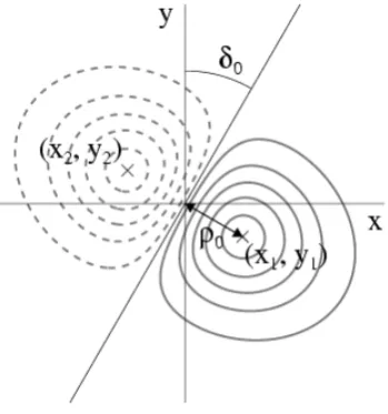
2.1 A tilted bipole. . . 19

2.2 Analytical solution at a sequence of times for bipole. . . 21

2.3 Sketch illustrating regions of integration. . . 26

2.4 Total magnetic fluxΦ(t)over time. . . 27

2.5 Comparison of numerical and analytical solutions. . . 30

2.6 Performance of Euler and mid-point schemes. . . 30

3.1 Large-scale surface flow profiles. . . 33

3.2 Transformation to computational coordinates. . . 34

3.3 Location of variables and indices on a grid cell. . . 35

3.4 Effect of diffusion on numerical stability. . . 36

3.5 Effect of initial bipole tilt angle in producing a polar field. . . 37

3.6 Correction of synoptic magnetograms for differential rotation. . . 39

3.7 Comparison between simulation with no emerging flux and observed magnetograms. 41 3.8 Stages in the processing of synoptic magnetograms for the detection of new bi-polar regions. . . 44

3.9 The semi-automated procedure to detect new flux regions. . . 44

3.10 Summary of properties of the 119 bipolar regions. . . 47

3.11 Results on day 147 for different methods of bipole insertion. . . 50

3.12 Comparison between observed magnetograms and simulation results using the two emerging flux techniques. . . 51

(21)

List of Figures xx

3.13 Use of flux transport simulations to determine filament source regions. . . 54

3.14 Number of filaments in each category as a function of phase of the solar cycle. . . 55

4.1 Cartoon of the coronal magnetic field evolution. . . 58

4.2 Potential field extrapolation for 1999 April 16. . . 64

4.3 A magnetic bipole. . . 65

4.4 Effect of the twist parameterβon a bipolar region. . . 66

4.5 Components of the sweeping procedure. . . 67

4.6 Example of bipole insertion process. . . 69

4.7 Snapshots of the global simulation run A4. . . . 71

4.8 Global magnetic field properties over the 177-day simulations. . . 72

4.9 Observations of current helicity against latitude. . . 75

4.10 Distribution of current helicity in and around a single bipolar region. . . 75

4.11 Global distribution ofα. . . 77

4.12 Height distribution ofαin a latitudinal plane. . . 78

4.13 Global distribution ofαfor different signs of inserted bipole twist. . . 79

5.1 Filaments with dextral and sinistral chirality. . . 83

5.2 Observations of the hemispheric pattern. . . 84

5.3 Formation of helical fields by flux cancellation and reconnection. . . 86

5.4 The head-to-tail linkage model. . . 87

5.5 Magnetic field structure for two bipoles interacting in the northern hemisphere. . 88

5.6 Example Hαobservations from BBSO. . . 90

5.7 Chirality of the 255 observed filaments on a time-latitude plot. . . 91

5.8 Observed filament locations overlayed on Kitt Peak synoptic magnetograms. . . . 92

5.9 Simulated coronal field structure at the location of observed filament 544. . . 93

5.10 Skew of the coronal magnetic field above a photospheric PIL. . . 93

5.11 Simulated skew along all photospheric PILs in run A4. . . . 94

5.12 Simulated skew at observed filament locations during CR1952. . . 95

5.13 Results of the chirality comparison. . . 97

5.14 Mechanisms which always produce the same type of skew. . . 100

5.15 Mechanisms which can produce either dextral or sinistral skew depending on in-dividual circumstances. . . 101

5.16 Simulated skew for filament 448, on the north polar crown. . . 103

5.17 Tilt angle of field lines across a polar crown PIL. . . 104

(22)

List of Figures xxi

5.19 Difference between simulated and expected field line tilt in 2.5D test simulations. 106 5.20 Simulated skew at the location of internal filaments 188 and 280b. . . 107 5.21 Shape of the field lines around the PIL of a bipole in a background field. . . 108 5.22 Example filament on the external PIL of a bipole. . . 109 5.23 Example where bipole emergence in a complex background field creates the

op-posite sign of skew. . . 110 5.24 Development of skew at location of filament 341. . . 111

6.1 Basic set-up of the quadrupolar point source model. . . 123 6.2 Bifurcation diagram in(λ, h)space for quadrupolar point source model, and

ex-amples of the 5 topologies. . . 125 6.3 Equilibrium curve and vertical force profile for the quadrupolar point source model.129 6.4 Evolution ofBy(x, t)on the solar surface, for the initial condition of a single bipole.134

6.5 TheBzandBθcomponents of the Gold-Hoyle solution. . . 137

6.6 The single bipole solution. . . 141 6.7 Time until loss of equilibrium, as a function of different parameters in the single

bipole model. . . 142 6.8 The quadrupolar solution. . . 144 6.9 The two phases of the quadrupolar boundary condition. . . 145

7.1 Formation and lift-off of an example flux rope. . . 150 7.2 Magnetic field structure of the flux rope shown in Figure7.1. . . 151 7.3 Automatic detection of flux rope “points” and clustering into separate ropes. . . . 153 7.4 The time correlation procedure in action for a 2-day correlation period. . . 155 7.5 Flux ropes determined by the three-stage automated procedure over the 13-day

correlation period. . . 156 7.6 Examples of complex flux rope structures during the 13-day test period. . . 157 7.7 Flux rope statistics calculated on each day independently over the 177-day

(23)

List of Figures xxii

B.1 The domainV. . . 181

C.1 Schematic illustration of the time correlation procedure. . . 187

D.1 Meridional circulation and diffusion profiles in our model. . . 195 D.2 Two example solutions. . . 196 D.3 Dependence of cycle duration and cycle amplitude on the meridional circulation

speed. . . 198 D.4 Dependence of cycle amplitude on the poloidal diffusivity. . . 198 D.5 Transition between the advection-dominated and diffusion-dominated regimes. . 201 D.6 Comparison of poloidal fields in advection-dominated and diffusion-dominated

regimes. . . 202 D.7 Comparison of toroidal field in advection-dominated and diffusion-dominated

(24)

List of Tables

4.1 Summary of simulation runs analysed in this thesis. . . 70

5.1 Number of filament locations with each skew type, in each simulation run. For each type the table gives the number in the northern hemisphere / number in the southern hemisphere. The right column gives the percentage of locations which match the observed chirality. . . 96 5.2 Classification of filaments with wrongly simulated chirality, for each simulation run. 98 5.3 Classification of filaments by skew mechanism (as defined in Figures5.14 and

5.15). Simulation results presented here are for run A4. . . 113

7.1 Criteria used for detection of flux rope lift-offs. . . 162 7.2 Comparison of criteria for detecting flux rope lift-offs. . . 163 7.3 Number of flux rope lift-offs in each 177-day simulation run. . . 165

D.1 Cycle-to-cycle correlations for 275 cycles. . . 207

(25)

(26)

Chapter 1

Introduction

1.1 The Sun: Structure and Rotation

The Sun is a giant self-gravitating ball of plasma. It has a mass1.99×1030kg contained in a radiusR= 6.96×108m, and is over 90% hydrogen, with about 8% helium. The basic structure of the Sun and its atmosphere is illustrated in Figure 1.1, where it is seen to be divided into a number of layers.

The easiest layer to observe is the photosphere, or visible surface. The photosphere emits most of the Sun’s radiation into space, and is relatively dense and opaque. Since ancient times, dark sunspots have been observed at the photospheric level on the solar disk. Telescope observations of the Sun since about 1610 have followed both sunspots and also bright “faculae” near the limb, and since the 19th Century they have also revealed the mottled pattern of granulation (see below).

Figure1.1illustrates two outer layers of the Sun’s atmosphere: the chromosphere in red, and the

corona in blue/purple (false colour). For centuries these layers were visible only during solar

eclipses. The corona appeared as a white halo extending for severalR above the limb, and the chromosphere appeared for only a few seconds before and after totality, as a thin red annulus around the rim of the photosphere. More recently the chromosphere and corona have been imaged by a number of space-based telescopes in extreme ultra-violet and in soft X-rays. Surprisingly, the corona is very hot, at millions of kelvin, much hotter than the underlying photosphere which is around6,000K. This counter-intuitive property was first discovered in the late 1930s by Grotrian and Edl´en. Because the solar surface is cooler, the corona cannot be heated by thermal energy transport, so its heating must be nonthermal; theories suggest either waves or electric currents.

(27)

[image:27.595.59.484.121.464.2]

1.1 The Sun: Structure and Rotation 2

Figure 1.1: Artist’s impression illustrating the different layers of the Sun and its atmosphere. (Fromhttp://www.spaceweathercenter.org/resources/.)

observations, notably from helioseismology. The Sun has a huge power output of3.9×1023kW. It generates this energy by fusion of hydrogen into helium, and 99% of the energy is generated in the inner 20% of the Sun’s radius, called the core, at a temperature of the order1.5×107K. This energy is transmitted out from the core through the radiative zone, where photons are absorbed and re-radiated many times in a diffusion-like process, driven by establishing a temperature gradient. Above about0.7R, called the convection zone, the temperature gradient becomes too steep to maintain static equilibrium and convective instability sets in.

The upper-most convective cells are visible in images of the photosphere as the granulation pat-tern. The bright granules have typical size∼ 1 Mm, and are surrounded by dark inter-granular lanes. The pattern changes on a timescale of 5 minutes. A pattern of larger cells, called

super-granulation, is visible in Doppler images of the photospheric velocity. These cells are∼15 Mm

(28)

1.2 The Sun’s Magnetic Field 3

The earliest telescope observations of sunspots demonstrated that the Sun rotates, with a surface rotation speed of∼2 kms−1 near the equator. This is comparable with other stars of similar age and mass (whose rotation rates are known from modulation of emission lines as bright regions rotate across their disks;Soon, Frick, and Baliunas, 1999). It has long been known, since the sunspot observations of Scheiner in the 17th Century, that the solar surface rotates faster at the equator than at the poles. Viewed from Earth the rotation period is 26 days at the equator and about 36 days at the poles. This differential rotation pattern is steady to within 5%, and the profile inside the Sun has now been inferred from helioseismology down to about0.2R. The differential rotation is believed to be driven by the interaction of convection with the Sun’s overall rotation, the latter inducing anisotropic momentum and heat transport (Miesch, 2005). This interaction is also thought to drive the large-scale meridional circulation, which is an axisymmetric flow in the radius-latitude plane. This flow is much weaker than the differential rotation so is harder to measure (Hathaway,1996). However, there is a growing body of evidence for a poleward bulk surface flow of about10to20 ms−1. This is presumed to be counter-balanced by an equatorward flow low in the convection zone.

1.2 The Sun’s Magnetic Field

One of the key advances in solar physics was the discovery byHale(1908) that sunspots harbour extremely strong magnetic fields of up to3000 G. These measurements used the Zeeman splitting of spectral lines that occurs for atoms radiating in a strong magnetic field. In the 1950s, Babcock and Babcock used their newly-invented magnetograph to measure magnetic fields all over the solar disk (Babcock and Babcock, 1955). Figure1.2(a) shows a more recent full-disk magnetogram of the line-of-sight field taken by the MDI instrument on the SOHO satellite (Scherrer et al.,

1995).1 Although magnetic flux (shown by white and black regions) is distributed across the Sun, the highest concentrations are in bipolar active regions concentrated near the equator. These consist of neighbouring positive and negative polarities, usually oriented in an approximately east-west direction. These polarities often correspond to sunspots seen in white-light. Active regions represent concentrations of large-scale flux emergence, and also of activity such as solar flares. In ultra-violet or X-ray wavelengths, which are primarily emitted by coronal plasma, active regions show up brightly. This is seen in Figure1.2(b), which is an image from SOHO/EIT in the 195A filter (showing plasma at a temperature of˚ 1.6MK). In such images (notably those from the TRACE satellite, not illustrated here), the emission clearly outlines thin loops, which correspond to magnetic field lines because the plasma is constrained to follow the magnetic field. In surface magnetograms, such as Figure1.2, we are viewing the intersection of these field lines with the photosphere.

1

(29)

1.2 The Sun’s Magnetic Field 4

Figure 1.2: Observations of the Sun’s magnetic field. Panel (a) shows a full-disk line-of-sight magnetogram from SOHO/MDI on 2002 April 26. Panel (b) shows a co-temporal EUV image in the195A filter of SOHO/EIT. Panel (c) shows a recent magnetogram of a single bipolar region,˚ from the Solar Optical Telescope on Hinode (image produced by National Astronomical Observat-ory of Japan). In both magnetograms, white indicates positive field (i.e., toward the observer) and black indicates negative field. The Hinode magnetogram also measures the horizontal component of the magnetic field, shown by the red arrows.

Observations by Hale and colleagues demonstrated a number of fundamental laws governing the magnetic polarity of bipolar regions (Hale and Nicholson,1925). Firstly, all leading spots—i.e. in the direction of solar rotation—in the northern hemisphere have the same polarity (positive/white in Figure1.2a), and all leading spots in the southern hemisphere have the opposite polarity (neg-ative/black in the figure). Secondly, the leading spot tends to be closer to the equator than the following spot in each bipolar pair (Hale et al., 1919, known as Joy’s Law). Finally, all of the polarities reverse approximately every 11 years. The first and second laws may be seen in Figure 1.2(a).

In the weeks and months after they initially emerge, bipoles are observed to break up and spread; some resulting regions of weaker, diffuse magnetic flux may be seen surrounding the strong re-gions in Figure1.2. In the 1960s, R. Leighton explained how supergranule motions break up the magnetic field and spread the photospheric footpoints of field lines in a random walk, which he modelled by a diffusion process (Leighton,1964, see also Chapter2). He demonstrated how the field is concentrated into the thin “network” of boundaries between the supergranular cells. This magnetic network may be seen in Figure1.2(c), which is a recent (2006 December 12) magneto-gram of a single bipolar region from the Solar Optical Telescope (Tsuneta et al.,2008) on the Hinode satellite. Outside the main sunspots the field is seen to concentrate into discrete flux tubes (of kilogauss field strength), rather than to be distributed evenly over the solar surface.

(30)

me-1.3 Modelling the Coronal Magnetic Field 5

Figure 1.3: The solar magnetic activity cycle, shown by (a) a latitude-time plot of longitude-averaged radial magnetic field on the solar surface (David Hathaway, NASA), and (b) a plot of smoothed monthly International Sunspot Number since the year 1750. The sunspot data is from the SIDC-team, World Data Center for the Sunspot Index, Royal Observatory of Belgium (http: //www.sidc.be/sunspot-data/). In (a) yellow indicates positive magnetic field and blue negative, as given by the legend.

ridional circulation, leads to the cyclic reversal of the Sun’s polar fields—i.e. those above60◦ latitude—first measured byBabcock and Babcock(1955). While leading polarity flux tends to cancel across the equator, following polarity flux tends to be transported poleward by a combina-tion of diffusion and the meridional flow. This creates an excess of one polarity at high latitudes over each 11 year cycle, which eventually reverses the opposite-polarity polar field from the previ-ous cycle. Such reversals are visible in Figure1.3(a), which shows the longitude-averaged surface magnetic field on a time-latitude plot (yellow for positive flux, blue for negative). Also visible is the equatorward migration of sunspot emergence latitudes through each 11-year cycle. This reg-ular solar cycle is also evident in the number of sunspots over time, plotted since 1750 in Figure 1.3(b). This magnetic cycle modulates all forms of solar activity, and has its origin in a dynamo mechanism in the solar interior, which is still poorly understood.

1.3 Modelling the Coronal Magnetic Field

(31)

1.3 Modelling the Coronal Magnetic Field 6

On a macroscopic scale, the evolution of an electrically conducting fluid interacting with a mag-netic field is well-described by the equations of magnetohydrodynamics (MHD; e.g.Priest,1982). In MHD, the plasma—which in reality consists of a mixture of electrons and ions—is treated as a single fluid with bulk velocityv, pressurep, and densityρ, with a magnetic fieldB. The magnetic field is restricted by the solenoidal constraint,

∇ ·B= 0, (1.1)

which asserts that there are no magnetic monopoles. In MHD, Maxwell’s equations are simplified by assuming that all motions are much slower than the speed of light, so that the displacement current may be neglected. Then Amp`ere’s Law reads

∇ ×B=µj, (1.2)

whereµis the magnetic permeability (assumed constant) andjis the electric current density. The third Maxwell equation is Faraday’s Law

∇ ×E=−∂B

∂t . (1.3)

For the large spatial scales of interest in the solar corona, it is also valid to assume charge neut-rality, which means that the electric charge density may be neglected and thus so may be the fourth Maxwell equation (conservation of electric charge density). In order to close the system of electromagnetic equations, we also require Ohm’s Law,

j=σ(E+v×B), (1.4)

whereσ is the electrical conductivity (assumed constant). This is actually a simplified form of the full Ohm’s Law obtained by taking moments of kinetic equations. With these equations and assumptions the electric fieldEmay be eliminated entirely by combining (1.1), (1.2), (1.3), and (1.4) to give the so-called MHD induction equation

∂B

∂t =∇ ×(v×B) +η∇

2_B_, _(1.5)

whereη = 1/(µσ)is the magnetic diffusivity. The first term in (1.5) represents the advection of the magnetic field by plasma motions, while the second represents diffusion of the magnetic field. The physics of advection and diffusion are demonstrated in Chapter2.

In addition to the electromagnetic equations above, the MHD equations include the continuity, momentum, and energy equations as in ordinary fluid dynamics. The mass continuity equation takes its usual form

∂ρ

(32)

The magnetic field and plasma velocity are coupled both through Ohm’s Law (1.4) and through the Lorentz force term (j×B) in the momentum equation, which reads

ρDv

Dt =−∇p+j×B+ρg. (1.7)

Heregis the acceleration due to gravity, and we have neglected viscous terms. The energy equa-tion takes the form

ργ γ−1

D Dt

p ργ

=−L, (1.8)

whereγ is the ratio of specific heats andL is the total energy loss function, which in general includes terms due to thermal conduction, radiation, and ohmic heating.

The MHD description of a plasma is valid assuming that the plasma is sufficiently collisional, which essentially equates to MHD timescales being much longer than collision timescales. A fluid description also requires that the macroscopic lengthscale be much longer than the mean free path of particles, which is satisfied even in the corona where the mean free path is tens of kilometres.

1.3.1 Force-free Equilibria

In this thesis we do not solve the time-dependent MHD equations in the corona, but rather we con-sider equilibria. In the global corona, we may then simplify equation (1.7) concon-siderably. Firstly, velocity variations may be neglected since|v| vA, wherevA= |B|/

√

µρis the Alfv´en speed (approximately1000km s−1 in the corona). Secondly, we may neglect the gravity term as com-pared to the pressure gradient providing the lengthscale of interest is less than the pressure scale-height, which is typically of order105km in the corona. Finally, the pressure gradient may be neglected compared to the Lorentz force since, in the corona,β 1. The plasma β parameter is the ratio of gas pressure, p, to magnetic pressure, B2/(2µ). Thus the magnetic field in the solar corona—except during dynamic events such as coronal mass ejections—may be expected to satisfy

j×B= 0. (1.9)

Such a field is called force-free, since the Lorentz force vanishes everywhere.

1.3.2 Potential Fields

Equation (1.9) is, unfortunately, nonlinear and hence difficult to solve. A simple solution may be obtained by takingj= 0everywhere, which is called a potential field. In that case one may write

(33)

potential extrapolations from photospheric magnetograms to model the coronal magnetic field. The existence and uniqueness of a solutionψ is assured for suitable lower and upper boundary conditions. Numerical computations for the global corona tend to use the observed radial pho-tospheric magnetic field on the lower boundary, and a “source surface” whereB is forced to be radial on the upper boundary (after Altschuler and Newkirk,1969;Schatten, Wilcox, and Ness,

1969). In AppendixBwe prove uniqueness for the particular boundary conditions used for the 3D simulations in this thesis. When compared to EUV or X-ray images showing the coronal structure, these potential field extrapolations match reasonably well. Closed magnetic field lines correspond to areas with EUV or X-ray loops on the disk (visible in Figure1.2b), or bright streamers above the limb. Open field regions correspond to locations of “coronal holes” (dark in EUV; Figure 1.2b).

1.3.3 Free Energy: Nonlinear Force-free Fields

The weakness of the potential field model is that it has the minimum magnetic energy among all magnetic fields satisfying the same boundary conditions. This is proved in AppendixBfor the 3D domain and boundary conditions used in this thesis. The potential field has no free magnetic

energy available for conversion into heat or kinetic energy to power activity such as flares or

eruptions. A typical CME requires∼1032ergs of kinetic energy alone, and the magnetic field is the only possible source of such energy in the corona (Forbes,2000).

In general, equation (1.9) for a force-free field is satisfied if

j=αB, (1.10)

whereα(x)is a scalar function of position. Note that taking the divergence of (1.10) gives(B· ∇)α = 0, so thatα must be constant along magnetic field lines, although it may vary between different field lines. The value ofαdescribes the helical twist of a field line with respect to the potential fieldα = 0 (Sakurai,1979, Appendix 2), as illustrated in panels (a) and (b) of Figure 1.4. Panels (c) and (d) show observations by the Hinode X-ray Telescope2 of coronal loops in two active regions which exhibit the two signs of twist. These so-called “sigmoid” (S-shaped) patterns demonstrate the non-potential magnetic fields found in active regions, particularly those with flaring or eruptive activity.

Ifαis taken to be constant everywhere, then the magnetic field is called linear force-free. Equa-tion (1.10) is then linear and easily solved. However, for a force-free field,αis equal to the current helicity (a quantity discussed in Section4.7), and the current helicity is known to vary significantly

2

(34)

1.4 Motivation: Filaments and Eruptions 9

Figure 1.4: Twisted magnetic fields. Panels (a) and (b) show the direction of twist for a force-free field line with (a) positiveα, and (b) negative α, with respect to the potential field. Panels (c) and (d) show X-ray sigmoid structures with each sign of twist, observed in active regions with the Hinode X-ray Telescope (SAO, NASA, JAXA, NAOJ). These images were taken on 2007 February 16 and 2007 February 5 respectively.

over even quite small regions of the photosphere. Therefore linear force-free fields are not appro-priate for global coronal modelling and we do not consider them in this thesis. Instead, we allow

αto be a function of position and model nonlinear force-free fields; our technique is described in Chapter4.

1.4 Motivation: Filaments and Eruptions

Although potential magnetic fields are adequate for modelling the general structure of open and closed field regions in the corona, there are important phenomena which depend, for their ex-istence, on twisted and sheared nonpotential configurations. The aim of this thesis is to apply a nonlinear force-free evolution model to study two such phenomena: filaments and coronal mass ejections.

(35)

1.4 Motivation: Filaments and Eruptions 10

Figure 1.5: Filaments and coronal mass ejections. Panel (a) shows both filaments against the disk and a prominence above the limb, in Hα(image courtesy of J. Newton). Panel (b) shows a twisted erupting filament in the 304A line of SOHO/EIT (showing upper chromospheric temperatures˚ ∼60,000K). Panel (c) shows a typical 3-part CME in the LASCO/C3 coronagraph on SOHO.

at6563_{A, toward the red end of the visible spectrum. Filaments show up as thin, dark, absorp-}˚ tion structures against the solar disk (Figure1.5a). Above the limb they are visible in emission (also Figure1.5a), where they are traditionally known as prominences, although prominences and filaments are the same physical object.

Filaments/prominences are found over a wide range of latitudes, from the activity belts (0◦to30◦) to the polar crowns (c. 60◦). Observations have long recognised a variation in properties such as size, lifetime, stability, magnetic field, and temperature (Tandberg-Hanssen,1974). They are loosely labelled either “active” or “quiescent”, in a basic two-class classification that originates withSecchi(1875), who, incidentally, was the first to introduce both photographic and spectro-graphic methods into eclipse observations. Active prominences are dynamic, short-lived structures (lasting minutes to hours) located in active regions and often associated with flares. In contrast, quiescent prominences are long-lived, stable structures that may last for many months and grow to lengths of up to a solar radius. In this thesis we simulate the large-scale magnetic field in a sequence of equilibria, so are concerned with the quiescent type.

The magnetic field is vital for the existence of filaments because it supports the filament mass against gravity, via the Lorentz force. We describe observations of filament magnetic fields in Chapter5. Suffice it to say here that the magnetic field in a quiescent filament is approximately horizontal, and lies along the long axis of the filament, which itself always lies along a polarity inversion line in the photospheric field. Thus filament magnetic fields are highly sheared and cannot be modelled by potential fields. In addition, many quiescent filaments end their life by erupting, and in that case are often observed to be helically twisted (Figure1.5b).

(36)

1.5 Thesis Outline 11

from SOHO/LASCO3, show coronal density via Thompson scattering of photospheric light by coronal electrons. A time-sequence of another CME observed by LASCO is illustrated in Chapter 7, Figure7.11. A typical CME injects1016g of coronal material and1023Mxof magnetic flux into interplanetary space. The outward speed is often several hundred kilometres per second, requiring ∼ 1032ergs of energy to accelerate the mass against gravity. We have already indicated above that this amount of energy can only come from the magnetic field. When directed Earthward, CMEs (and the associated energetic particles) are the primary cause of space weather hazards in the near-Earth environment, such as damage to satellites, disruption of communication or power systems, and high radiation to astronauts and airline crews.

Although the structure of CMEs varies considerably, many have the classic 3-part structure (Illing and Hundhausen,1986) seen in Figure1.5(c). This consists of a bright frontal loop, a dark cavity beneath, and a bright core. The bright core is believed to be prominence material trapped in a helical magnetic field seen end on, although not all CMEs show this structure (Klimchuk,2001). This view is supported by in situ observations of helical magnetic fields in interplanetary magnetic clouds (Kumar and Rust, 1996). In Chapters6 and7 of this thesis, we study the development of magnetic structures which lose equilibrium, as a possible theoretical explanation for CME initiation. The origin of CMEs is a major outstanding problem in solar physics today.

1.5 Thesis Outline

In this thesis we develop a model of the Sun’s global coronal magnetic field evolution. This model has two components: (1) a flux transport model simulating the transport and dispersal of active regions by surface motions, and (2) evolution of the coupled coronal field by a magneto-frictional technique. The surface flux transport model is introduced in Chapter2, where the basic physics of advection and diffusion on the solar surface are illustrated by an analytical solution in Cartesian coordinates. In Chapter 3 we develop global simulations of surface flux transport in spherical coordinates, including newly-emerging flux determined from observations. The 3D coronal part of the model is described in Chapter4, along with global properties of the simulated magnetic field. This includes a description of the non-potential field structure via current helicity.

Later chapters apply the model to study the phenomena of filaments and coronal mass ejections (CMEs). In Chapter 5 we present a detailed comparison of the simulated magnetic field with observations of filament chirality. The results are very encouraging, leading us to put forward an explanation for the hitherto unexplained hemispheric pattern in filament chirality. Chapters6and 7concern losses of equilibrium in our model, which we suggest might account for a proportion

3

(37)

1.5 Thesis Outline 12

of observed CMEs. Chapter 6 considers simple 2D analytical models, which demonstrate the physical basis for loss of equilibrium in coronal flux ropes. In Chapter7we develop techniques to identify flux ropes which lose equilibrium in our global simulations, and we present a preliminary comparison with observed CMEs. Conclusions and suggestions for further work are given in Chapter8.

(38)

Chapter 2

Surface Flux Transport in

Cartesian Coordinates

In this chapter we introduce the surface flux transport model, which has previously been success-ful in explaining a number of aspects of the Sun’s large-scale magnetic field. Later chapters of this thesis will couple the surface model to simulations of the 3D coronal magnetic field, to study how the coronal field structure is driven by flux emergence and surface motions. We begin in this chapter by illustrating the basic physics of advection and diffusion on the solar surface, via a new analytical solution for the evolution of a bipolar magnetic region. The layout of this chapter is as follows. The surface flux transport model is introduced in Section2.1. The analytical solu-tion is presented in Secsolu-tion2.2, and in Section2.3it is compared to a numerical solution of the same problem. The numerical solution serves as a precursor to the global surface flux transport simulations developed in Chapter3, which use a similar numerical technique.

2.1 The Flux Transport Model

In a classic paper,Leighton(1964) suggested how supergranular convection on the solar surface would lead to a random walk of magnetic flux. On a large scale, he modelled this as a diffusive process, whereby the radial magnetic field satisfies a transport equation of the form

∂Br

∂t =D∇

2_B

r, (2.1)

(39)

2.1 The Flux Transport Model 14

In spherical polar coordinates(r, θ, φ), the flux-transport equation (DeVore, Boris, and Sheeley,

1984;Wang, Nash, and Sheeley,1989) reads

∂Br

∂t =−Ω(θ) ∂Br

∂φ −

1

Rsinθ

∂

∂θ[v(θ)Brsinθ]

+ D R2 1 sinθ ∂ ∂θ

sinθ∂Br ∂θ

+ 1

sin2θ ∂2Br

∂φ2

+S(θ, φ, t). (2.2)

HereΩ(θ)is the angular velocity profile of differential rotation, v(θ)is the meridional flow ve-locity, andS(θ, φ, t) is a source term representing emergence of new magnetic flux. Note that the magnetic field is passively transported by the flows; this is a reasonable approximation in the photosphere where the plasmaβ is high.

There are two key assumptions in this flux transport model (DeVore, Boris, and Sheeley,1984):

1. The scale-length over which the magnetic field changes must be large compared to the correlation length of the supergranular convection.

2. The large-scale photospheric magnetic field in which we are interested must be predomin-antly radial.

In this thesis we consider the Sun’s large-scale magnetic field so that assumption (1) is well satis-fied. On smaller scales the diffusion approximation does not hold and alternative models have been proposed to consider the random walk of individual magnetic flux elements (Wang and Sheeley,

1994;Schrijver,2001). Assumption (2) is supported by the vector magnetic field measurements ofMartinez Pillet, Lites, and Skumanich (1997), which suggest an average inclination of less than 10◦ to the vertical. It may also be argued on theoretical grounds that the horizontal field components at the top of the convection zone should be much weaker than those in the corona (see van Ballegooijen and Mackay, 2007). This follows essentially from the concentration of convection-zone magnetic fields into kilogauss flux tubes, and from a simple force balance across the photospheric boundary.

This standard surface flux transport model has been applied with much success to model the observed large-scale surface fields on the Sun, including features such as the decay of active re-gions (Wang, Nash, and Sheeley, 1989) and the build-up and reversal of polar magnetic fields (Schrijver, DeRosa, and Title,2002;Wang, Sheeley, and Lean,2002;Durrant and Wilson,2003). The model has also been applied to young active stars (Mackay et al., 2004), and has been ex-tended both down into the convection zone to flux transport dynamos (Wang, Sheeley, and Nash,

1991;Choudhuri, Schussler, and Dikpati,1995, see AppendixDof this thesis), and up into the corona using potential field extrapolations (e.g.,Wang et al.,1988;Mackay and Lockwood,2002;

(40)

2.2 Analytical Solution in the Cartesian Approximation 15

model ofvan Ballegooijen, Cartledge, and Priest(1998), and develop a non-potential model of the coronal response to surface flux transport.

2.1.1 Rate of Diffusion

A key parameter in the surface flux transport model is the diffusivityD in equation (2.2). By simply equating the diffusion time,τD = R2/D, with the 10-20 year reversal time of the polar field,Leighton(1964) originally estimated thatD= 770 km2s−1to1540 km2s−1. Later, with the newly-observed poleward meridional flow, the polar field reversal could be reproduced with lower

D(Sheeley, 2005). By comparing the simulated decay of 15 active regions with observations,

DeVore et al.(1985) found a best-fit ofD= 150 km2s−1to425 km2s−1, whileWang, Nash, and Sheeley(1989) foundD= 600±200 km2_s−1_{(possibly due to differences in their observational}

resolution). For the simulations in this thesis, we adopt a value ofD = 450 km2s−1 unless otherwise stated. This is within the range of previous studies and is found to reproduce well the shape of decaying magnetic structures, as will be illustrated in Chapter3.

2.2 Analytical Solution in the Cartesian Approximation

The majority of studies of surface flux transport have necessarily been numerical. Analytical solu-tions to Equation (2.2) in spherical coordinates were discussed byLeighton (1964) for the case with diffusion only and no advection. LaterDeVore, Boris, and Sheeley(1984) solved for low-order eigenfunctions in the axisymmetric case with diffusion and meridional flow, andDeVore

(1987) found analytical approximations for the time-asymptotic behaviour of the system with dif-ferential rotation also included. These solutions describe the global magnetic field of the Sun at coarse resolution. In this chapter a full closed-form solution is found for the evolution of an indi-vidual magnetic bipole, including both diffusion and large-scale flows, but under the assumption of Cartesian coordinates. This closed-form solution is useful for understanding the physics of the flux transport simulations later in this thesis.

It is reasonable to approximate the spherical domain by Cartesian coordinates providing that we consider only a localised region, such as that occupied by a single active region. Equation (2.2) is then replaced by the form

∂Bz

∂t =−vx ∂Bz

∂x −vy ∂Bz

∂y +D

∂2Bz

∂x2 +

∂2Bz

∂y2

, (2.3)

(41)

represents meridional flow. To enable analytical solution to the problem, we choose the incom-pressible, steady flow

vx=−Ω0y, (2.4)

vy =u0, (2.5)

which gives a linear differential rotation profile and a constant meridional flow. This is actually not a bad approximation over a limited region of the solar surface, such as a single active region. As in the spherical flux transport model, the constantDgives the rate of supergranular diffusion.

2.2.1 Lagrangian Coordinates

Equation (2.3) is written in Eulerian form, where the coordinates define a fixed frame of reference, the plasma moving relative to this frame. The solution described in this chapter utilises comoving or Lagrangian coordinates (Stuart and Tabor,1990). The trajectory of a fluid element initially located atx=ais given by solving the equation

∂x

∂t =v(x, t), subject to x(t= 0) =a. (2.6)

If we keep track of the identity of the fluid element by recording its initial position and write

x(t;a), then this is the transformation from Eulerian coordinatesxto Lagrangian coordinatesa. If the velocity field is smooth then this transformation is smooth and invertible (Thiffeault,2003). Now we can re-write the equation (2.3) in Lagrangian coordinates, so that it describes the rate of change of Bz(a, t) in each fluid element. The advantage of doing this is that, by construction,

the advective terms drop out of the equation, since the Lagrangian coordinate system is moving exactly with this velocity. This leaves a diffusion equation forBz. However, the price we pay for

changing coordinates is that the diffusion is no longer isotropic. To change coordinates note that the gradient operator in Eulerian coordinates may be written

∂ ∂xi

= ∂aj

∂xi

∂ ∂aj

.

The matrix with elements Mij = ∂xi/∂aj is called the tangent map or Jacobian (Thiffeault,

2003), and we see that∂ai/∂xj are the elements of(M−1)T. With this notation the surface flux

transport equation forBz(a, t)may be written as the diffusion equation

∂Bz

∂t =D(M

−1₎T_∇ a·

(M−1)T∇aBz

, (2.7)

(42)

The advantage of our chosen velocity profiles (2.4) and (2.5) is that we can explicitly find the trans-formation from Eulerian coordinatesxto Lagrangian coordinatesa. For these velocity profiles the components of (2.6) are

∂x

∂t =−Ω0y, (2.8)

∂y

∂t =u0. (2.9)

Integrating (2.9) gives

y(t;a) =u0t+a2. (2.10)

Inserting this into (2.8) and integrating then gives

x(t;a) =−1₂Ω0u0t2−Ω0ta2+a1. (2.11)

For this simple velocity field we may readily invert the relationship and find

a1 =x−1₂Ω0u0t2+ Ω0yt, (2.12)

a2 =y−u0t. (2.13)

For these velocities the tangent map is then

M= 1

−Ω0t

0 1 !

which leads to the equation

∂Bz

∂t = D 1 + Ω

2 0t2

∂

2_B

z

∂a2₁ + 2DΩ0t ∂2Bz

∂a1∂a2

+ D∂

2_B

z

∂a2₂ . (2.14)

We see that in the Lagrangian frame the diffusion is anisotropic. Att = 0the equation reduces to the usual diffusion equation because the two coordinate systems are the same, but at later times diffusion is enhanced in thea1direction. This enhanced diffusion is due to the deformation of the

originalBzdistribution by the advection.

2.2.2 Method of Solution

The flux transport equation is linear inBz. For our simple velocity field the Lagrangian equation

(43)

Fourier transform ina, where we define

Bz(a, t) =

Z ∞ −∞

e

Bz(k, t) eik1a1+ik2a2dk1dk2, (2.15)

e

Bz(k, t) =

1 (2π)2

Z ∞ −∞

Bz(a, t) e−ik1a1−ik2a2da1da2. (2.16)

If we substitute (2.15) into the equation (2.14) then we obtain an equation for the time evolution of the Fourier transformBe_z:

1

D ∂Be_z

∂t =−

k₁2(1 + Ω2₀t2) + 2Ω0tk1k2+k22 Be_z. Integrating with respect totgives

e

Bz(k, t) =Ae(k) exp

−D(k2₁t+k2₂t+ Ω0k1k2t2+1₃Ω20k21t3) (2.17)

where the functionAe(k)is an arbitrary function from the integration, which will be given by the Fourier transform of the initial conditionsBz(a,0). Once this has been found we may invert the

transform by (2.15) and then use (2.12) and (2.13) to give the solution in(x, y)coordinates.

2.2.3 Solution for a Tilted Bipole

Consider the particular initial condition of a magnetic bipole with half-separationρ0and tilt angle

δ0, as shown in Figure2.1. This is given by the magnetic field (Mackay and van Ballegooijen,

2006)

Bz(x, y,0) =B0e1/2

x0 ρ0

e−ξ where ξ= (x

0₎2_/_{2 + (}_y0₎2

ρ2₀ (2.18)

and the tilted coordinates(x0, y0)are given in terms of the untilted(x, y)as

x0 = (x−x0) cosδ0−(y−y0) sinδ0, (2.19)

y0 = (x−x0) sinδ0+ (y−y0) cosδ0. (2.20)

Here(x0, y0)is the location of the bipole centre. This is readily expressed in Lagrangian

coordin-ates because the two systems coincide att= 0:

Bz(a,0) =B0e1/2

a0₁ ρ0

e−ξ where ξ= (a 0

1)2/2 + (a02)2

ρ2₀ (2.21)

and

(44)

[image:44.595.237.412.125.312.2]

Figure 2.1: A tilted bipole, showing tilt angleδ0, peak locations(x1, y1)and(x2, y2), and

half-separationρ0between peaks. Here(x0, y0)is at the origin. Contours show strength ofBz (solid

for positive, dashed for negative).

a0₂ = (a1−x0) sinδ0+ (a2−y0) cosδ0. (2.23)

To take the Fourier transform of this initial condition we note that the transformation from(a1, a2)

to(a0₁, a0₂)is simply a rotation, so the Jacobian is1and we may integrate in terms of the primed coordinates:

e

A(k) = 1 (2π)2

Z ∞ −∞

Bz(a,0) e−ik1a

0

1−ik2a02_da0

1da

0

2 (2.24)

=f(k) Z ∞

−∞

da0₁a0₁e−(a10)2/(2ρ20)−iKa

0

1 Z ∞

−∞

da0₂e−(a02)2/(2ρ20)−iLa

0

2 _(2.25)

where

f(k) = B0e

1/2

ρ0(2π)2

e−ik1x0−ik2y0 and

K(k) =k1cosδ0−k2sinδ0,

L(k) =k1sinδ0+k2cosδ0.

By completing the square in the arguments of the exponentials and using the Gaussian integrals Z ∞

−∞

dxe−x2 =√π.

Z ∞ −∞

(45)

we obtain the expression

e

A(k) =−iK(k)Bfe−ik1x0−ik2y0−ρ

2

0L2/4−ρ20K2/2_, _(2.26) where

Bf =

B0ρ30e1/2

2√2π .

Inserting (2.26) into (2.17), substituting forKandL, and tidying up gives

e

Bz(k, t) =−iBf(k1cosδ0−k2sinδ0) e−A(t)k

2

1−B(t)k1k2−C(t)k22−ix0k1−iy0k2 _(2.27) where we have defined

A(t) = 1₄ρ₀2sin2δ0+ 1₂ρ02cos2δ0+Dt+₃1DΩ20t3, (2.28)

B(t) =−1₂ρ2₀sinδ0cosδ0+DΩ0t2, (2.29)

C(t) = 1₄ρ2₀cos2δ0+1₂ρ20sin2δ0+Dt. (2.30)

The final (but algebraically messy) step is to invert the Fourier transform and move back toa

space. We have

Bz(a, t) =

Z ∞ −∞

e

B(k, t) eik1a1+ik2a2_dk

1dk2

=−iBfcosδ0I1+iBfsinδ0I2,

where

I1 =

Z ∞ −∞

k1e−A(t)k

2

1−B(t)k1k2−C(t)k22−i(a1−x0)k1−i(a2−y0)k2_dk

1dk2,

I2 =

Z ∞ −∞

k2e−A(t)k

2

1−B(t)k1k2−C(t)k22−i(a1−x0)k1−i(a2−y0)k2_dk

1dk2.

Again we can evaluate these integrals by completing the square and using Gaussian integration. After some algebra we find the solution in Lagrangian coordinates to be

Bz(a, t) =

B0ρ30

√ 2 e1/2 (4AC−B2₎3/2

sinδ0

₁

2Ba¯1−Aa¯2

−cosδ0

₁

2B¯a2−Ca¯1

× exp

−C¯a2₁+B¯a1¯a2−A¯a22

4AC−B2

, (2.31)

where ¯a1 = a1 −x0 and ¯a2 = a2 −y0 denote coordinates with respect to the initial bipole

(46)

Figure 2.2: Analytical solution at a sequence of times for bipole with initial tilt angleδ0 = 20◦.

Contours showBz (solid for positive, dashed for negative).

the surface flux transport equation with velocity profiles (2.4) and (2.5), for the initial condition of a bipole field. To obtain the solution in the usual(x, y)coordinates, expressions (2.12), (2.13) should be substituted fora1anda2in the solution. An example solution is shown at three times in

Figure2.2. The east-west shearing by differential rotation and the spreading out and cancellation of opposite polarities by supergranular diffusion are both evident. The slow northward transport by the constant meridional circulation is just evident on this timescale.

Note that since equation (2.14) is linear, we may superimpose any number of these bipole solu-tions with different properties to obtain a more complex solution. However, these more complex analytical solutions will not be discussed in this thesis.

2.2.4 Note on Regularity of Solution

The solution (2.31) contains the factorQ−1where

Q(t) = 4AC−B2, (2.32)

so for the solution to remain finite and real we require that, within our time range, Q 6= 0 and

Q3/2_{is real. Substituting in for the functions}_{A, B, C}_{we may re-write}_Q_as

Q(t) = 1₂ρ4₀+3ρ₀2Dt+4D2t2+1₂ρ2₀sin(2δ0)Ω0Dt2+1₃ρ20(1+sin2δ0)Ω20Dt3+13Ω 2

0D2t4. (2.33)

Note that, for positiveDandt, all terms are non-negative with the exception of thesin(2δ0)term.

Ifδ0 ∈ [0, π/2], i.e. the initial tilt angle of the bipole is either positive or zero, then Q(t) is

(47)

The coefficient remains positive provided that

sin(2δ0)>

−8D ρ2₀Ω0

,

which holds if ρ2₀Ω0 < 8D. For the parameter values in Section 2.3 (a rather large ρ0), this

condition is upheld.

2.2.5 Evolution of Physical Bipole Parameters

Having obtained the form ofBz(a, t) we can calculate how the bipole parameters such as tilt

angle, separation distance, and total flux vary over time as the field is advected and diffused.

Peak Locations

We first of all determine the locations of the peaks of each polarity. These are the locations where both ∂Bz/∂x = 0 and ∂Bz/∂y = 0. By construction we know that these points are initially

located atx0 =±ρ0,y0 = 0, and it may be checked that the solution (2.31) gives the correct value

Bz =B0at these points at timet= 0(noting from equation2.33thatQ(0) =ρ40/2).

At a later timetwe have the magnetic field (2.31). Setting the¯a1and¯a2 derivatives of this field

equal to zero we obtain simultaneous quadratic equations for the peak locations ina1,a2:

Q(1₂Bsinδ0+Ccosδ0) + 2Y(Xsinδ0−Y cosδ0) = 0, (2.34)

−Q(Asinδ0+1₂Bcosδ0) + 2X(Xsinδ0−Y cosδ0) = 0, (2.35)

where

X= 1₂B¯a1−A¯a2, Y = 1₂Ba¯2−C¯a1.

SubtractingY times (2.35) fromXtimes (2.34) we find

Y =−

Bsinδ0+ 2Ccosδ0

2Asinδ0+Bcosδ0

X.

Substituting into (2.34) then yields

X2 = Q(2Asinδ0+Bcosδ0)

2

(48)

and hence

X = ±

√

Q

2√2

2Asinδ0+Bcosδ0

p

Asin2δ0+Bsinδ0cosδ0+Ccos2δ0

!

,

Y = ∓

√

Q

2√2

Bsinδ0+ 2Ccosδ0

p

Asin2δ0+Bsinδ0cosδ0+Ccos2δ0

!

.

On moving back to the coordinatesa1,a2 we find the peak locations to be

a1−x0 =±cosδ0

r

Q

2W, a2−y0 =∓sinδ0

r

Q

2W (2.36)

where

W(t) =Asin2δ0+Bsinδ0cosδ0+Ccos2δ0. (2.37)

Thus in(x, y)coordinates the locations are 

 

 

x1 =−1₂Ω0u0t2−Ω0t

y0−sinδ0

q

Q

2W

+ cosδ0

q

Q

2W +x0,

y1=u0t+y0−sinδ0

q

Q

2W,

(2.38) and     

x2 =−1₂Ω0u0t2−Ω0t

y0+ sinδ0

q

Q

2W

−cosδ0

q

Q

2W +x0,

y2=u0t+y0+ sinδ0

q

Q

2W.

(2.39)

As a check, whent= 0we find thatW(0) =ρ2₀/4so thatpQ/2W =ρ0and hence

x1=x0+ρ0cosδ0, y1 =y0−ρ0sinδ0,

x2=x0−ρ0cosδ0, y2 =y0+ρ0sinδ0,

as expected.

Tilt Angle

As shown in Figure2.1the peak labelled(x1, y1)is initially the leading polarity, while(x2, y2)is

the following polarity of the bipole.

We may thus calculate the tilt angle of the bipoleδ(t)at some later time in terms of the initial tilt angleδ0, using the formula

tanδ(t) = y2(t)−y1(t)

x1(t)−x2(t)

(49)

On substituting in the forms of the peak locations from (2.38) and (2.39) we find that

tanδ(t) = tanδ0 1 + tanδ0Ω0t

. (2.40)

So the evolution of the tilt angle is independent of the initial separationρ0between the peaks, and

also the diffusionD. There are three possibilities for the initial tilt angleδ0:

1. Ifδ0 = 0thenδ(t) = 0for allt.

2. If0< δ0 < π/2thenδ(t)remains positive andδ(t)→0ast→ ∞.

3. If −π/2 < δ0 < 0then we must take care astanδ(t) becomes undefined at timet∞ = −1/(Ω0tanδ0). Physically this is the time when the following polarity “overtakes” the

leading polarity and the two swap. We must then re-definetanδ(t)with the other polarity leading.

Half-separation Distance of Peaks

Definingρ(t)to be half of the distance between the two peaks, we find

ρ(t) = 1₂p(x2−x1)2+ (y2−y1)2

= r

Q

2W

q

sin2δ0Ω20t2+ 2 sinδ0cosδ0Ω0t+ 1. (2.41)

Fort= 0this reduces toρ(0) =pQ(0)/(2W(0)) =ρ0as expected. Looking at the forms ofQ,

W,A,B, andCas given earlier, we see that the time-dependence is

ρ(t)∼t3/2.

In the case with diffusion only and no advection (i.e.,Ω0= 0), then we find that the highest order

terms vanish and

ρ(t)∼t1/2,

which is characteristic of a diffusion process. Thus differential rotation increases the rate at which the bipole spreads out as compared to diffusion alone. Such behaviour was noted byLeighton

(1964) who observed it in his numerical solutions. Interestingly, for the case whereδ0 = 0we

find

ρ(t) = s

3ρ4

0+ 18ρ20Dt+ 24D2t2+ 2ρ20Ω20Dt3+ 2Ω20D2t4

3ρ2₀+ 12Dt , (2.42)

(50)

Total Magnetic Flux

An important property of the bipole solution is the total magnetic fluxΦ(t). This may be calcu-lated analytically at any time for the solution (2.31).

In Lagrangian coordinates(a1, a2)we may assume that the bipole is initially centred atx0 = 0,

y0= 0(this will not affect the flux) and write the magnetic field as

Bz(a, t) =

B_√0ρ30e1/2

2Q3/2 (Ea1−F a2) e (−Ca2

1+Ba1a2−Aa22)/Q, where for shorthand we have defined

E =Bsinδ0+ 2Ccosδ0, F =Bcosδ0+ 2Asinδ0.

Then the flux is given by

Φ(t) = 1₂ Z Z

|Bz(a, t)|da1da2

= B0ρ

3 0e1/2

2√2Q3/2

Z Z

|Ea1−F a2|e(−Ca

2

1+Ba1a2−Aa22)/Q_da₁_da₂_.

This integral may be evaluated by splitting it into integrals over two regions: one whereBz is

positive and one whereBzis negative, as shown in Figure2.3. We thus write

Φ(t) = B0ρ

3 0e1/2

2√2Q3/2 (I++I−),

where

I+=

Z ∞ −∞

da2

Z ∞

F a2/E

da1(Ea1−F a2) e(−Ca

2

1+Ba1a2−Aa22)/Q_,

I−= Z ∞

−∞

da2

Z F a2/E −∞

da1(F a2−Ea1) e(−Ca

2

1+Ba1a2−Aa22)/Q_.

After considerable manipulation the first integral evaluates to

I+ = 2

p

πQpAE2₋_BEF ₊_CF2

= 2√πQpAsin2δ0+Bsinδ0cosδ0+Ccos2δ0.

= 2√πQ

√

W , (2.43)

Development and application of a global magnetic field evolution model for the solar corona

DEVELOPMENT AND APPLICATION OF A GLOBAL FIELD

EVOLUTION MODEL FOR THE SOLAR CORONA

Anthony Robinson Yeates

A Thesis Submitted for the Degree of PhD

at the

University of St. Andrews

2009

Full metadata for this item is available in the St Andrews

Digital Research Repository

at:

https://research-repository.st-andrews.ac.uk/

Please use this identifier to cite or link to this item:

http://hdl.handle.net/10023/734

This item is protected by original copyright

DEVELOPMENT AND

APPLICATION

OF A

G

LOBAL

M

AGNETIC

F

IELD

E

VOLUTION

M

ODEL FOR

THE

S

OLAR

CORONA

Anthony Robinson Yeates

Thesis submitted for the degree of Doctor of Philosophy

of the University of St Andrews

Abstract

Declaration

Acknowledgements

Publications

Contents

List of Figures

List of Tables

Chapter 1

Introduction

1.1

The Sun: Structure and Rotation

1.2

The Sun’s Magnetic Field

1.3

Modelling the Coronal Magnetic Field

1.4

Motivation: Filaments and Eruptions

1.5

Thesis Outline

Chapter 2

Surface Flux Transport in

Cartesian Coordinates

2.1

The Flux Transport Model

2.2

Analytical Solution in the Cartesian Approximation