Effects of lens motion and uneven magnification on image spectra
Indranil Banik
‹and Hongsheng Zhao
‹Scottish Universities Physics Alliance, University of St Andrews, North Haugh, St Andrews, Fife KY16 9SS, UK
Accepted 2015 April 9. Received 2015 April 3; in original form 2014 December 15
A B S T R A C T
Counter to intuition, the images of an extended galaxy lensed by a moving galaxy cluster should have slightly different spectra in any metric gravity theory. This is mainly for two reasons. One relies on the gravitational potential of a moving lens being time dependent (the moving cluster effect, MCE). The other is due to uneven magnification across the extended, rotating source (the differential magnification effect, DME). The time delay between the images can also cause their redshifts to differ because of cosmological expansion. This differential expansion effect is likely to be small. Using a simple model, we derive these effects from first principles. One application would be to the Bullet Cluster, whose large tangential velocity may be inconsistent with the cold dark matter paradigm. This velocity can be estimated with complicated hydrodynamic models. Uncertainties with such models can be avoided using the MCE. We argue that the MCE should be observable with Atacama Large Millimetre Array. However, such measurements can be corrupted by the DME if typical spiral galaxies are used as sources. Fortunately, we find that if detailed spectral line profiles were available, then the DME and MCE could be distinguished. It might also be feasible to calculate how much the DME should affect the mean redshift of each image. Resolved observations of the source would be required to do this accurately. The DME is of order the source angular size divided by the Einstein radius times the redshift variation across the source. Thus, it mostly affects nearly edge-on spiral galaxies in certain orientations. This suggests that observers should reduce the DME by careful choice of target, a possibility we discuss in some detail.
Key words: gravitational lensing: strong – galaxies: clusters: individual: 1E 0657−56 – galaxies: kinematics and dynamics – dark matter.
1 I N T R O D U C T I O N
The standardcold dark matter (CDM) paradigm (Ostriker & Steinhardt1995) still faces many challenges in reproducing galaxy scale observations (for a recent review, see Famaey & McGaugh 2012). Particularly problematic is the anisotropic distribution of satellites around Local Group galaxies, a question recently revisited in detail (Pawlowski et al.2014). A different analysis focusing on Andromeda came to similar conclusions (Ibata et al.2014). The relevant observations for the Milky Way (Pawlowski & Kroupa 2013) and Andromeda (Ibata et al.2013) are difficult to repeat outside the Local Group because of the need to obtain 3D positions and velocities.
On a larger scale, Cai et al. (2014) found that the collision speed distribution of interacting galaxy clusters can be quite sensitive to the underlying law of gravitation. Thus, the high collision speed of the components of the Bullet Cluster 1E 0657−56 (Tucker, Tananbaum & Remillard 1995) has been argued in favour of
E-mail:ib45@st-andrews.ac.uk(IB);hz4@st-andrews.ac.uk(HZ)
modified gravity (Katz et al. 2013). However, this speed is not directly measured as the collision is mostly in the plane of the sky. Instead, the speed is estimated using simulations of the shock gen-erated in the gas by the collision. The separation of the dark matter (DM) and gas (Clowe et al.2006) also plays an important role – there is less gas drag at lower speeds, so the separation is generally reduced.
A collision speed close to 3000 km s−1is thought to be required to explain the observed properties of the Bullet Cluster (Mastropietro & Burkert2008). For the inferred masses of the components (Clowe, Gonzalez & Markevitch2004), this appears difficult to reconcile withCDM (Thompson & Nagamine2012). This work suggested that a cosmological simulation requires a comoving volume of (4.48h−1Gpc)3to see an analogue to the Bullet Cluster.
The recent work of Lage & Farrar (2014) finds a similar col-lision speed but suggests a higher mass for the Bullet Cluster’s components. While higher mass objects are likely to collide faster, such heavy clusters are rare in cosmological simulations. For ex-ample, their own unpublished work (Lage & Farrar2015) based on the Horizon RunN-body simulation (Kim et al.2009) showed how there were only seven cluster pairs with masses comparable to
2015 The Authors
at University of St Andrews on March 31, 2016
http://mnras.oxfordjournals.org/
their higher estimate for the Bullet Cluster mass. Because a larger volume of (6.59h−1Gpc)3was used in the simulation and6.59
4.48 3
≈ 3, this result is not very surprising in light of previous works.
However, some recent unpublished studies have raised the prob-ability estimate of observing a galaxy cluster merger with prop-erties comparable to the Bullet Cluster. Bouillot et al. (2014) used a larger box size of (21h−1Gpc)3, using the Dark Energy Universe Simulation-Full Universe Run (DEUS-FUR) simulation. Thompson, Dav´e & Nagamine (2014) took issue with the friends-of-friends algorithm (Davis et al.1985) long used to search outputs of N-body simulations for analogues to the Bullet Cluster. After switching to the recently developedROCKSTARalgorithm (Behroozi, Wechsler & Wu2013), the rate of occurrence of analogues to the Bullet Cluster increased by a factor of∼100. Despite this, Thomp-son et al. (2014) quoted the probability of a collision as fast as the observed one as only one in 2170, which is still fairly small.
Moreover, a few other massive colliding clusters with high infall velocities have been discovered in the last few years (G´omez et al. 2012; Menanteau et al.2012; Molnar et al.2013b). The El Gordo Cluster (ACT-CL J0102−4915) may be particularly problematic due to its combination of high redshift (z=0.87; Menanteau et al. 2012), high mass (Jee et al.2014) and high inferred collision speed (Molnar & Broadhurst2015).
A detailed analysis of how likely it is that observers would have seen interacting clusters with the observed properties is still lacking. One would need to account for incomplete sky coverage and perhaps faster collisions being easier to discover due to greater shock heating of the gas. A key input to any such analysis must be the collision speeds of the components. This work focuses on measuring cluster motions more accurately.
Molnar et al. (2013b) argue that inferring collision speeds from observations of the shock can be non-trivial just due to projection effects, let alone other complexities of baryonic physics. To see if there is any tension with theCDM model, the collision speeds should be determined in a more direct way. Ultimately, we would like to determine the proper motions of colliding clusters.
Although not feasible by traditional methods, such motions may be inferred using the moving cluster effect (MCE; Birkinshaw & Gull1983). As derived later, this effect relies on the gravitational potential of an object being time dependent due to its motion. Con-sequently, if a source behind the object were multiply imaged, the images would have slightly different redshifts. Moreover, as the DM generally outweighs the gas on cluster scales (Blaksley & Bonamente2010), the MCE is mostly sensitive to the motion of the DM. This is simpler to model than the gas, making the results easier to compare with simulations.
The MCE would likely be around 1 km s−1for the Bullet Cluster (Molnar et al.2013a). The effect may be searched for using cos-mic cos-microwave background (CMB) photons (e.g. Cai et al.2010). However, as noted by those authors, temperature anisotropies in the CMB make it difficult to spot such a signal around an in-dividual object. Thus, we focus instead on using a multiply im-aged background galaxy as the source. Spectral features in this galaxy could be used to determine the redshifts of its multiple images.
We consider the feasibility of obtaining measurements of the required accuracy using Atacama Large Millimetre Array (ALMA) in Section 7. Measuring this effect seems to be within our reach. One might instead conduct the observations in the visible/near-infrared (IR) with large spectroscopic instruments such as the Thirty Meter Telescope (TMT) and European-Extremely Large Telescope (E-ELT).
Therefore, it is important to consider other effects that might also cause the redshifts of double images to differ. Perhaps the most important such mechanism is what we term the differential magnification effect (DME). This depends on details of the source. If this is a rotating disc galaxy not viewed face-on, then different parts of the source have different radial velocities and hence redshifts.
The lens magnifies the source non-uniformly. The exact way in which this occurs is different for each image. Consequently, the intensity-weighted mean redshift of the images is usually different. If one could perform integral field spectroscopy of the source galaxy accurate to∼1 km s−1, then one would simply need to compare the redshift of the same part of the galaxy between the two images. By focusing on a small part of the galaxy, the DME would be greatly reduced. However, this will be a challenging observational goal. The high spectral accuracy demanded by MCE measurements means the source will likely be spatially unresolved in the near future.
Assuming this to be the case, we determine the order of magnitude of the DME for a typical disc galaxy. We find that it may well be significant. Thus, we explore exactly how it affects the profiles of individual spectral lines. The effect is quite different to the MCE, which simply shifts each line. This may provide a way to correct for the DME and also to verify that a redshift difference is indeed caused by the MCE. Without spectra detailed enough to see such small differences between line profiles, it might still be possible to calculate the DME, though the determination would be less secure. The additional complications and uncertainty introduced by try-ing to correct for the DME necessitate a discussion on how it may be reduced. Aside from the obvious steps of using ellipticals/face-on spirals and smaller – likely slower rotating – galaxies, an important factor to consider is how much the magnification varies across the source. The larger the variation, the larger the DME.
For this reason, an edge-on fast-rotating spiral galaxy might still be a good target if it is oriented so the magnification is nearly constant across the image. At the other extreme, the magnification varies rapidly near a caustic. Therefore, caustic images are likely to be strongly affected by the DME (Molnar et al.2013a).
We emphasize the need to model both the redshift structure of the source and the deflection map of the lens when trying to use precise lensed image redshifts to determine the tangential motion of the lens.
2 T H E M OV I N G C L U S T E R E F F E C T I N S TA N DA R D A N D N O N - S TA N DA R D G R AV I T Y
2.1 The lensing geometry
Fig.1illustrates the basic geometry that will be considered here. Because we are mostly concerned with angles on the sky, the dis-tances relevant to us are the angular diameter disdis-tances to the lens and source (Dland Ds). Also important is the angular diameter distance to the source galaxy as perceived by an astronomer at the lens, measured at the epoch that the lens is currently observed at (zl). This last distance we denoteDls.
2.2 Including lens motion
Suppose that the lens moves transversely toO L. Thus, one of the light paths gets ‘stretched’ while the other gets ‘squeezed’, leading to a redshift difference between the images. To calculate this effect, we make the thin lens or triangle approximation whereby each photon trajectory is treated as two straight lines. In this case, the
at University of St Andrews on March 31, 2016
http://mnras.oxfordjournals.org/
Figure 1. The lensing geometry is depicted here. Upper photon trajectory= primary image (same side as unlensed source), lower trajectory=secondary image. Relevant distances are indicated at bottom. The lens is treated as a point mass moving transversely to the viewing direction. The source is an extended disc galaxy. There is a redshift gradient across it due to rotation.
light arrival time surface is generally given by (Kovner1990)
cT(θ)=constant+DlDs 2Dls
(θ−β)2−(Dlθ−xl). (1)
This consists of a geometric part and a relativistic part due to the lensing potential. We assume that depends only on position relative to the lens, which is located atxlrelative to some reference point in the lens plane.
The path lengthcT(θ) can be thought of as a function of the lens plane positionθhit by a ray from the source. The actual rays for the images are at the extrema of this function (Fermat’s principle). We briefly describe how the geometric part of equation (1) is derived. Each section of a hypothetical undeviated photon trajectory can be mapped on to a part of the actual trajectory. The latter is slightly longer as there is an extra factor of the secant of the angle between them. This is expanded at second order, as the angle is small. The angle is (θ −β) for the stretchLOwhile forOS, it is (θ−β) Dl
Dls
1+zl
1+zs. The last factor arises because photons emitted in the
same direction gradually get further apart due to cosmic expansion. Thus, photons emitted in different directions end up more widely separated than in a static universe.
Equation (1) follows most naturally if using comoving distances, which can be added simply. This fact leads to the very useful relation between angular diameter distances:
(1+zl)Dl+(1+zs)Dls=(1+zs)Ds. (2)
If the lens moves in the transverse direction, thenxlchanges and so the lensing potentialchanges at every point in the lens plane. Thus, transverse motion of the lens would cause the arrival time to change according to
cT˙ =x˙l· ∇≡ −vt·α. (3)
α≡ −∇is the unreduced (true) deflection angle andvt≡x˙lis the transverse velocity of the lens (note time here refers to that measured by a clock at the lens).
The rate of increase of the path lengthcT˙ is equivalent to a shift of the intrinsic spectrum of the source. While the source’s intrinsic spectrum cannot be directly measured, the relative spectra of the images in a multiple image system can. Images 1 and 2 would have a relative redshift velocity:
δVr≡V1−V2= −vt·(α1−α2), (4)
whereα1−α2is the relative deflection angle between the images. The observed angular separation between the images isDls
Ds times as
much. This allows the MCE to be calculated without knowing what the deflection angles are, as long as one is sure of the identification of the double image and the distances to the lens and source.
So far, we have used time measured by a clock at the lens. Using one on the Earth instead would introduce a factor of (1+ zl) to the time delay. Putting it in, we should think ofvtas the transverse peculiar velocity in comoving coordinates. This is the comoving lens distance times the relative proper motion of the lens with re-spect to that of the source.1This takes account of transverse mo-tions of the observer and the source. In Section 3.2, we show that such motions affect image redshifts much less than motion of the lens.
For multiple lens planes, one would simply add the redshift dif-ferences due to each plane.
The above derivation is a property of metric theories of gravity. Hence, it is independent of details of the theory, something we now show. Consider a static Universe with no observer–source relative motion. Use a reference frame moving with the lens, so the source and observer both appear to move at −x˙l. In general, there is a Doppler shift for a photon emitted by the source as perceived at the lens. A similar effect arises between lens and observer. The shifts cancel if the photon is not deflected by the lens (if the source emits a photon ‘backward’, then the observer ‘ploughs into’ the photon).
However, if the photon is deflected, then there is a net frequency shift between source and observer. This shift is different for another photon which gets deflected by a different amount. Therefore, the difference in deflection angles determines the redshift difference between the photons. If observers could be sure the photons initially had the same energy, then the redshift difference could be directly measured, thus constraining ˙xl.
For small deflections by a non-relativistic lens, the result in an expanding Universe is exactly the same as in a static one, once all the angles have been properly accounted for.
2.3 Point mass lenses
The unlensed source and images all lie along a line, so we only consider positions along this line. For a point mass lens, one can generically say that a ray of light with impact parameterDlθ is deflected by
α= −4GM c2D
lθ
, (5)
where M is the ‘equivalent lensing mass’ in alternative gravity. Different gravity theories require different amount of real massM
to produce the observed equivalent massM, the Einstein radiusθE or the deflection anglesα1, 2. In general,M depends on position in modified gravity theories, even with a point mass. For simplicity, we neglect this.
Combining equations (4) and (5), we get that
V1−V2= 4GMv t
c2D l
1 θ1
− 1 θ2
. (6)
Note that the signs ofθ1andθ2are opposite because the images are on opposite sides of the lens (equation 10).
vtis the component of the transverse velocityvtprojected along the line connecting images 1 and 2. If the lens proper motion is orthogonal to the image separation, thenvtwould be zero.
1Physically, it would be the peculiar velocity of the lens in the direction
orthogonal to our line of sight, in the absence of peculiar motions of either observer or source.
at University of St Andrews on March 31, 2016
http://mnras.oxfordjournals.org/
Noting that deflecting a photon at the lens only affects part of its trajectory, we get the classical lens equation
β=θ−Dls Ds
4GM c2D
lθ
(7)
≡θ−θE2
θ , whereθE≡
4GM c2
Dls DlDs
. (8)
The Einstein radiusθEdefines a typical angular scale for the prob-lem. It will be convenient to use this to normalize all relevant angles. Thus, we let
u≡ β θE
and y≡ θ θE
. (9)
Images are formed where
y= 1 2
u± u2+4
. (10)
For later use, we note that the magnification of a small part of the source located at an unlensed angular position ofβ≡uθErelative to the lens is given by
A=θ β
∂θ
∂β
(11)
= 1 2
u2+2
u√u2+4±1
. (12)
The result follows from the surface brightness of an unlensed source and a lensed one being equal (Liouville’s theorem). Thus,Ais the Jacobian of the mapping between where objects appear on the sky and where they would without a lens. The modulus signs are needed because otherwiseA<0 for the secondary image (indicating that it is inverted).
The secondary image becomes very faint ifu1 (in this case, A∼ 2
u4). It is difficult to find a source withu 1 as this corresponds
to a very small part of the sky. Thus, any source used for MCE measurements will very likely haveu∼1. We assume this is the case.
3 C AU S E S O F D I F F E R E N C E S B E T W E E N M U LT I P L E I M AG E R E D S H I F T S
Before deriving the DME, we briefly consider a few factors that can affect redshift differences between double images of a source strongly lensed by the Bullet Cluster.
3.1 Lens motion
The MCE is maximal for a source displaced from the lens in the direction of its proper motion. This direction can be determined from images of the shock fairly easily. Moreover, observers should select targets to maximize the MCE. Thus, we assume the double images are indeed separated along the direction of motion of the lens. Otherwise, the MCE is reduced by the cosine of the angle between them (equation 4).
With these assumptions, we combine equations (6) and (10) to get that the difference in redshift velocity between the two images is
vr|MCE= 2vt
GMu2+4 c
Ds DlsDl
[image:4.595.314.537.121.278.2]. (13)
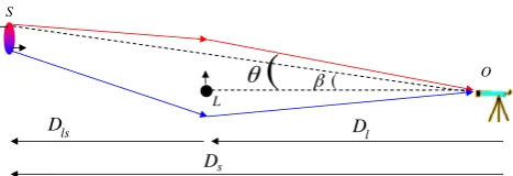
Table 1. Input parameters used for Fig.4. The source galaxy is assumed positioned so as to maximize the MCE (i.e. it is separated from the lens on the sky along the direction of motion of the lens, which is clear from images). The lens mass should roughly correspond to the subcluster in the Bullet. A flatCDM cosmology is adopted (Planck Collaboration XVI2014).
Parameter Meaning Value
H0 Present Hubble constant 67.3 km s−1Mpc−1
m Present matter density 0.315
Dl (Angular diameter) 0.945 Gpc
Distance to lens atzl=0.296
Ds Distance to source atzs=1.7 1.795 Gpc
Dls Distance to source from lens 1.341 Gpc
position in space–time
M Mass of lens 1.2×10¹⁴M
rd Scale length of source galaxy 3.068 kpc
vt Tangential velocity of lens 3000 km s−1
vf Flat line level of source galaxy 100 km s−1
rotation curve
sinicosγ See Fig.2and equation (21) 1 2
Using parameters appropriate to the Bullet Cluster (Table1), the effect is around 1 km s−1.
3.2 Source and observer motion
The peculiar velocity (with respect to the CMB) of the Sun is well known (369 km s−1; Planck Collaboration XXVII2014) and could be included in a more careful analysis. We do not include it as we only seek a rough idea of the magnitude of the MCE. This will not be substantially affected by observer motion as this is much slower than that of the lens (∼3000 km s−1).
More problematic may be the unknown peculiar velocity of the source. Treating the Local Group peculiar velocity (∼630 km s−1) as typical for galaxies, the Bullet Cluster transverse motion likely greatly exceeds the source’s peculiar velocity. In this case, only the component of this velocity parallel to the lens transverse motion has much effect on image redshifts, leading to a factor of1
2on average. 2
Another factor of 1+zl
1+zs
Dl
Ds ≈
1
4arises due to the geometry of the situation and cosmic expansion. Moreover, typical peculiar veloci-ties were smaller long ago. Supposing they were12as much as today atzs=1.5, we see that source motion cannot affect the inferred lens velocity much more than∼50 km s−1. This effect can be reduced by observing more than one double image pair. However, we consider the accuracy with even just one well-observed pair sufficient.
Thus, we ignore any motion other than that of the lens. We note that it might be good to avoid source galaxies which are interacting, as their peculiar velocities might be higher.
3.3 Cosmological expansion
A redshift difference between the images can also arise because the time of flight of photons emitted by the source is different depending on which path they took to get to the Earth. As the photons for both images arrive simultaneously, the photons for one image must have been emitted earlier than for the other. Thus, in an expanding Universe, one of the images will have a higher redshift. Because of both a longer path length and a stronger gravitational
2For an angle between a fixed vector and another statistically isotropic one, |cosθ| = 1
2.
at University of St Andrews on March 31, 2016
http://mnras.oxfordjournals.org/
field along the path, this image is the secondary (on the opposite side of the lens as the unlensed source would appear – see Fig.1). We term this the differential expansion effect (DEE).
A quick way to estimate the DEE is to assume that cosmological distances likeDLare usually∼Hc. The extra path length∼DLθ2. The effect of the difference in gravitational time delays can crudely be approximated as equal to that due to different geometric path lengths.
The DEE expressed as a redshift=H t≈θ2. Meanwhile, the MCE∼vcθ. Assuming a velocity of 3000 km s−1 and an image separation of 20 arcsec, we see that the MCE is∼50 times larger than the DEE. Thus, we calculate the DEE more precisely.
We first consider just the difference in time of flight (‘delay’) due to different strengths of gravity along the two possible photon paths (Shapiro1964). The relative Shapiro delay between the images is
tl= 4GM
c3 ln b
2 b1
,Ds, Dlsb1,2. (14)
The impact parameters of the rays areb1, 2. This result is valid ifb
is much larger than the Schwarzschild radius of the lens, so the rays are only weakly deflected. The ray with smallerbis delayed more as it goes deeper into the lens’ gravitational potential well. It also has a longer geometric path length (it forms the secondary image in Fig.1).
Note this is the time delay at the lens. In reality, both photons must reach the Earth now, so the time of emission at the source must have been different. This requires an extra factor of the relative rates of a clock at the lens and at the source, 1+zl
1+zs.
We then combined this Shapiro delay with the geometric path difference between the trajectories. Thus, the difference in time of emission required for photons traversing the two trajectories to reach the Earth simultaneously is
ts
= 1+zl 1+zs
2GM c3
u u2+4+2 ln
u2+u√u2+4+2 2
.
(15)
We used equation (10) to relate the source positionuto the positions of its images. A correction for cosmological time dilation was also applied.
The change in redshift is given by the fractional difference in the scale factor of the Universe at the time of emission of the photons:
z=H(zs) ts. (16)
Using realistic parameters (Table1andu≈1), the DEE∼1 m s−1. In Section 3.1, we showed that the MCE is∼1000 times larger, allowing us to neglect the DEE.
Even with more accurate instruments, a very large number of double image pairs would need to be observed before the random noise from source peculiar motions was reduced below such a small level. Thus, the DEE will not be important in the foreseeable future. An exception might possibly arise if the source galaxy peculiar motion could be estimated based on properties of galaxies near it.
4 D E R I VAT I O N O F T H E D I F F E R E N T I A L M AG N I F I C AT I O N E F F E C T F O R U N R E S O LV E D I M AG E S
[image:5.595.310.549.57.150.2]The effects mentioned in Section 3 cause the frequencies of identical photons emitted in different directions to end up different when
Figure 2. The observing geometry is shown here. The source galaxy has centre O and normal to its planeO N. Earth is towardsO E, so the galaxy’s inclination to the sky plane isi.O QandO Pare in the galaxy’s plane and orthogonal to each other, withO Qas closely aligned withO Eas possible. Thus,O PandO Eare orthogonal.∇Ais directed within the source plane, so must also be orthogonal toO E.∇Ais at an angleγtoO P. The source is parametrized using cylindrical polar coordinates (r,φ), with centreOand initial direction (φ=0) alongO Q.
measured at the Earth. The DME does not do this. It is merely an observational artefact due to inability to simultaneously resolve the images and take highly accurate spectra of them. This causes parts of the source with different redshifts to get blended together in the spectra. The precise way in which this blending occurs is different between the images.
We assume the spectra are integrated over the entirety of each image. The source is modelled as a typical spiral galaxy with ex-ponential surface density profile and a realistic rotation curve. The lens is treated as a point mass. The parameters considered (Table1) are designed with the Bullet Cluster (Tucker et al.1995) in mind.
The basic idea is that spatially unresolved spectra can determine the intensity-weighted mean redshift of each image. This may be affected by rotation of the source galaxy. The effect is not reliant on an expanding Universe, so it will be simplest to think of the Universe as static for the remainder of this section.
The mean redshift velocity of each image is given by
vr≡
ImageAvrdS
ImageAdS
. (17)
The integrals are over area elements of the sourceS. This is treated as a disc with surface density
=0e− r
rd. (18)
The magnification Avaries little over the source galaxy. This is because rd
Ds θE(see Table1). Thus, a linear approximation toA
is sufficient:
A≈A0+
∂A
∂udu (A0≡Aat centre of source). (19) In our model,Avaries linearly with position in the source plane, but only in the direction directly away from the (projection of the) lens. In the orthogonal direction,Ais independent of position at first order (becauseuis, andAdepends only onu).
The geometry of the source is shown in Fig.2. The radial velocity of any part of it is
vr=vc(r) sinφ sini. (20)
Only the component of∇AalongO P is important. To see why, suppose that ∇A was entirely along O Q. Reflecting the galaxy about the lineOPwithout altering∇Ashould reverse the DME as this is equivalent to reversing∇A. However, the radial velocity of every part of the galaxy remains unaltered after the reflection (asφ →π−φ). Thus, the DME must also remain unaltered.
at University of St Andrews on March 31, 2016
http://mnras.oxfordjournals.org/
[image:5.595.53.286.419.470.2]Noting that the component of∇AalongO Nis irrelevant for the DME, we see that only the component alongO Pmight be relevant. This component causes the approaching and receding halves of the galaxy to be magnified differently. It will be responsible for the DME. Thus, we assume the lens is located somewhere along the lineO P, making∇Aentirely along this direction. The result is then multiplied by cosγ.
The magnitude of the DME is therefore∝cosγsini. Assuming isotropy, all values ofγare equally likely. But values oficlose to
π
2 are more likely because there are more ways for two vectors to be orthogonal than to be aligned. This means the ratio between the average magnitude of the DME and the maximum it could be is given by the mean of|cosγsini|, withγunweighted but a further siniweighting overi.3Thus,
|sinicosγ| = π
2
0 cosγdγ π
2
0 dγ π
0 sin 2idi π
0 sinidi
= 1
2. (21)
The angular separation between the lens and the unlensed source is given by
u=u0+ r.O P
DsθE
(u0≡uat centre of source). (22)
The component of r (measured from the galaxy’s centre) along O Pisrsinφ. We have not kept careful track of signs because, for any conceivable orientation, the source galaxy could be rotating in the opposite sense, thereby reversing the DME. We explain which image has a lower redshift due to the DME later.
The difference inubetween the centre of the source galaxy and any other point in it is given by
du= r sinφ DsθE
. (23)
A0represents a constant magnification across the source. This does not contribute to the numerator in equation (17) because the radial velocityvr∝sinφ, whileis independent ofφdue to axisymmetry. Thus, integrating overφgives 0.4The DME arises when including the first-order correction toA.
The denominator in equation (17) is a normalization for each image (its total intensity).5 Because the magnification is nearly constant across the source galaxy, we can approximate thatA = A0. The first-order correction toAwould have a sinφdependence, which is irrelevant when integrated over allφ. This further justifies our approximation. Therefore, the denominator in equation (17) becomes
Image
AdS=0πrd2
u2+2 u√u2+4±1
. (24)
To understand the sign of the DME, first note that regions closer to the lens are magnified more. In our approximation, the numerator in equation (17) is determined by ∂∂Au, which is the same for both
3Edge-on galaxies are less likely to be detected due to dust obscuration.
This makes low values ofi– and thus a smaller DME – more likely, for a randomly selected multiple image.
4This is expected, as the DME does not arise if the image is uniformly
magnified.
5What we perceive as the total intensity givenD
s andzs, but without
correcting for magnification by the lens.
images (equation 12). Therefore, the image with the lower magnifi-cation (the secondary image) has a larger|vr|. Thus, if it was known which side of the rotating source was the approaching side, one could determine which image should have a higher mean redshift due solely to the DME.
Including the second-order dependence of A on sky position slightly alters the calculations done so far. Because a second-order term does not affect the approaching and receding halves of the source galaxy differently, the numerator in equation (17) is unal-tered. But the denominator is affected, because the total intensity of each image may be altered by a second-order term. This means that our derivation of the DME has a fractional error which is second order in rd
DsθE. We consider this acceptable and proceed to develop
a model for the redshift structure of the source. This requires a rotation curve.
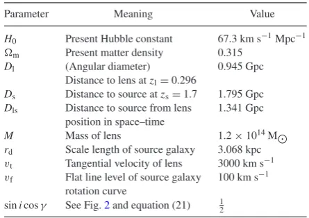
4.1 Model rotation curves
It will likely be difficult to directly observe the source galaxy rota-tion curvevc(r) as it is very far away. It is also difficult to precisely determine its surface density and thus predict the form ofvc(r). Fortunately, we are considering a disc-integrated spectrum and so the exact shape ofvc(r) will turn out not to be very important once the maximum levelvmaxis fixed.
To get a rough idea ofvc(r), we take advantage of the tight empir-ical relation between the forces in rotating disc galaxies as required to sustain their rotation curves and those predicted by Newtonian gravity based on the visible (baryonic) mass (Famaey & McGaugh 2012, and references therein). This empirical formalism goes by the name of modified Newtonian dynamics (MOND; Milgrom1983). Regardless of whether it is correct at a fundamental level, it does seem to provide a good empirical way of predicting rotation curves. Here, this is important because measuring the actual rotation curve of the source galaxy would be very challenging.
The particular empirical relation we adopt follows the work of Famaey & Binney (2005):6
|g|
|g| +a0
g=gN, (25)
where g is the true gravitational field strength while gN is the prediction of Newtonian gravity based on the visible mass.a0is an acceleration scale (≈1.2×10⁻¹⁰m s−2) below which either gravity becomes non-Newtonian or DM must be considered in addition to the baryons. Thus, the magnitude of the gravitational field is given by
g= gN 2 +
gN 2
2
+gNa0. (26)
It is not worthwhile to accurately determinegNfor any particular mass distribution because the actual mass distribution in the source is uncertain. Thus, we approximatedgNusing an analytic method. We assumed that, to determinegNat a particular in-plane location, only material at smaller radii need be considered (we verified that the force from material at larger radii was very small). The Newtonian force at a distancerfrom the centre of a narrow ring of mass dM
and radiusxis
gN≈ GdM
r2 +
3GdM x2
4r4 (x < r,interior ring). (27)
6This is the so-called ‘simpleμ-function’ in MOND.
at University of St Andrews on March 31, 2016
http://mnras.oxfordjournals.org/
This is correct at second order in xr. The total force at any point within the disc was found by decomposing the galaxy into a large number of rings with dM=2πxdx (x). We then summed only the forces resulting from interior rings. Therefore,
gN= r
0 G
dM r2 +
3GdM x2 4r4
(28)
=2πG0f(r), where (29)
r≡ r rd
and (30)
f(r)= 1− 13
4 e−r
r2 −
7 e−r 4r +
91−e−r−re−r
2r4 . (31)
When obtaining the true value ofgfromgN, the ratiogN
a0is important.
Therefore, we introduce a new variable, the dimensionless density
k,
k≡ G0 a0
. (32)
Typical values forkare order 1. Using the empirical equation (26) to getgfromgN:
g a0
=πkf(r)+πkf(r)+12−1. (33)
To get the rotation curve, we equategwith the centripetal acceler-ation. Thus,
v2 c r rd
= g
a0
a0, (34)
vf =
4
√
2πk√rda0. (35)
The rotation curve flat lines at the levelvf= 4 √
GMa0, where the total disc massM=2π0rd2. The shape of the rotation curve is given by
vc(r)≡ vc(r) vf
=
πkrf(r)+rπkf(r)+12−1
4
√
2πk . (36)
We show two such rotation curves in Fig.3. Here, we also show howKaffects the ratio betweenvmaxandvf.
4.2 The final result
Combining our results, we get that
|vr| =
vfrdsinicosγ DsθE
× ∞
0 2π
0
∝
e−r vc(r)r2
−∂A ∂u
4 u2(u2+4)32
sin2φdφdr
π
u2+2 u√u2+4±1
∝A
. (37)
The magnificationAchanges by order 1 over an angular distance ofθE, while the angular radius of the source galaxy ∼rd
Ds. Thus,
[image:7.595.312.542.60.377.2]the DME as a fraction of the typical radial velocity of the source
Figure 3. Top: rotation curves resulting from equations (31) and (36), used in this work.vc(r) flat lines atvf. The surface density=0e−
r rd. The parameterkcontrols the shape of the rotation curve (k≡ 0G
a0 ). Bottom: the
ratio of maximum to flat line rotation speed as a function of central surface density.
is∼ rd
DsθE. The galaxy’s typical radial velocity is vfsini. Another
factor of cos (γ) is needed to account for the lensing geometry. As can be seen from equation (37), this provides a rough guide to the DME (asu∼1 for a realistic target).
An important quantity for the DME is the difference in 1 A∂∂Au between the images:
1 A
∂A
∂u
= ∂∂Au
1 A
= √ 4
u2+4. (38)
In equation (37), the integration overφyieldsπ. The integral over
ris not analytic. Thus, we define
I≡ ∞
0
e−rvc(r)r2dr. (39)
Substituting forθEusing equation (8), we get that
vr|DME=
vfrd sinicosγ I c √
Dl √
u2+4√GMD lsDs
. (40)
The integralIdepends somewhat on the central surface density in the sense that, for the samevf, the DME is greater at higherk. However, themaximumrotation speed is very well correlated with the DME. In fact, the ratiovI
max =1.89±0.02 fork=0.1→5. As
maximum rotation speeds are generally easier to determine than the flat line level, this makes correcting for the DME easier.
If the surface density declines sufficiently slowly withr, then the integralImight diverge. This is due to limited validity of a linear
at University of St Andrews on March 31, 2016
http://mnras.oxfordjournals.org/
approximation toA– a more careful treatment would be required. This might apply to rotating elliptical galaxies withρ∝r−4. But even if∝r−3, the divergence ofIis fairly slow. Thus, although the integral would need a cut-off radius, its precise value would not affect the result much.
A linear approximation toAmust break down ifuchanges by order 1. Thus, a logical cut-off might be the Einstein radius (at the source plane) or the distance between the source and the projected lens.
If a fibre-fed spectrograph was used or the field of view was otherwise restricted, then this may impose an obvious cut-off. For an inclined disc galaxy, a circular aperture would cover a non-circular region in the disc plane. One might need to take this into account.
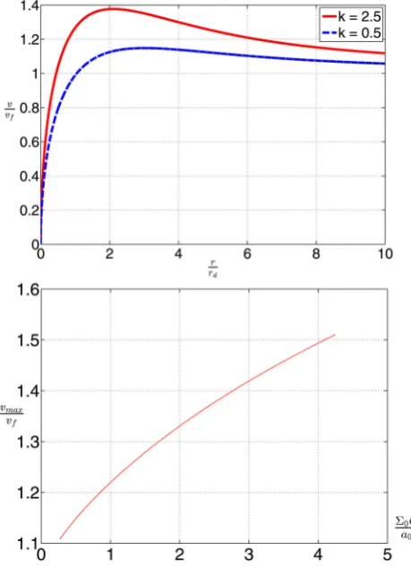
We now decide on realistic parameters to gain a feel for the scale of the DME and MCE. Ideally, one would like to measure the motion of both components of the Bullet Cluster. However, we choose a mass corresponding roughly with the subcluster in the Bullet (Mastropietro & Burkert2008). This is because the centre of mass likely has little peculiar velocity as there is little structure on such large scales. Thus, the lower mass component probably moves faster (with respect to the Hubble flow).
The MCE∝v√M(equation 13). Assuming also thatv∝ 1 M for the components of the Bullet Cluster and that the value ofuwould be broadly similar whichever component is targeted, the MCE overall ∝ √1
M. This makes it larger around the subcluster. Furthermore, using its motion to extrapolate the total collision velocity is much more reliable than using the motion of the main cluster, because the subcluster contributes most of the relative velocity.
A typical source galaxy orientation is chosen using equation (21). Although we usedvf=100 km s−1, it is around double this for our own Galaxy (e.g. McMillan2011).
Using the parameter values in Table1, we obtained the results shown in Fig.4. The DME and MCE are comparable in magnitude. Observing a similar source multiply imaged by the higher mass component instead does not reduce the relative importance of the DME. This is because the DME ∝ √1
[image:8.595.45.281.498.664.2]M (equation 40), just like the MCE. In fact, this scaling highlights an additional problem: substructure in the lens (e.g. individual galaxies) with much less
Figure 4. The difference in redshift between double images of a typical background galaxy as a function of its position, due to the effects described in the text (equations 13 and 40). Parameter values used are listed in Table1. The shape of the rotation curve (k) has a modest impact on the DME once its flat line levelvfis fixed. If insteadvmaxis held fixed, then the impact of
kon the DME is very small.
mass than the entire cluster can enhance the DME. For example, an elliptical galaxy in the lens plane withM=1013M
would cause a DME∼3 times larger than the smooth cluster potential.
This problem could be mitigated to some extent by not select-ing images which show indications of beselect-ing lensed by small-scale structure (e.g. avoiding images appearing near a galaxy in the lens plane). We have implicitly assumed that such a selection has been done, such that a point mass model for the lens is appropriate. Even in this case, it might well be necessary to correct for the DME. This correction would be less relevant if targets could be selected for which the effect is small. We now consider how these things might be achieved.
5 C O R R E C T I N G F O R T H E E F F E C T
For spatially unresolved spectra, it is possible to calculate the DME by determining the parameters in equation (40). If radial velocities accurate to a few km s−1are obtained for a galaxy, then determining vmaxsinito∼10 km s−1should be feasible using widths of spectral lines (see later).
rdmight be obtained from an image of the target, once distortion and magnification by the lens were corrected for. If the image were taken at more than one wavelength, it would suggest a value fork
(which we do not need very accurately) as the colour can be used to estimate the baryonicM/L.
There is no need to determine the inclination as we are only interested in redshift gradients across the source. However, the ori-entation of the major axis of the image is important in determining the axis of rotation and thus the angleγ in Fig.2.
To know the sense of rotation (i.e. which side of the source galaxy is the approaching side), we would need spectra of different parts of the source galaxy. Naturally, a disc-integrated spectrum would be insufficient for this purpose. However, one could make do with poorer spectral resolution.
The secondary image is inverted relative to the primary, providing an important consistency check if both images were used for such a determination. We strongly recommend doing this, because an error would lead to a 200 per cent error in the calculation of the DME. The chance of this is minimized with two determinations of the sense of rotation.
Finally, we also need∇A, which must come from a lensing re-construction.
5.1 Additional information from detailed spectral line profiles
It is often possible to extract more information from a spectral line than just the location of its centroid. The width of the line profile can be used to estimate e.g.vmaxsini.
The MCE simply shifts the entire spectrum. The DME leads to a ‘tilt’ being introduced because one side of the galaxy is magnified more than the other. These effects are different. Therefore, detailed line profiles can tell us if the shift in the centroid of spectral lines is due to the MCE or the DME. This would avoid the need to determine parameters like the disc scale length and orientation. A detailed lensing reconstruction to determine∇Awould also be avoided.
We investigate how the DME and MCE affect line profiles of disc galaxies with rotation curves parametrized by equation (36). We assume the galaxy is viewed edge-on, so the radial velocity of any part of it is
vr(r, φ)=vc(r) sin(φ). (41)
at University of St Andrews on March 31, 2016
http://mnras.oxfordjournals.org/
Figure 5. Radial velocity map of a disc galaxy viewed by an observer within its plane at largex, for the casek=2.5. Radial velocities are antisymmetric about thex-axis. The radial coordinate is rescaled so all parts of the figure would be equally bright. The units are such thatrd=1 andvf=1. Note the
large region withvrclose to the maximum value. The result fork=0.5 is
very similar, althoughvmaxis much closer tovf.
The resulting radial velocity map is shown in Fig.5. Only half of the galaxy is shown becausevris antisymmetric about the viewing direction (thex-axis). vr is symmetric about the y-axis, because sinφ=sin (π−φ).
To determine the profile of a narrow spectral line, we divide the galaxy up into a large number of elements. We use cylindrical polars sovrbecomes separable. Thus, the rotation speed only needs to be calculated once at eachr(for allφ). The radial velocity at the centre of each element is used to classify it among 200 bins in radial velocity.
Assuming constant mass-to-light ratio (M/L) for the baryons, the total intensity of the element multiplied by the magnificationA
is then assigned to the corresponding radial velocity bin. Because radial velocities and wavelengths are directly related, in this way one obtains a synthetic line profile.
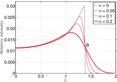
Spectral lines have an intrinsic width and can be further broad-ened by random motions within the galaxy. To account for these effects and also for instrumental errors, we convolved our synthetic line profiles with Gaussians of various widthsσ. The results are shown in Fig.6. The sharp peaks atvr≈ ±vmaxsinigive rise to the name of a double-horned profile.
These horns are caused by the rotation curve having a peak, leading to a small range invrcorresponding to a large range inr. The greatest attained values of|vr|also correspond to large ranges inφ, because sinφis nearly independent ofφwhenφ≈ ±π2.
Thus, a small range invrcorresponds to a large region in the galaxy. Moreover, the peak rotation speed occurs at a radius close to that which maximizes the light emitted per unit radius (r=rd). Fig.5shows the ‘bull’s eye’ corresponding to the fairly large region with near-maximal|vr|. This is responsible for the very pronounced horns in the line profile. They are somewhat less pronounced at highσ.
[image:9.595.59.277.58.192.2]Although one might expect a feature corresponding to vf (at least at lowσ), this is absent. A quick look at Fig.5shows why vc(r)≈vfonly for sufficiently larger. There is very little light from such regions, so a disc-integrated spectrum is hardly sensitive to them. In fact, due to the steep decline in surface brightness withr, most of the spectral intensity atvr=vfactually comes from the rising part of the rotation curve (whenvcsinφ= vf) rather than from the flat part. Thus, in the line profile, there is nothing special aboutvf. This is not true forvmax.
Figure 6. The synthetic line profile of an intrinsically narrow line in an unlensed galaxy withk=2.5, viewed edge-on. The profile is symmetric aboutvr=0. Velocities are scaled to the flat line levelvf. The sharp drop in
the line profile (blue) would probably get blurred (e.g. by random motions), so we convolved the profile with Gaussians of widthsσ. The results are shown as red lines with thicknesses∝σ. Notice how all four profiles pass close to the point markedB. The result fork=0.5 is similar, if the profiles are scaled to have the samevmaxrather thanvf.
Determiningvmaxsinifrom a line profile is non-trivial as the horns move to lower|vr|asσ increases. Instead of using the horn positions, one could use the values ofvrwhere the intensity is a certain fraction of the intensity at the line centre (vr=0). If this fraction is chosen carefully, then one could simply scale the resulting vrby a constant factor and accurately recovervmaxsiniover a wide range inσandk. To see why, note that spectra with differentσall pass close to the point markedBin Fig.6.
Ultimately, it might be better to compare the observed line profile with a suite of synthetic profiles built for a range of k, σ and vmaxsini. The initial guess forσ might come from considering the shape of the tail. Ifvmaxsiniis accurately recovered, then the DME hardly depends onk.7
The horns are cause by a relatively small part of the galaxy but they greatly affect the mean radial velocity of its image. Thus, if the galaxy was not axisymmetric and e.g. had a dusty spiral arm obscuring light from this region, then the redshift measurement of each image may be biased. Partly for this reason, it may be a good idea to consider the rest of the line profile and not just the mean redshift (which is basically the same as considering just the horns).
We now consider how the DME and MCE affect the line profile. The mean redshift velocity of the line is raised by 1 per cent ofvmax (1.08 per cent ofvffork=0.5 and 1.26 per cent fork=2.5). We consider separately the cases where either the DME or the MCE is wholly responsible for this shift in line centroid. We also construct control line profiles like those in Fig. 6. These are obtained by setting
A=1∀r,φ. (42)
7Line profiles can also be used to findv
fsiniwithout detailed rotation
curves. In this case, the value ofkis important as a ‘correction’ must be applied to get fromvmaxtovf(e.g. bottom panel in Fig.3).kdoes not
affect the line profile much and so it would need to come from an image and photometry.
at University of St Andrews on March 31, 2016
http://mnras.oxfordjournals.org/
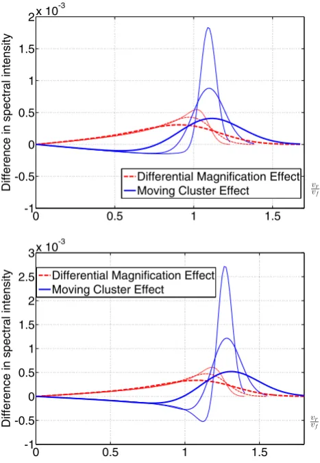
Figure 7. The residuals in the spectral profile due to the DME (equation 43) and the MCE (horizontal shift of profile) are shown here. These were ob-tained by subtracting a control line profile (equation 42). The patterns are antisymmetric aboutvr=0. Results are for an edge-on galaxy withk=
0.5 (top) andk=2.5 (bottom). Both effects change the mean redshift by 1 per cent of the maximum rotation speed, representing 1.08 per cent ofvf
fork=0.5 and 1.26 per cent fork=2.5. The spectra were convolved with Gaussians of widths 0.05, 0.1 and 0.2vf(higherσindicated by thicker line).
The MCE cannot change the amplitudes of the horns. The DME makes one more pronounced and the other less.
In Fig.7, we show the pattern of residuals (relative to the control) created by each effect. The total line intensity is kept the same for the comparison.
To obtain the corresponding observations, one would need to ac-count for the images having different overall magnifications. Thus, the spectra would have to be rescaled. We assume this can be done perfectly (i.e. the photometry is very accurate).
The MCE corresponds to a horizontal shift in the spectrum rel-ative to the control. This means the amplitudes of the horns are unaffected.The pattern of residuals corresponds to the gradient in the spectrum. Thus, the residuals are largest near the positions of the horns, but small precisely at them. The residuals are of oppo-site signs on either side of each horn because the gradient in the spectrum changes sign there.
For the DME, we set
A=1+nrsinφ. (43)
Note that no assumptions are made about any of the factors con-trolling the amplitude of the DME, beyond it being a small effect relative tovmaxsini(i.e.n 1) and that we need not consider the
second-order dependence ofAon position in the source plane. The purpose here is to illustrate how the DME affects the line profile, not how much (this is controlled byn). If the DME∼0.01vfsini, then the residuals would be∼1 per cent of the line profile.
The image overall is not magnified for any (small)n. We adjust
n until the line centroid shifts by the correct amount, to allow comparison with the MCE.
The DME causes one side of the galaxy to be magnified more than the other. Thus, the residuals due to it are of the same sign for each half of the galaxy (e.g. forvr>0). There is no change in sign at the horns.
These correspond to material displaced from the centre of the galaxy along the directionO Pin Fig.2. As argued previously, we only need to consider the component of∇Aalong this direction. Thus, the effects of differential magnification are substantial for the material corresponding to the horns (in so far as the DME affects the image at all). This is in contrast to the MCE, which hardly affects the line profile at these positions (because the gradient of the line profile there is 0).
For somevr, the MCE leads to very large residuals if vσ
fsini is low (Fig.7). Thus, observing faster rotating galaxies might make it easier to distinguish between the DME and the MCE (as vσ
fsini
would likely be smaller). However, the DME would be larger and so it would have to be accounted for more accurately.
Detailed profiles of individual spectral lines may therefore help in determining the balance between the MCE and the DME in accounting for redshift differences between multiple images. In reality, a large number of spectral lines would probably need to be stacked. Even then, it seems likely that, in so far as redshift differences between the images are discernible, the cause of such differences can also be determined.
5.2 The second-order effect
For simplicity, we continue assuming the source is located along O P. Thus, regions with high|vr|are magnified more and regions with lower|vr|are magnified less than the centre of the source due to the second-order dependence ofAon position. To investigate what this means for spectral line profiles, we setAto depend quadrati-cally on position along the directionO P. This introduces a sin2φ dependence:
A= 1+nr2sin2φ
1+3n . (44)
A quadratic dependence along the orthogonal direction would give a cos2φdependence. Because cos2φ=1−sin2φ, a second derivative ofAin either direction would affect the line profile in the same way (i.e. the residuals would have the same pattern, up to sign); once any overall magnification was corrected for.
When comparing the spectra, observers would first scale them to have equal intensities. Thus, we must avoid changing the total intensity. This leads to the factor of 1+3nin the denominator of equation (44).
The results are shown in Fig.8. The effect is symmetric invr, so both horns are equally affected. These end up more pronounced in the secondary image than in the primary (in this example).
In reality, both the first- and second-order DME would be present for any given pair of images of the same object. Thus, the residuals would have both an antisymmetric and a symmetric part. However, the latter would likely be very small for cluster mass lenses (except for caustic images).
at University of St Andrews on March 31, 2016
http://mnras.oxfordjournals.org/
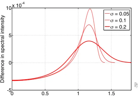
Figure 8. The pattern of residuals for the second-order DME (equation 44) andk=1. A control profile obtained using equation (42) was subtracted and the result convolved with a Gaussian. The residuals are symmetric about vr=0, so both horns become more pronounced in this example.
5.2.1 Non-rotating sources
We briefly consider how the DME might affect a non-rotating pressure-supported galaxy, such as an elliptical. If a galaxy is sym-metric such thatρ(r)=ρ(−r) andσ(r)=σ(−r), then at first order the DME does not affect an unresolved image at all. To see this, con-sider an inversion mappingr→ −rwhile leaving∇Aunchanged. The situation is identical to reversing the direction of∇Ainstead, so one expects the DME to act in exactly the opposite way on the spectrum. But the situation has not physically changed, so the DME must also remain unchanged.
This conclusion breaks down at second order. Suppose parts of the galaxy further from its centre are magnified more. Then, as the velocity dispersion generally decreases outwards, the derived velocity dispersion of the image will be reduced by the DME. The effect is larger for the fainter (secondary) image, which will thus appear to have a smaller velocity dispersion than the primary in this example.
This is likely to be more important for galaxy–galaxy lensing as θEis smaller, making duover the source larger. In this case, the DME might be useful to constrain the form ofσ(r) using a double image of a distant elliptical galaxy.
Alternatively, if the source galaxy was well understood, one might be able to constrain∇Aand thus have a better understanding of the lens. Doing both simultaneously would likely be very challenging and model dependent.
6 TA R G E T S W I T H A S M A L L E R E F F E C T
Fig.4shows that the DME may well need to be accounted for when using the redshifts of double images to determine the motion of the lens. However, doing this accurately may be difficult because of the cosmological distance to the source galaxy. Therefore, we suggest sources for which the DME should be smaller, allowing us to correct for it less accurately.
Some strategies outlined here involve selecting targets which are harder to observe, thereby making their spectra less accurate. It is up to observers to decide which targets best minimize the uncer-tainty introduced by the DME while still being feasible to obtain accurate spectra for. We also note that minimizing the uncertainty introduced by correcting for the DME is not necessarily equivalent
to minimizing the magnitude of the DME, because there may be sources for which the DME can be estimated more reliably.
6.1 QSOs
The DME ∝rv, where the source has typical size r and radial velocity spread v. For a given massM, the Virial theorem gives v∝ √1
r. Thus, the DME∝ √r
. For sources with a particularM, the DME would be reduced if the source were smaller, even though it would spin faster.
One obvious type of very small target visible over cosmological distances is a quasi-stellar object (QSO). If a doubly imaged QSO could be found lensed by the Bullet Cluster, it might make an excellent target.
QSO spectra can sometimes lack distinctive features which are required for precise redshift measurements. The Lyαforest might provide a solution, but only if the same feature appeared in both im-ages. Because the rays of light corresponding to the images diverge from the source,8this is only feasible if the gas cloud causing the absorption feature was located fairly close to the QSO.
Another problem might be that the small size of QSOs makes their radiation time variable. Thus, the time delay between the im-ages could make it difficult to compare their spectra. This might require observers to wait out the time delay, which would first have to be determined (though it could be estimated, perhaps using equa-tion 15).
6.2 Smaller and fainter galaxies
The DME is proportional to both the rotation velocity and the size of the source galaxy. Brighter galaxies generally rotate faster (Tully & Fisher1977), so targeting fainter galaxies might help. One advan-tage of this approach is that the number density of fainter galaxies is greater than for brighter ones (Schechter1976). This makes it more likely that suitably oriented multiple images can be found.
However, it would be harder to obtain accurate spectra – and thus redshifts – for fainter targets. Given the high accuracy required in the redshift measurements and the cosmological distance to the source, this is perhaps not the best option at present.
6.3 Elliptical galaxies
Elliptical galaxies might make good targets as they usually rotate slower than spirals, if at all. They might be distinguished using colour or image shape (though one might need to correct for distor-tion by the lens). The surface brightness declines outwards much more gradually for ellipticals than for spirals, potentially providing another way of finding them.
Before conducting detailed observations, targets selected like this might be followed up to check if the spectral line profiles were double horned (characteristic of rotation along the line of sight). A good target should have a Gaussian-looking line profile, characteristic of a pressure-supported object.
However, even ellipticals can rotate, so the DME might not be eliminated by observing one. Also, most galaxies are not elliptical, so finding a bright doubly imaged one is somewhat dependent on luck. Nonetheless, we consider this the best option. This is partly because the work of Gonzalez et al. (2009) identified a multiply imaged galaxy which may be a good target for determining the MCE.
8By an angle 1+zl 1+zs
Dl
Dls(θ1−θ2).
at University of St Andrews on March 31, 2016
http://mnras.oxfordjournals.org/