Preprint typeset in JHEP style - HYPER VERSION
Constraining Disformally Coupled Scalar Fields
Philippe Brax
Institut de Physique Th´eorique, CEA, IPhT, CNRS, URA 2306, F-91191 Gif/Yvette Cedex, France
E-mail: [email protected] Clare Burrage
School of Physics and Astronomy, University of Nottingham, Nottingham, NG7 2RD, United Kingdom
E-mail: [email protected]
Abstract: Light scalar fields can naturally couple disformally to matter fields. Static,
non-relativistic sources do not generate a classical field profile for a disformally coupled scalar, and so such scalars are free from the constraints on the existence of fifth forces that are so restrictive for conformally coupled scalars. In this work we show that disformally coupled scalars can still be studied and constrained through their microscopic interactions with fermions and photons, both in terrestrial laboratories and from observations of stars. The strongest constraint on the coupling scale comes from mono-photon searches at the LHC and requiresM &102 GeV.
Contents
1. Introduction 2
2. Disformally Coupled Scalar Fields 3
2.1 Effective Action 3
2.2 Absence of Tree Level Interactions with Static Non-Relativistic Sources 4
2.3 Interactions with Fermions 5
3. Collider Constraints 6
3.1 Unitarity 7
3.2 Constraints from Searches for Beyond the Standard Model Physics 7
4. The One-Loop Fifth Force 8
4.1 Constraints from Fifth Force Experiments 11
5. The Scalar Casimir and Casimir-Polder Effects 11
5.1 The Disformal Force in a Plate-Sphere Casimir Experiment 12 5.2 The Disformal Force in a Casimir Polder Experiment 12
6. Constraints from Precision Atomic Measurements 14
7. Neutron Scattering Experiments 15
8. Constraints from Stellar Burning 16
8.1 The Scalar Mean Free Path 17
8.2 Unitarity Constraints 18
8.3 Bremsstrahlung 19
8.4 Compton Scattering 21
8.5 Primakov Process 23
8.6 Pion Exchange 25
9. Summary and Conclusions 27
9.1 Summary of Constraints 27
1. Introduction
Are we allowed to introduce a new light scalar field [1] that couples to matter [2]? For conformally coupled scalar fields, the answer to this question appears to be “yes, but with difficulty”. If a scalar field has a canonical kinetic term, and its potential consists only of a mass term, then experimental searches for fifth forces severely constrain the existence of a minimal coupling to matter [3]. These constraints can be alleviated through screen-ing mechanisms that introduce non-linear, higher order operators (that can be radiatively stable) but the cost is a more baroque scalar sector. Disformal couplings present an inter-esting alternative; such a coupling does not (classically) result in a force between static, non-relativistic objects and therefore is not constrained by the fifth force experiments that are so restrictive for conformal couplings.
Disformal interactions were first discussed by Bekenstein [4], who showed that the most general metric that can be constructed from gµν and a scalar field that respects causality and the weak equivalence principle is;
˜
gµν =A(φ, X)gµν+B(φ, X)∂µφ∂νφ , (1.1)
where the first term gives rise to conformal couplings between the scalar field and matter, and the second term is the disformal coupling. Here X= (1/2)gµν∂µφ∂νφ. The disformal interactions give rise to Lagrangian interaction terms of the form
L ⊃ 1
M4∂µφ∂νφT
µν . (1.2)
where Tµν is the energy momentum tensor of matter fields. As is clear from Equation (1.2) a disformal coupling occurs through a high mass dimension operator, however if the scalar field possesses a shift symmetry then this is the lowest order operator we can write down which respects Lorentz invariance. This direct coupling between derivatives ofφand the energy-momentum of matter is such that the matter density T00 only couples to time derivatives of φ. As a result the scalar field is not sourced by a static pressureless perfect fluid. However, quantum effects are still present and a new force mediated by the scalar field appears at the one loop level [5, 6]; we will examine this force in detail in Section 4. Operators of even higher order than those in Equation (1.2) can be generated by quantum corrections. Those involving additional derivatives of∂µφgive rise to terms in the equation of motion that have more than two derivatives per field and thus are expected to give rise to ghost degrees of freedom. Such terms are suppressed by the cut off of the effective field theory which we expect to lie above the scale M. Other higher order operators contain the same ∂φ∂φT combination, and remain small compared to the term in Equation (1.2) if (∂φ)< M2.
bound on M. Our aim in this work is to determine the best current constraints on the scaleM. A variety of observational probes of disformal couplings have also been previously considered: The disformal interactions of scalars with photons can be probed in laboratory experiments [7]. In models motivated by Galileon theories and massive gravity, constraints have been put on the disformal interactions from studying gravitational lensing and the velocity dispersion of galaxies [8, 9]. A disformally coupled Galileon has been shown to fit current cosmological observations and a non-zero disformal coupling seems to be marginally preferred [10]. Other cosmological implications of disformal scalars have been considered in [11–15]. Disformal interactions have been shown to arise in the four dimensional effective theory resulting from various brane world scenarios [16, 17], in branon models [18, 19] and in theories of massive gravity [20, 21].
In this work we determine the constraints imposed on disformal scalars by consider-ing the microscopic interactions between scalars, fermions and photons. We will find that constraints on the disformal coupling can be imposed by a wide ranging array of labo-ratory experiments and astrophysical observations. In the first section, we introduce the disformal coupling and show the absence of any classical effect in the presence of dense and non-relativistic matter. In Section 3 we consider the constraints imposed on the the-ory by requiring unitary evolution in particle colliders, and then bound the thethe-ory with the null results of mono-lepton searches for new physics at the LHC. Then in Section 4, we investigate the quantum effects and rederive the force between two fermions due to a scalar loop. This force is strongest at short distances therefore in Section 5 we study the macroscopic effects of the disformal interaction and consider the disformal Casimir-Polder interaction between one fermion and a plate, and the disformal Casimir effect. In Section 6 the one loop force is applied to atomic transitions in hydrogen-like atoms where the disformal interaction changes the atomic energy levels. We also calculate the cross section in the scattering between non-relativistic neutrons and rare gases in Section 7. We then check in Section 8 that the disformal interaction does not lead to a fatal increase in the burning rate of stellar structures. We conclude and summarize the constraints in Section 9.
2. Disformally Coupled Scalar Fields
2.1 Effective Action
As discussed in the introduction a disformal coupling between matter and a scalar field,φ, arises because in the Einstein frame matter fields move on geodesics of a metric ˜gµν that depends on the scalar field. We consider a disformal scalar field defined by the following action:
S=
Z
d4x√−g
R
2κ24 −
1 2(∂φ)
2
+Sm(ψi,˜gµν), (2.1)
where the metric is
˜
gµν =gµν+
2
This is not the most general scalar metric as given by Bekenstein in Equation (1.1), however it describes all the leading order effects of disformal couplings, and is much simpler to work with. The coupling scaleM is constant and unknown and should be fixed by observations. The metric ˜gµν is the Jordan frame metric with respect to which matter is conserved
[12] (this follows from diffeomorphism invariance of Sm):
˜
DµT˜µν = 0, (2.3)
where the Jordan frame energy momentum tensor is
˜
Tµν = √2 −g˜
δSm δg˜µν
. (2.4)
The Einstein frame energy-momentum for matter is Tµν = (2/√−g)(δSm/δgµν).
2.2 Absence of Tree Level Interactions with Static Non-Relativistic Sources
The disformal coupling induces interactions between the scalar field and matter at all orders in 1/M4. The first order interaction reads
S(1)= 1
M4
Z
d4x√−g∂µφ∂νφTµν . (2.5)
Higher order terms are simply obtained by iteration
S(n) = 1
M4n Z
d4x√−gCα1β1...αnβn
(n) (∂α1φ∂β1φ). . .(∂αnφ∂βnφ), (2.6)
where we have identified the tensor
Cα1β1...αnβn
(n) = 2n
√ −g
δnSm(ψi,g˜µν) δgα1β1. . . δgαnβn
˜
gµν=gµν
, (2.7)
or equivalently
Cα1β1...αnβn
(n) = 2n−1
√ −g
∂n−1(√−gTα1β1)
∂gα2β2. . . ∂gαnβn
˜
gµν=gµν
. (2.8)
For non-relativistic matter, we have
Tµν=ρuµuν , (2.9)
where ρ is the matter density (which is a delta function for matter particles) and the velocity 4-vector is uµ = dxµ/dτ where the proper time is dτ = (−gµνdxµdxν)1/2. At second order we find that
Cα1β1α2β2 (2) = (g
2.3 Interactions with Fermions
In what follows we will restrict ourselves to the leading order effects of the disformal coupling between the scalar field and matter, and so calculate only to leading order in 1/M4. To this order the action can be expanded as
S =
Z
d4x√−g
R 2κ2
4 −1
2(∂φ)
2+ 1
M4∂µφ∂νφT µν
+Sm(ψi, gµν). (2.11)
whereTµν is now the Einstein frame energy-momentum tensor for matter.
In this paper we will focus in detail on the microscopic interactions between the scalar field and fermions, for which we first need to determine the interaction vertex. A fermion field in the Jordan frame is characterized by the action
SF =−
Z
d4xp−˜g[iψ¯γ˜µD˜µψ+mψψψ¯ ], (2.12)
where the Dirac matrices and the covariant derivatives are those corresponding to ˜gµν. The associated Einstein frame energy momentum tensor is given by
Tψµν=−i 2[ ¯ψγ
(µDν)ψ−D(µψγ¯ ν)ψ], (2.13)
where indices have been symmetrised and we have taken the fermions to be on-shell. There-fore the Einstein frame scalar action contains a disformal interaction with the fermions of the form:
Sφ⊃ −
Z
d4x i
2M4∂µφ∂νφ[ ¯ψγ
(µDν)ψ−D(µψγ¯ ν)ψ]. (2.14)
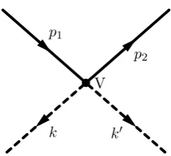
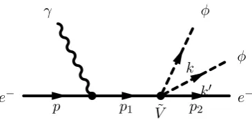
In static situations where the scalar field profile is non-trivial, this implies a modification of the fermion dispersion relation [22] and superluminal effects1. Here we are interested in the quantum properties of this interaction. They can be deduced from the interaction vertex shown in Figure 1:
V =− 1
4M4u¯(p2)[(k.p1)k/ 0
+ (k0.p1)/k+ (k.p2)k/0+ (k0.p2)/k]u(p1), (2.15)
wherep1,2 are the four-momenta of the external fermions.
We now summarize our conventions for the following calculations: We take external Dirac fermions to be normalized such that
X
s
¯
us(p)¯us(p) =−/p+imψ , (2.16)
where the sum is over the spins±1/2. We chose the γ matrices to be in the Dirac repre-sentation corresponding to the mostly plus signature (−+ ++)
γ0 =i
I2 0 0 −I2
!
, γi =i 0 −σ i
σi 0
!
, (2.17)
p1
p2
k k0
[image:7.595.234.357.77.189.2]V
Figure 1: The disformal interaction vertex connecting two fermions (solid lines) and two scalars (dashed lines).
where I2 is the two dimensional identity matrix and the σi’s are the Pauli matrices. This will be convenient when taking the non-relativistic limit of various interactions.
In the non-relativistic limit, we have
us=
p
2mψ ψs
˜ ψs
!
, (2.18)
where ˜ψ = −mψσ.pψ, the 3-momentum of the fermion is pi, and ψs is the non-relativistic wave function of a spin 1/2 fermion. Notice that in this limit we have P
su¯s(p)¯us = mψTr(iI4 +γ0) = 2imψ, where I4 is the 4-dim identity matrix, where the last equality holds for the non-relativistic wave function of the spin 1/2 fermions.
3. Collider Constraints
The interaction vertex shown in Figure1allows a fermion and an anti-fermion to annihilate into two scalars, such interactions typically occur in particle colliders, and the null results of searches for beyond the standard model physics can be used to constrain the disformal interaction. On purely dimensional grounds the cross section for this interaction can be expected to take the form
σ∼α1
E6 M8 +α2
E4m2
M8 +. . . (3.1)
whereEis the center of mass energy,mis the mass of the fermions, andαiare dimensionless coefficients. In [6] it was assumed that the leading term in Equation (3.1) would be the dominant contribution to the cross section, and as a result it was estimated that requiring unitarity for electron-positron collisions at the LEP collider imposes M &200 GeV. Here we show that in fact α1 = 0 and therefore the unitarity constraints on the disformal coupling scale are weaker than previously thought.
The scattering amplitude corresponding to Figure 1is
|M|2 = 1
16M8Tr[X/(−/p1+im)X/(−/p2+im)], (3.2)
where Xµ = (k·p1)kµ0 + (k0 ·p1)kµ+ (k ·p2)k0µ+ (k0 ·p2)kµ. We work in the center of mass frame where the incoming fermions have four-momenta p1 = (E,
√
and p2 = (E,− √
E2−m2~z) and the corresponding scalar momenta are k = (E, ~q) and k0 = (E,−~q), where q~2 = E2 and ~z is a unit vector. We find that the structure of the vector Xµ leads to a cancellation amongst the terms that are independent of the fermion mass and as a result we find
|M|2 = 8m
2E6
M8 . (3.3)
The corresponding cross section is
σ = m
2E4
πM8q1−m2 E2
. (3.4)
At energies higher than the fermion mass the square root can be expanded to put this expression into the form of Equation (3.1), and identifyα1= 0 and α2= 1/4π.
3.1 Unitarity
Clearly the cross section in Equation (3.4) diverges as the energy of the interaction is increased, leading to a violation of unitarity. Particle interactions have been observed to be unitary all the way up to the TeV scale energies probed by the LHC, therefore we require that M . 16π for all observable interactions. With the scattering amplitude of Equation (3.3) we can update the unitarity bounds from LEP; the collider reached energies of 209 GeV when colliding electrons and positrons, for the disformal contribution to these interactions to be unitary we must impose:
M &3 GeV. (3.5)
The LHC now reaches significantly higher energies than were accessible at LEP. Making the conservative assumptions that the most common interactions involve up and down quarks with energies∼2 Tev then we find that unitarity requires
M &30 GeV. (3.6)
Clearly the bounds on M can be increased if heavier particles, or higher energy collisions are considered.
3.2 Constraints from Searches for Beyond the Standard Model Physics
of WIMP dark matter particles in fermion annihilation it is unclear how to translate these bounds into constraints on disformal scalars.
Mono-lepton searches are more easily applied to disformal scalars. The results of searches for new physics in the final states with an electron or a muon was reported by the CMS collaboration in Reference [25] following the strategy of Reference [26]. The cross section for such a process, when the interaction is spin and flavour independent, is constrained to be
σ <0.3 pb, (3.7)
for light scalars. The most common interactions involve up and down quarks, and assuming that the energy carried by these quarks can reach 2 TeV we find that this results in a constraint on the disformal interaction of
M &120 GeV. (3.8)
A stronger constraint has been recently obtained using data from the ATLAS collaboration [27] and by the CMS experiment [28] in the single photon channel with a resulting bound on the disformal coupling 2
M &490 GeV. (3.9)
4. The One-Loop Fifth Force
When a source is static and non-relativistic no field profile is generated classically for a disformal scalar field at any order in 1/M. The absence of a force was also explicitly shown at the level of the classical equations of motion in Reference [7]. In References [5, 6], it was shown that the lowest order one loop diagram would correspond to a force between the fermions of the form
F ∼ m1m2
M8r8 , (4.1)
wherem1 and m2 are the masses of the particles being scattered. Contributions at higher loop order are suppressed when M r > 1. An estimate of the constraints from fifth force experiments in Reference [7] gaveM >MeV. In this section we re-derive these results, and then proceed to constrain the existence of this force with torsion balance measurements. Our derivation of the force will follow the calculation of the Casimir-Polder force presented in the textbook by Itzykson and Zuber [29], and we will quote the main results that are derived there.
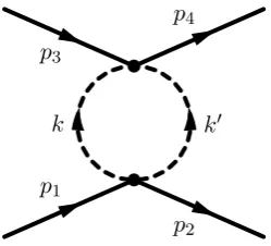
We consider the four fermion interaction mediated by a loop of two scalar fields, as shown in Figure 2. At large distances and in the non-relativistic limit, the Feynman amplitude becomes a function of the momentum transfer
q=p1−p2 , (4.2)
p1 p3
p2
k k0
[image:10.595.234.359.80.193.2]p4
Figure 2: Two fermion scattering mediated by a loop of the disformal scalar field.
where momentum conservation implies that p1+p3 =p2+p4. In this limit we can define the interaction potential between the two fermions as
Vφ(r) =
Z
/
d3qV(q)eiq.r, (4.3)
where we use the standard notation /d3q = (2π)d3q3. This is related to the forward scattering amplitudeF(q2) as
V(q) =i F(q 2)
4m1m2
, (4.4)
where the masses of the two interacting fermions are m1,2.
A convenient way of extracting the small q (and therefore long range) behaviour of V(q) is to notice that, for a fixed Mandelstam variable s=−(p1+p3)2 ≈(m1+m2)2 in the non-relativistic limit, the forward amplitude F is an analytic function of −q2 with a cut along the positive axis3. A dispersion relation then relates FR, the real part ofF, on the positive axis to the forward amplitude
F(q2) = 1 iπ
Z ∞
0
dm2 FR(−m 2)
m2+q2−i , (4.5)
where the Cutkosky rules give
FR(q2) = 1 2
Z /
d3k 2k0 / d3k0 2k00/δ
4
(k+k0−q)d(k, k0)|k2=k02=0. (4.6)
Transforming back to real space we find that the non-relativistic scattering potential is then
V(r) =− 1 16π2m1m2r
Z ∞
0
dm2FR(−m2)e−mr, (4.7)
where the leading order is given by the behaviour ofFR(q2) around the origin and we have q2 = (~q)2.
To perform this calculation for the disformal force it is convenient to define the average
hXi=
R /d3k
2k0 / d3k0 2k00/δ
4
(q−k−k0)X(k, k0)
R /d3k
2k0 / d3k0
2k00/δ 4
(q−k−k0)
, (4.8)
where the denominator is a step function 8π1 θ(−q2). As a result we have that
FR(q2) = 1 16πθ(−q
2)hdi. (4.9)
The scattering amplitude corresponding to Figure 2reads
F(q2) =
Z /
d4k/d4k0 /δ
4
(k+k0−q)
(k2−i)(k02−i)d(k, k
0), (4.10)
where/δ4(k+k0−q) = (2π)4δ(k+k0−q) and dencodes the effects of the two interaction vertices in the Feynman diagram:
d(k, k0) = 1
16M8u¯(p2)[(k.p1)k/
0+ (k0.p
1)k/+ (k.p2)k/0+ (k0.p2)/k]u(p1)
×u¯(p3)[(k.p4)k/0+ (k0.p4)/k+ (k.p3)k/0+ (k0.p3)/k]u(p3), (4.11)
the average of which is
hdi= (q 2)2
30×16×M8[2(p1.p3+p2.p4+p1.p4+p2.p3)¯u(p2)u(p1)¯u(p3)u(p4)
+ ¯u(p2)(p/3+p/4)u(p1)¯u(p3)(p/1+p/2)u(p4)], (4.12)
where we have used the result that, to leading order in q2,
hkµkνk0ρk0σi= (q 2)2
15×16(gµνgρσ+gµρgνσ+gνρgµσ). (4.13)
In the non-relativistic limit
¯
u(p2)u(p1)¯u(p3)u(p4) =−4m1m2 , (4.14)
and
¯
u(p2)(p/3+p/4)u(p1)¯u(p3)(p/1+p/2)u(p4) = 16m21m22. (4.15)
Combining all of the above we find that, in the non-relativistic limit,
FR(q2) = 1 10πθ(−q
2)m21m22(q2)2
16M8 . (4.16)
From which we deduce that the scalar induced interaction between two fermions is
V(r) =− 3
32π3r7
m1m2
M8 . (4.17)
This is an attractive interaction which is proportional to the particle masses.
4.1 Constraints from Fifth Force Experiments
Constraints on deviations from a 1/rNewtonian gravitational potential are most commonly formulated in terms of Yukawa corrections and laboratory experiments aiming to probe such corrections have been performed over a wide range of distance scales from centimeters to tens of nanometers, for a review see [30]. Experiments probing millimeter distance scales give the tightest constraint on the magnitude of the correction to Newtonian gravity, and the constraints weaken dramatically over shorter distance scales.
The best constraints from torsion balance experiments [30] find that the inverse square law holds down to a length scale of 56µm. This requires that the ratio of the disformal potential to the Newtonian potential be less than unity at this distance scale. Such a constraint requires:
0.07 MeV< M . (4.18)
This is a weak bound which will be superseded by other laboratory and astrophysical constraints.
5. The Scalar Casimir and Casimir-Polder Effects
As the disformal one-loop force scales as∼1/M8r8 we still expect the tightest constraints on M to come from experiments performed at the shortest possible distance scales. These short distance experiments are for instance measurements of the Casimir force. The Casimir force is usually discussed as the pressure exerted on the bounding surfaces of a region due to the zero-point fluctuations of quantized fields in the interior. An alternative formulation due to Jaffe [31] describes the Casimir force as the (relativistic, retarded) Van der Waals force exerted between the boundaries of a region. In this formulation, the standard result for the Casimir force is recovered in the α → ∞ limit (a limit that can be shown to be appropriate on the short distance scales used to measure the Casimir effect). The Casimir-Polder effect, closely related to the Casimir force, is the force exerted on a test particle due to a nearby surface. The Casimir force per unit area for two idealized, perfectly conducting plates with vacuum in between then scales inversely with the fourth power of the distance between the platesF ∼1/a4. Therefore experiments searching for the Casimir force focus on probing physics at extremely short distance scales, making them ideal experiments to constrain the existence of a disformal force.
5.1 The Disformal Force in a Plate-Sphere Casimir Experiment
The most sensitive measurement of the Casimir force are those that probe the interactions between a plate and a sphere. To compute the disformal effects in such experiments we have to integrate the interaction over the volume of the sphere and plate. We take the plate to be of density ρ1 and width a with infinite extent in the (x, y) directions. The shortest distance between the plate and the sphere is d and the sphere has density ρ2 and radius R. All experiments are performed with d R. Points on the surface of the plate are described by ~r1 = (r1cosθ1, r1sinθ1,0) and points within the sphere have ~r2 = (r2cosθ2sinφ, r2sinθ2sinφ, d+R −r2cosφ), with 0 ≤ r2 ≤ R. The disformal potential is then found to be
Φ =− 3ρ1ρ2a 32π3M8
Z ∞
0 dr1
Z R
0 dr2
Z 2π
0 dθ1
Z 2π
0 dθ2
Z π
0
dφ r1r 2 2
|~r1−~r2|7/2 , (5.1)
whilst the full integral is difficult to compute it is clear that it is dominated by the con-tribution of the points of closest approach between the sphere and the cylinder. With this assumption, and dR, we can approximate the disformal potential as
Φ =−3ρ1ρ2aR 5
64πM8d7 . (5.2)
The Casimir force between a sphere and a flat surface is
FC = π3R
360d3 , (5.3)
and therefore the ratio of the disformal force,FC =∂Φ/∂d, to Casimir force is
F FC
= 945 8π4
ρ1ρ2aR4
M8d5 . (5.4)
The best constraints on the existence of a disformal force from a Casimir type ex-periment comes from the measurement performed by Lamoreaux [32], where a= 0.5 cm, R = 11.3 cm and ρ1 = ρ2 = 2.6 gcm−3. No deviation from the theoretical prediction of the Casimir force is seen at the 5% level when the plate and sphere are separated by a distances down tod= 0.5 µm. This requires
0.1 GeV< M . (5.5)
5.2 The Disformal Force in a Casimir Polder Experiment
In Section 4 we proved that two point sources are attracted by a disformal potential that scales as the inverse of the seventh power of the distance between the sources. To compute the effect of this disformal interaction in a Casimir-Polder experiment we integrate over a uniform plate. We approximate the experimental environment by assuming that the plate has infinite extent in the (x, y) directions, and that a test particle lies a distancezfrom the surface. We assume that the plate has thickness aand densityρ. The disformal potential experienced by the test particle due to the plate is:
Φ =− 3
32π3 1
M8
Z ρ
whereR2=x2+y2+z2 =r2+z2 and the integral is performed over the plate. Therefore
Φ = − 3 32π3
ρa M8
Z 2π
0
Z ∞
0
r drdθ
(z2+r2)7/2 (5.7)
= − 3ρa
80π2M8z5 . (5.8)
Neutrons in empty space over a thin mirror have quantized energy levels in the ter-restrial gravitational field. The disformal Casimir-Polder interaction between the neutron and the mirror changes the energy levels and the interaction potential
V(z) =m
gz− 3ρa 80π2M8z5
, (5.9)
wheremis the neutron mass. The second term must be a perturbation to the gravitational interaction as the first four energy levels of the unperturbed system have been observed to a precision of 10−14 eV [33]. The neutron energy levels in the absence of a disformal coupling are determined by the zeros of the wave functionsψn(z) =cnAi
z z0 −n
, where
Ai is the Airy function,z0 =
1 2m2g
1/3
and Ai(−n) = 0, resulting in the energy levels [34]
En=mgz0n. (5.10)
The disformal coupling implies that the Casimir-Polder interaction diverges asz→0, which is not physical and corresponds to extending the validity of the effective interaction between the neutron and the mirror to a regime where the plate cannot be considered as a dense object anymore. Indeed, the continuous plate approximation that we have used is valid only wherez&zatom wherezatom ∼10−10 m. Below this scale, the interaction becomes an interaction between individual particles and not a continuum. The approximation is valid all the way down to the atomic scale provided we have
M &
3σ 80π2gz6
atom
1/8
≈0.1 GeV, (5.11)
where σ =ρa ∼ 17 gcm−2 is the surface density of the mirror. This bound is consistent with that previously obtained from Casimir experiments.
The shift in the energy levels induced by the disformal interaction becomes
δEn=
Z ∞
zatom
dx|ψn(x)|2 3mσ
80π2M8z5 . (5.12)
Usingc2n= Anz01 whereAn=
R∞
−nAi2(x)dx and an= ddxAi|x=−n we find that
δEn∼ −
3a2nmσ 160π2Anz2
atomz03M8
, (5.13)
which must be less that 10−14eV forn= 1. . .4. This results in the bound
6. Constraints from Precision Atomic Measurements
Precision atomic measurements are not commonly considered tests of modifications of gravity. However because the disformal force derived above varies as 1/r8, precision mea-surements over short distance scales can be extremely constraining, and the Bohr radius describing the size of an atom is a0 = (~/mec)/α = 5.3×10⁻¹¹ m, making atomic mea-surements potentially a very sensitive probe. Constraints from atomic meamea-surements were placed on chameleon theories in [35], and the results of this section are derived in a similar way.
The scalar interaction acts as a perturbation of the Coulombic interaction in hydrogen-like atoms
V(r) =−e 2
r − m1m2
M8 3
32π3r7 . (6.1)
The second, disformal, term in this expression is strongly divergent at the origin. As atomic precision measurements agree well with theoretical expectations (with the exception of measurements of the proton charge radius [36]), the effects of the disformal force on atomic structure must be small. In order to ensure that no modification of the electron wave functions is required we impose that the disformal perturbation must be subdominant in Equation (6.1) down to the size of the nucleon rN. This requires
M8& 3mfmN
128π4αr6
N
. (6.2)
wheremf is the mass of the fermion in the orbitals,mN is the mass of the nucleus andαis
the fine structure constant. For a hydrogen atom this requiresM >0.07 GeV. In addition we will also cut off all spatial integrals at rN, and assume that any divergences as r → 0 are resolved by the extended size of the nucleus and its structure.
To first order in perturbation theory, the atomic levels are perturbed by
δE=−3mfmN
32π3M8
E
1
r7
E
, (6.3)
where|Ei is the unperturbed wave function of the energy level. Let us focus on hydrogen-like atoms and consider the 1s, 2s and 2p levels. In each case the disformal perturbation to the energy levels is most sensitive to the small r parts of the wave function, when r a0 we have:
ψ1s(r)≈
1
√ π
Z a0
3/2 ,
ψ2s(r)≈
1 2√2π
Z a0
3/2 ,
ψ2p(r)≈
1
√ π
Z
2a0
5/2
rcosθ ,
where the Bohr radius is a0= m1
The disformal interaction produces the following shifts in the energy levels:
δE1s=− 3 25π3
Z a0
3
mNmf M8r4
N
, (6.4)
δE2s=− 3 28π3
Z a0
3
mNmf M8r4
N
, (6.5)
δE2p =− 1 29×π3
Z a0
5
mNmf M8r2
N
. (6.6)
This leads to a disformal contribution to the lowest atomic transitionδE1s−2s :
δE1s−2s=
21 28π3
Z a0
3
mNmf M8r4
N
. (6.7)
Similarly the Lamb shift δE2s−2p =δE2p−δE2s is modified
δE2s−2p =
3 28π3
Z a0
3
mNmf M8r4
N
"
1−1 6
Z a0
2
rN2
#
, (6.8)
where the second contribution in the bracket is negligible.
The most precisely measured atomic transition is the lowest, 1s−2s, transition in hydrogen [39]. The measurement accuracy constrains δE1s−2s . 10−9 eV with Z = 1 and mf = me [40]. The choice of what distance scale to take for rN is more subtle. Measurements of the Lamb shift can be interpreted as a measurement of the proton charge radius, and therefore the nuclear size for a hydrogen atom. There is currently a significant discrepancy between measurements of this radius performed with electronic hydrogen, and those performed with muonic hydrogen [36]. In this work we take the current CODATA value [41] that does not include the muonic hydrogen measurementsrP = 0.88×10⁻¹⁵ m. We discuss the charge radius measurements and their implications for disformally coupled scalars separately in more detail in [42]. The measurement of the 1s−2s transition in hydrogen therefore constrains
0.2 GeV< M . (6.9)
7. Neutron Scattering Experiments
The total cross section for a neutron scattering off a gas has the form:
dσ
dΩ(θ) =|b+fφ(θ)|
2 , (7.1)
where b is the nuclear scattering length and, in the Born approximation, the scattering amplitude due to the scalar interaction is given by
fφ(θ) =−2mN
Z ∞
RA
drr2sinqr
qr Vφ(r), (7.2)
whereRAis the nuclear radius of atoms in the gas which have massmA. In this expression q=ksin(θ/2) andE=k2/2m. Observations constrain the asymmetry between the forward and backward scattering cross sections. Forθ =π/4 and θ = 3π/4 this can be expressed as
1 +δR= dσ dΩ(π/4) dσ
dΩ(3π/4)
, (7.3)
In argon with a pressure of 1.64 atm, using b = 1.909 fm, RA ∼ 3 fm2, the constraint is δR≤4×10⁻³ for energies around 1 eV [37].
The corrections due to a disformal scalar are dominated by the short distance behaviour of the disformal scalar potential, Equation (4.17), and we find
fφ(θ) ≈
3m2NmA
64π2M8
Z ∞
RA
dr r5
1− q
2r2
6
, (7.4)
≈ 3m
2
NmA
256π2R4
AM8
1−q
2R2
A
3
, (7.5)
where the first term renormalizes the nuclear scattering length b. To leading order the resulting cross section is
dσ
dΩ(θ) =b 2
1− m
2
NmA
128π2R4
AM8
q2R2
A b
, (7.6)
and the correction to the forward-backward asymmetry is
δR=− m
3
NmA
128π2R4
AM8
√
2ER2A
b . (7.7)
Therefore, measurements of neutrons passing through a gas of Argon constrain:
0.03 GeV< M . (7.8)
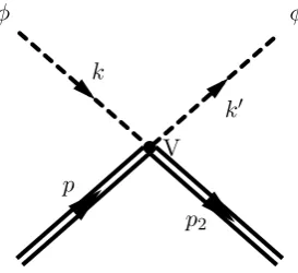
8. Constraints from Stellar Burning
p k
p2 k0
φ φ
[image:18.595.227.364.69.194.2]V
Figure 3: The disformal scalar scattering off a nucleon in the stellar medium.
horizontal branch stars all place constraints on the strength of the disformal coupling. An order of magnitude estimate of the constraints in [6] requiredM &30 GeV. In this section we consider the different production processes in turn in the following subsections, but begin with a calculation of the mean free path of a scalar in the stellar interior.
In what follows we will make a number of approximations in order to enable us to compute the energy loss rates analytically. Numerical simulations of the interior of stars would allow more precise bounds to be placed on the disformal scalar, this work is currently in progress [43].
8.1 The Scalar Mean Free Path
It is simplest to calculate the effects of scalar emission from stars if, once produced, the scalars escape from the star without further interaction. This happens provided the mean free path of the scalar due to the disformal interaction with fermions, shown in Figure 3, is larger than the size of the star.
The mean free path is related to the reaction rate between disformal scalars and nu-cleons in the stellar interior as
`= 1
Γ , (8.1)
where
Γ =
Z /
d3pfpσ , (8.2)
σ= 1
2Ep2Ek|~vk−~vp| Z /
d3k0
2Ek0 / d3p2
2E2
/
δ(4)(k0+p2−k−p)|M|2 , (8.3)
and the difference of velocities is close to unity as the scalars are massless and the fermions are non-relativistic. The matrix element is simply
M= ¯u(p2)V u(p), (8.4)
whereV is the four point vertex from the disformal coupling given in Equation (2.15). In the non-relativistic approximation whereE2 ∼Ep ∼mψ, the cross section is
σ = m
2
ψEk4
and this gives rise to a reaction rate
Γ =nψ m 2 ψE4k
16πM8 , (8.6)
where nψ is the number density of the fermionψ. Finally the mean free path is found to be:
`= 16π(Z+N) Z
M8 ρT4m
p
, (8.7)
whereZ is the atomic number of the dominant atoms in the star and N is the number of neutrons. In the Sun, where hydrogen burns predominantly we have Z = 1, N = 0 while on the Horizontal Branch (HB) where Helium burns we haveZ = 2, N = 2. The mass of the proton is mp and we have assumed that the highest energy available to the scalars is of the order of the stellar temperatureT.
To estimate the mean free path for the different stars we will consider in the following, we take the most stringent lower bounds on M obtained in the previous section from considerations of particle physics M > 120 GeV. We then find that in the Sun (ρ ∼ 150 g.cm−3 and T ∼1.5×10⁷ K)
`&2×1038 km, (8.8) where the solar radius is R ∼ 7×10⁵ km. For stars on the horizontal branch (ρ ∼ 104 g.cm−3 and T ∼1×10⁸ K)
`HB &4×1033 km, (8.9) where a typical radius isR∼3×10⁷ km. Finally for supernovae
`SN &109 km, (8.10) larger than the progenitor solar radius. Hence the stars are transparent to scalars inter-acting with matter via the disformal coupling.
8.2 Unitarity Constraints
All of the calculations that we will study in this section are perturbative and must preserve the unitarity of the underlying field theory. In the non-relativistic approximation which is valid in all the environments from main sequence stars to supernovae, the matrix elements for the scattering a scalar off a fermion f φ→f φinvolving the disformal coupling is given by
M ∼ m 2 fE2
M4 (8.11)
whereE is the energy of the incoming scalar. Unitarity imposes thatM.16π where the typical energy of scalars created in the stellar medium is E ∼T, the temperature of the star. We must therefore require that
M &
mfT 4√π
1/2
p p2 k
k0
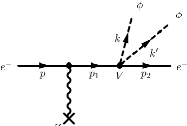
p1 e−
Ze
e− φ
φ
[image:20.595.203.387.72.196.2]V
Figure 4: Bremsstrahlung of disformal scalars by an electron scattering off a nucleus.
p p1˜
k
k0
p2 e−
Ze
e−
φ φ
˜ V
Figure 5: Bremsstrahlung of disformal scalars by an electron scattering off a nucleus.
for perturbative unitarity to stand. This constraint is easily satisfied in main sequence stars such as the sun where T ∼1.3 keV andmf =mp, we find
M &31 keV. (8.13)
For stars on the horizontal branch where THB ∼8.6 keV, we find
M &1 MeV. (8.14)
Finally in supernovae whereT ∼30 MeV we have
M &63 MeV. (8.15)
All these bounds are much weaker than the ones we will now derive from stellar burning rates.
8.3 Bremsstrahlung
The bremsstrahlung process of scalar production is shown in Figures4and5. We consider the emission of two scalars from the initial or final electrons interacting with the nucleus of an atom withZ protons. The matrix element corresponding to this process can be written as
MT =M+ ˜M, (8.16)
where M describes scalar radiation from the final state electron, and ˜M from the initial state electron. We have
M= Ze
2
|~p1−p|~2+m2D
1
p2 1+m2e
¯
[image:20.595.207.388.225.340.2]where the disformal vertex,V, is given in Equation (2.15).
In the plasma where the electrons evolve, the photons are not massless and have a mass given by the Debye mass
mD =
P iqi2ni
T
1/2
=
4π
1 +NZ+2Z
αρ
mpT
1/2
, (8.18)
where the charged particles are the electrons with charge−eand the nuclei with chargeZe. The densities arene =Znnuclei and (N+Z)ne= mρp whereρ is the plasma density,mp the proton mass, andN the number of neutrons in the nuclei. Numerically, we find that in the Sun we havemD ≈9.5 keV and in horizontal branch stars we havemD ≈0.03 MeV. This
is larger than the energy scale associated with the temperatures of the stars, respectively
T≈1.3 keV andTHB ≈8×10⁻³ MeV.
We define ˜V where we exchange p1 → p˜1 in Equation (2.15) and ˜M where p1 → p˜1 and V →V˜ in Equation (8.17). This gives
˜
M= Ze
2
|˜
~p1−p~2|2+m2D 1 ˜
p2 1+m2e
¯
u(p2)γ0(ip/˜1+mN) ˜V u(p). (8.19)
The emission rate of disformal scalars from a star, Γ, is given by the integral
Γ = 1 2EvE
Z d/3k
2Ek / d3k0
2Ek0 / d3p2
2E2
/
δ(E−E2−Ek−Ek0)(Ek+Ek0)|MT|2 , (8.20)
where the velocity is vE = m|~p|
e, and |MT|
2 is the squared matrix element averaged over
spins. The averaged energy loss rate per unit mass is given by
= nnuclei
ρ Z
/
d3pfpΓ, (8.21)
wherefp is the thermal distribution of the initial electron which is non relativistic
fp = ρ 2mp
2π meT
3/2 e− p~
2
2meT . (8.22)
In the non-relativistic limit, the squared matrix element becomes
|MT|2 = 64Z2e4m6e M8
Ek2Ek02
(p21+m2
e)2(|p~1−~p|2+m2D)2
. (8.23)
Inserting 1 =Rd/4p1/δ(p1−p2−k−k0) we find that
Γ = 1 2EvE
Z / d3p1
/ d3p2
2E2
θ(−(p1−p2)2) 8π h|MT|
2i (8.24)
= 1
2EvE Z
/ d3p1
/ d3p2
2E2
θ(−q2) 10π
(E−E2)P(q0, ~q) (p2
1+m2e)2(|p~1−~p|2+m2D)2
whereq =p1−p2 and the polynominal P is given by
P(q0, ~q) = a 3dq
2
0−
2b+ 4c 3d q
2
0q2+q4, (8.26)
where q2 = −q20+~q2 and we have defined the coefficients a= 301, b =−601, c = 601, d= 1
15×16 following the notation of Itzykson and Zuber [29]. Performing thep~2, integral first
we find that the constraint (p1−p2)2≤0 reduces to
|~q| ≤ |p~
2−p~
12|
2me , (8.27)
and therefore
Γ = 1
2EvE
Z2e4m5 e 35π3
Z
/ d3p1
|~
p2−p1~2| 2me
8
(p2
1+m2e)2(|p~1−p~|2+m2D)2
. (8.28)
The domain of the p~1 integration is|p~1| ≤
|~p2−p1~2|
2me implying that |p~1| ≤ ~ p2
2me, therefore we find that
Γ = 4Z
2α2me
105πM8|p~|
~ p2 2me
9
m2e (~p2+m2
D)2
. (8.29)
The rate per unit mass is now given by explicit integration
= Z
2α2me
210π3Am p ρ T M 8 1 (2πmeT)3/2g
m2D 2meT
, (8.30)
whereA=N +Z and
g(x) =
Z ∞
0
du u
9e−u
(u+x)2 . (8.31)
For the Sun, the energy loss rate per unit mass must be.0.1 erg/s.g [44]. Taking, as before, the temperature of the Sun to beT ∼1.5 107 K and the densityρ∼150 g/cm3, we find that this implies
M &39 MeV. (8.32)
For stars on the horizontal branch, we have T ∼108 K,ρ∼104 g/cm3 and the energy loss rate due to scalars is constrained to be HB .10 erg/s.g. We find that this requires
MHB &173 MeV. (8.33)
8.4 Compton Scattering
A pair of scalars can also be produced by Compton scattering between one fermion and one photon, see Figure6. The emission rate is given by
Γ = 1
2Ep2EK|~vE −~vK| Z /
d3k
2Ek / d3k0
2Ek0 / d3p2
2E2
/
p p2 k
k0 p1
e− e−
γ φ
φ
[image:23.595.204.387.67.154.2]˜ V
Figure 6: Compton process for production of disformal scalars.
where again the velocity difference is|~vE−~vK| ∼1 as the photons are relativistic and the fermions non-relativistic, and|MT|2is the squared matrix element averaged over spins and polarizations. The averaged energy loss rate per unit mass is given by
= 1 ρ
Z
/
d3p/d3KfpfKΓ, (8.35)
wherefp is the thermal distribution of the initial fermion which is non relativistic, and fK the photon distribution function. The matrix element is given by
M= e
p2
1+m2ψ
¯
u(p2)V(i /p1+mψ)γµµu(p), (8.36)
whereµ is the photon polarization vector normalized such that
X
µν =ηµν , (8.37)
and the sum is over the two polarizations. We have that
|MT|2 =− e 2
2(p2
1+m2ψ)2
Tr((p2/ −imψ)V(i /p1+mψ)(/p+ 2imψ)(i /p1+me)V). (8.38)
The initial and final fermions are non-relativistic while the photon spectrum is peaked around a temperature T that is less than the fermion mass. In this approximation we find that
|MT|2= 2e
2m6
ψ (p21+m2ψ)2
Ek2Ek02
M8 , (8.39)
and the emission rate becomes
Γ =
Z
/
d3qθ(−q2) e
2m4
ψ 32π(p2
1+m2ψ)2
hEk2Ek02i
M8 , (8.40)
whereq=p1−p2. We have used the approximationEk+Ek0 ∼EK. The condition q2≤0 implies that
(q0)2≥~q2 = (p~1−p~2)2, (8.41)
wherep1=p+K =p2+k+k0. UsinghEk2Ek02i=aq40−(2b+ 4c)q20~q2+ 3d(~q)2 , andX=|~q|, we have
Z
/
d3qθ(−q2)hEk2Ek02i= 24dq 7 0
k
k0 γ
Ze
φ φ
[image:24.595.211.383.69.198.2]V
Figure 7: The Primakov process for producing disformal scalars.
whered= 1/15×16 and with q0∼EK. Now using
p21+m2ψ ∼ −2mψEK , (8.43)
we find that
Γ = 3d 28(2π)3
e2m2ψEK5
M8 . (8.44)
The emission rate is maximal for protons, hence we deduce the energy loss rate due to scalars produced by Compton scattering to be
= 3dh 8π(2π)3
αZmp (Z+N)
T M
8
, (8.45)
where
h=
Z ∞
0
u7du
eu−1 . (8.46)
We find that the emission rate is smaller than that allowed for stars on the horizontal branch when
M &811 MeV, (8.47)
and for the Sun when
M &236 MeV. (8.48)
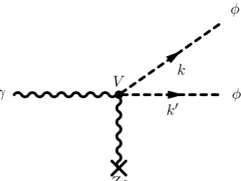
8.5 Primakov Process
We now consider the coupling between photons and the scalar field due to the disformal term
1
M4∂µφ∂νφ
FνaFaν− η µν
4 F 2
, (8.49)
which can lead to productions of scalars in the interior of a star due to the Primakov process shown in Figure 7. The coupling in Equation (8.49) leads to a four particle interaction vertex in the Feynman diagram expansion of perturbation theory:
Vγ = 1
M4 (p.k)(p 0
.k0)(.0)−(p.k)(k0.0)(p0.)−(p.0)(k.)(p0.0)
+(p.p0)(k.)(k0.0)− (k.k
0)
2 [(. 0
)(p.p0)−(p0.)(p.0)]
whereand 0 are the polarization vectors of the incoming photons of momenta (p, p0) and the scalars have momenta (k, k0).
The Primakov effect occurs when an incoming photon interacts with the electric field of a nucleus:
Ze ~
p02+m2 D
0µ, (8.51)
where0µ= (1,0,0,0). To simplify the calculations, we take the real and external photons to have transverse polarizations where 0 = 0. As a result the vertex becomes
Vγ = 1 M4
Ek0 (p.p0)(k.)−(p.k)(p0.)+Ep
(k.k0) 2 (p
0.)−(k.)(p0.k0)
. (8.52)
The matrix element is simply
M= Ze
~
p02+m2 D
Vγ. (8.53)
The emission rate is given by
Γ = 1 2Ep
Z /
d3k 2Ek
/ d3k0
2Ek0 /δ(Ek+E 0
k−Ep)(Ek+E 0
k)|MT|2 , (8.54)
where |MT|2 is the square of the matrix element averaged over the polarizations of the incoming photon. The energy loss rate is given by
γ= nnuclei
ρ
Z
/
d3pfpΓ. (8.55)
The calculation can be simplified by introducing the four-vector p0 = (0, ~p0) and inserting 1 =R /d3p0/δ(3)(p~0+~p−~k−k~0) in Γ so that it becomes
Γ = 1 32π
Z
/
d3p0θ(−q2) Z 2e2
(~p02+m2 D)2
hTr(Vγ2)i, (8.56)
where the expectation valueh.iwas defined in Equation (4.8), andq =p+p0. We find that
Tr(Vγ2) = 1
M8
Ek02 p02(p.k)2−2(p.k)(p.p0)k.p0+E2p
(k.k0)2 4 p
02−(k.k0
)(p0.k0)(p0.k)
+2EpEk0
k.k0
2 ((p.p
0)(k.p0)−p02(p.k)) + (p.k)(p0.k0)(p0.k)
. (8.57)
The domain of integration is defined by q2 ≤0, or equivalently ~p02+ 2~p.~p0 ≤0. Defining the angle θ = (~p, ~p0) between p~ and ~p0, and X = cosθ, the integration can be performed overp0 =p~p2 such thatp0 ≤ −2XE
p and then overX where−1≤X≤0. In addition we
approximate p~02+m2D ∼m2D which is justified as long asT .mD valid for the Sun and horizontal branch stars. After an extremely lengthy calculation to obtainhTr(Vγ2)iand the phase space integral over p~0, we find that
Γ = U Z 2e2
16(2π)3
Ep11 m4
DM8
K
p p2
k k0
π
K2 p1
φ
φ
V
Figure 8: Production of disformal scalars by pion exchange.
K
p p˜1
k
k0
π
K2 p2
φ φ
˜ V
Figure 9: Production of disformal scalars by pion exchange.
whereU = 9913314175. The loss rate becomes
γ=
U hZ2α 4π(2π)3
T14
mpm4DM8 , (8.59)
whereh=R∞
0 dx
x13 ex−1.
Bounding the energy loss rate due to Primakov production of disformal scalars in horizontal branch stars yields
M &346 MeV, (8.60)
and the corresponding bound from the Sun is
M &40 MeV. (8.61)
8.6 Pion Exchange
The interiors of supernovae differ substantially from the interiors of main sequence and horizontal branch stars. The dominant process for producing disformal scalars becomes the creation of two scalars with the exchange of one pion between two nuclei. The diagrams are depicted in Figures8 and9. As before we define the emission rate
Γ = 1
2Ep2EKvp
Z /d3k
2Ek / d3k0
2Ek0 / d3p2
2E2
/ d3K2 2EK2
/
δ4(p2+K2+k+k0−p−K)(Ek+Ek0)|NT|2, (8.62)
and the rate per unit mass
= 1
ρ Z
/
Fortunately, in the non-relativistic limit, the rate per unit mass from the pion exchange can be related to the previous bremsstrahlung calculation. Indeed the pion propagators reduce to 1
(~k+k~0)2+m2 π
and the nucleon propagator is simply 1
(~k+k~0)2 implying that one can factorize the propagators and write
NT =
A2g2πN N
((p1−p)2+mπ2)(p21+m2N)
[N1+N2+N3+N4], (8.64)
where the number of nucleons per nucleus is A =Z+N. We consider that the nucleons interact coherently, and we have defined
N1 = (¯u(p2)V(i /p1+mN)γ0u(p))¯u(K2)u(K),
N2 = (¯u(p2)(ip˜/1+mN) ˜V γ0u(p))¯u(K2)u(K),
N3 = (¯u(K2)W(i /K1+mN)γ0u(K))¯u(p2)u(p),
N4 = (¯u(K2)(iK˜/1+mN) ˜W γ0u(K))¯u(p2)u(p).
(8.65)
The scalar-pion vertices that we label W and ˜W follow the same pattern as V and ˜V in Section8.3 with thep momenta replaced byK’s. We find that
|NT|2 = 2 9A4g4
πN Nm8N M8
Ek2Ek02
(p21+m2N)2(|p~
1−~p|2+m2π)2
, (8.66)
from which we can directly obtain that
Γ = 4A 4α2
πmN
210πM8|~p|
~ p2
2mN 9
m2N
(~p2+m2
π)2
, (8.67)
where απ = g2
πN N
4π ∼ 13.5. Using R
/
d3KfK = n2N = 2mρp the total number of nucleons
divided by 2 (where we take all the nucleons to have the proton mass), we find that
= A
4α2
π
105π3ρ
T M
8
1 (2πmNT)3/2
g
m2
π
2mNT
. (8.68)
Observations of supernova SN1987A, constrain the energy loss due to any new physics to be SN .1019erg/s.g. Taking the supernova to have a temperature ofT = 30 MeV and
a densityρ∼3×10¹⁴ g/cm3, we find that
M &92 GeV. (8.69)
Source of bound Lower bound on M in GeV Environment Discussed in Section
Unitarity at the LHC 30 Lab. vac. 3
CMS mono-lepton 120 Lab. vac. 3
CMS mono-photon 490 Lab. vac. 3
Torsion Balance 7×10⁻⁵ Lab. vac. 4.1
Casimir effect 0.1 Lab. vac. 5.1
Hydrogen spectroscopy 0.2 Lab. vac. 6
Neutron scattering 0.03 Lab. vac. 7
Bremsstrahlung 4×10⁻² Sun 8.3
0.18 Horizontal Branch 8.3
Compton Scattering 0.24 Sun 8.4
0.81 Horizontal Branch 8.4
Primakov 4×10⁻² Sun 8.5
0.35 Horizontal Branch 8.5
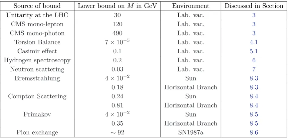
[image:28.595.83.560.82.310.2]Pion exchange ∼92 SN1987a 8.6
Table 1: Summary of the constraints on the disformal coupling scaleM. Lab. vac. means the constraint derives from a laboratory vacuum on Earth. Horizontal branch means the constraint derives from observations of horizontal branch stars, and similarly for constraints labelled Sun.
9. Summary and Conclusions
9.1 Summary of Constraints
In Table1we summarize the constraints on disformal couplings derived in this paper, and give a reference to the section in which each constraint is derived. The most constraining observations are the null results of mono-photon searches for beyond the Standard Model physics performed by the CMS collaboration. We present each constraint with a comment on the environment it is derived in, as in some theories with disformal couplings, such as the Galileon [45], the coupling scale can be renormalized by an environmentally dependent factor. We hope this will allow the reader to apply these results to their preferred theory with a disformal coupling.
9.2 Conclusion
force that could have consequences in atomic physics. The disformal interaction also plays a role in the heart of stellar objects where the disformal coupling opens up new channels for their burning rates. We have calculated the energy emission rates due to the disformal interaction in stars on the main sequence and the horizontal branch, and found stringent bounds on the disformal coupling strength.
The astrophysical effects following our new calculation on the disformal burning rates of stars can be applied to study the disformal effects on the Hertzsprung-Russell diagram of stellar structures; this is under study. In another publication, we also explore in further detail the applications of the disformal coupling to atomic physics.
Acknowledgements
We would like to thank Christoph Englert for discussions about collider constraints on disformal scalars. We would also like to thank Jose Cembranos and Jeremy Neveu for helpful communications. C.B. is supported by a Royal Society University Research Fellow-ship. P.B. acknowledges partial support from the European Union FP7 ITN INVISIBLES (Marie Curie Actions, PITN- GA-2011- 289442) and from the Agence Nationale de la Recherche under contract ANR 2010 BLANC 0413 01.
References
[1] E. J. Copeland, M. Sami and S. Tsujikawa, Int. J. Mod. Phys. D15(2006) 1753 [hep-th/0603057].
[2] T. Clifton, P. G. Ferreira, A. Padilla and C. Skordis, Phys. Rept.513(2012) 1 [arXiv:1106.2476 [astro-ph.CO]].
[3] E. G. Adelberger, B. R. Heckel and A. E. Nelson, Ann. Rev. Nucl. Part. Sci.53 (2003) 77 [hep-ph/0307284].
[4] J. D. Bekenstein, Phys. Rev. D48(1993) 3641 [gr-qc/9211017].
[5] T. Kugo and K. Yoshioka, Nucl. Phys. B594(2001) 301 [hep-ph/9912496].
[6] N. Kaloper, Phys. Lett. B583(2004) 1 [hep-ph/0312002].
[7] P. Brax, C. Burrage and A. -C. Davis, JCAP1210 (2012) 016 [arXiv:1206.1809 [hep-th]].
[8] M. Wyman, Phys. Rev. Lett.106(2011) 201102 [arXiv:1101.1295 [astro-ph.CO]].
[9] S. Sjors and E. Mortsell, JHEP1302(2013) 080 [arXiv:1111.5961 [gr-qc]].
[10] J. Neveu, V. Ruhlmann-Kleider, P. Astier, M. Besanon, A. Conley, J. Guy, A. Mller and N. Palanque-Delabrouilleet al., arXiv:1403.0854 [gr-qc].
[11] C. van de Bruck, J. Morrice and S. Vu, Phys. Rev. Lett. 111(2013) 161302 [arXiv:1303.1773 [astro-ph.CO]].
[12] P. Brax, C. Burrage, A. -C. Davis and G. Gubitosi, JCAP1311 (2013) 001 [arXiv:1306.4168 [astro-ph.CO]].
[14] T. S. Koivisto, D. F. Mota and M. Zumalacarregui, Phys. Rev. Lett.109(2012) 241102 [arXiv:1205.3167 [astro-ph.CO]].
[15] D. Bettoni, V. Pettorino, S. Liberati and C. Baccigalupi, JCAP 1207(2012) 027 [arXiv:1203.5735 [astro-ph.CO]].
[16] C. de Rham and A. J. Tolley, JCAP1005 (2010) 015 [arXiv:1003.5917 [hep-th]].
[17] T. Koivisto, D. Wills and I. Zavala, arXiv:1312.2597 [hep-th].
[18] J. Alcaraz, J. A. R. Cembranos, A. Dobado and A. L. Maroto, Phys. Rev. D67(2003) 075010 [hep-ph/0212269].
[19] J. A. R. Cembranos, A. Dobado and A. L. Maroto, Phys. Rev. D70 (2004) 096001 [hep-ph/0405286].
[20] C. de Rham, G. Gabadadze and A. J. Tolley, Phys. Rev. Lett.106(2011) 231101 [arXiv:1011.1232 [hep-th]].
[21] C. de Rham and G. Gabadadze, Phys. Rev. D82(2010) 044020 [arXiv:1007.0443 [hep-th]].
[22] P. Brax, Phys. Lett. B712(2012) 155 [arXiv:1202.0740 [hep-ph]].
[23] E. Babichev, V. Mukhanov and A. Vikman, JHEP0802(2008) 101 [arXiv:0708.0561 [hep-th]].
[24] C. Burrage, C. de Rham, L. Heisenberg and A. J. Tolley, JCAP1207 (2012) 004 [arXiv:1111.5549 [hep-th]].
[25] CMS Collaboration [CMS Collaboration], pp collision events at center-of-mass energy of 8 TeV ,” CMS-PAS-EXO-13-004.
[26] Y. Bai and T. M. P. Tait, Phys. Lett. B723(2013) 384 [arXiv:1208.4361 [hep-ph]].
[27] J. A. R. Cembranos, R. L. Delgado and A. Dobado, Phys. Rev. D88 (2013) 075021 [arXiv:1306.4900 [hep-ph]].
[28] CMS Collaboration, CMS-PAS-EXO-12-047 .
[29] C. Itzykson and J. B. Zuber, New York, Usa: Mcgraw-hill (1980) 705 P.(International Series In Pure and Applied Physics)
[30] E. G. Adelberger, J. H. Gundlach, B. R. Heckel, S. Hoedl, S. Schlamminger, Progress in Particle and Nuclear Physics,62, (2009), 102-134,
[http://dx.doi.org/10.1016/j.ppnp.2008.08.002].
[31] R. L. Jaffe, Phys. Rev. D72(2005) 021301 [hep-th/0503158].
[32] S. K. Lamoreaux, Phys. Rev. Lett.78(1997) 5 [Erratum-ibid.81 (1998) 5475].
[33] T. Jenke, G. Cronenberg, J. Burgdorfer, L. A. Chizhova, P. Geltenbort, A. N. Ivanov, T. Lauer and T. Linset al., Phys. Rev. Lett.112(2014) 151105 [arXiv:1404.4099 [gr-qc]].
[34] P. Brax and G. Pignol, Phys. Rev. Lett. 107(2011) 111301 [arXiv:1105.3420 [hep-ph]].
[35] P. Brax and C. Burrage, Phys. Rev. D83(2011) 035020 [arXiv:1010.5108 [hep-ph]].
[36] R. Pohl, R. Gilman, G. A. Miller and K. Pachucki, Ann. Rev. Nucl. Part. Sci.63(2013) 175 [arXiv:1301.0905 [physics.atom-ph]].
[38] V. V. Nesvizhevsky, G. Pignol and K. V. Protasov, arXiv:0705.4478 [nucl-ex].
[39] C. Schwob, L. Jozefowski, B. de Beauvoir, L. Hilico, F. Nez, L. Julien, F. Biraben and O. Acefet al., Phys. Rev. Lett.82(1999) 4960.
[40] J. Jaeckel and S. Roy, Phys. Rev. D82(2010) 125020 [arXiv:1008.3536 [hep-ph]].
[41] P. J. Mohr, B. N. Taylor and D. B. Newell, Rev. Mod. Phys.84(2012) 1527 [arXiv:1203.5425 [physics.atom-ph]].
[42] P. Brax, C. Burrage, To appear.
[43] P. Brax, C. Burrage, J. Sakstein, To appear.
[44] G. G. Raffelt, Chicago, USA: Univ. Pr. (1996) 664 p
[45] A. Nicolis, R. Rattazzi and E. Trincherini, Phys. Rev. D79(2009) 064036 [arXiv:0811.2197 [hep-th]].