Pattern formation with a conservation law

arXiv:nlin.PS/0006002 1 Jun 2000

P. C. Matthews and S. M. Cox

School of Mathematical Sciences, University of Nottingham, University Park, Nottingham NG7 2RD, UK

Abstract. Pattern formation in systems with a conserved quantity is considered by studying the appropriate amplitude equations. The conservation law leads to a large-scale neutral mode that must be included in the asymptotic analysis for pattern formation near onset. Near a stationary bifurcation, the usual Ginzburg–Landau equation for the amplitude of the pattern is then coupled to an equation for the large-scale mode. These amplitude equations show that for certain parameters all roll-type solutions are unstable. This new instability differs from the Eckhaus instability in that it is amplitude-driven and is supercritical. Beyond the stability boundary, there exist stable stationary solutions in the form of strongly modulated patterns. The envelope of these modulations is calculated in terms of Jacobi elliptic functions and, away from the onset of modulation, is closely approximated by a sech profile. Numerical simulations indicate that as the modulation becomes more pronounced, the envelope broadens. A number of applications are considered, including convection with fixed-flux boundaries and convection in a magnetic field, resulting in new instabilities for these systems.

PACS numbers: 47.54.+r, 02.30.Jr, 05.45.-a

1. Introduction

The mathematical theory of pattern formation has a wide range of applications. In the field of fluid mechanics, the most widely studied example is Rayleigh–B´enard convection and its variants, but there are many other examples such as Taylor–Couette flow and solidification of alloys. Pattern-forming systems can also be found in many chemical and biological systems (see the review by Cross and Hohenberg 1993).

In this paper we consider pattern formation in one space dimension in systems sufficiently large to allow a large-scale modulation of the pattern. It is assumed that the system has some reflection symmetry, that the onset of instability is stationary, and that the onset of pattern formation occurs with a non-zero wavenumber. In this case, the equation governing the modulation of the small-amplitude pattern is in general the real Ginzburg–Landau equation. This well known result has recently been given rigorously by Melbourne (1999). The behaviour of the real Ginzburg–Landau equation is straightforward: a regular periodic pattern is stable provided its wavenumber lies within the Eckhaus band (Eckhaus 1965); patterns outside this band are unstable, and the instability is subcritical (Fauve 1987, Tuckerman and Barkley 1990). Physically, patterns in which the wavenumber is either too large or too small adjust to a different wavenumber by adding or losing waves.

1993, p. 883). To be specific, we suppose that this conservation law may be written in the form

∂w ∂t +

∂

∂xf(w) = 0,

with appropriate boundary conditions, from which it follows thatwis conserved, that is,

d dt

Z

wdx= 0,

where the integral is taken over the entire spatial domain. The conservation law leads to a neutral large-scale mode, which must be included in the dynamics if a correct description of the behaviour near onset is to be obtained.

The resulting behaviour depends on how the reflection symmetry acts on the large-scale mode. The case in which the large-scale mode changes sign upon reflection arises when the system has Galilean invariance (Coullet and Fauve 1985). This case was studied by Matthews and Cox (1999), who showed that all steady patterns are unstable, with the instability growing more rapidly than the rate of formation of the pattern. As a consequence, a highly disordered state is found, even near onset.

In this paper we study the case where the large-scale mode does not change sign under reflection. Physically, this corresponds to the mode representing a density rather than a flow. Similar problems have been considered by Riecke (1992a, 1992b, 1996) and Herrero and Riecke (1995) for convection in binary mixtures, but in this case the bifurcation is oscillatory and asymptotically self-consistent amplitude equations were not obtained.

Experiments demonstrating the effects of coupling between short-scale pattern modes and large-scale mean flows have been carried out in a variety of flows. In surface tension-driven convection, VanHook et al. (1995, 1997) have shown how the presence of a large-scale surface-deformational mode can lead to dry spots and high spots. In a two-layer viscous shear flow (Barthelet and Charru 1998, Charru and Barthelet 1999), finite-amplitude interfacial waves become unstable through coupling to a large-scale mode which may be traced back to conservation of mass of each fluid. In liquid crystals (Hidakaet al.1997), complicated spatio-temporal convection patterns are traced to the presence of a large-scale mode arising in the degeneracy of the system.

The paper is organised as follows. In _§ 2 we derive the governing amplitude equations by symmetry and scaling arguments and then, in _§ 3, analyse their properties. We consider the stability of small-amplitude solutions, and the behaviour of fully nonlinear solutions of the amplitude equations, in particular localised states. In _§ 4 we illustrate how the insights we have gained apply to a model partial differential equation (PDE), through numerical simulation. We also demonstrate how the behaviour of the full PDE diverges from that predicted by the leading-order amplitude equations, as the parameters are varied, and analyse this divergence in_§ 5. We then describe, in _§ 6, three physical examples in which our amplitude equations arise. In_§ 7 we summarise our results.

2. Derivation of mean-mode and pattern-mode equations

from symmetry considerations, while in § 2.2 a model PDE is introduced and the amplitude equations are derived by asymptotic expansions near the onset of pattern formation.

2.1. Derivation of equations from symmetry

Consider a PDE or system of PDEs with a conserved quantity and a basic zero state. If a quantityw(x, t) is conserved, it must be possible to write∂w/∂tas the divergence of a flux. It follows that when the expression for ∂w/∂t is linearised, there can be no terms linear inwexcept those involvingx-derivatives. If we assume, furthermore, that the system possesses the reflection symmetry

x_{→ −}x, w_→w (2.1)

then only even x-derivatives occur. Thus w is density-like (a velocity-like quantity would satisfy x → −x, w → −w instead; see Matthews and Cox (1999), Tribelsky and Velarde (1996)). On large spatial scales, the leading linear term is the second derivativewxx, sow(x, t) obeys the diffusion equation and the growth rateλof modes

with wavenumber k is proportional tok2. This indicates that large-scale modes are almost neutral, evolving on a long timescale, and must be included in the analysis of pattern formation.

Suppose that the system supports stationary patterns with a wavenumber k, which we take to be the critical wavenumber according to linear stability theory; we may set k = 1 with no loss of generality. Near the onset of pattern formation the appropriate ansatz is then

w(x, t)_∼A˜(X, T)eix_{+ ˜A}∗_{(X, T)e}−ix_{+ ˜B(X, T), (2.2)}

where X and T are rescaled forms of x and t, and ˜A and ˜B are small amplitudes. Note that the amplitude ˜Ais complex, withA∗denoting the complex conjugate ofA, but ˜B is real.

The amplitude equations for ˜A and ˜B can be written down by imposing the symmetries of translation inx

˜

A_→Ae˜ iχ, B˜_→B˜ (2.3)

and reflection

X_{→ −}X, A˜_→A˜∗, B˜_→B.˜ (2.4)

In the absence of the large-scale mode ˜B, ˜Aobeys the real Ginzburg–Landau equation. Coupling terms in this equation must include ˜A because of (2.3), so the leading coupling term in the ˜A equation that is consistent with the symmetries is ˜AB˜. The coefficient of this term is forced to be real by (2.4). In the absence of coupling terms, the equation for ˜Bis the diffusion equation, and (2.3) forces coupling terms to involve equal numbers of ˜Aand ˜A∗_{terms. Since ˜B is conserved, all terms in the ˜B equation} involve derivatives. The leading coupling term in the ˜B equation that is consistent with (2.4) is therefore (_|A˜_|2₎

XX.

These considerations give rise to amplitude equations of consistent asymptotic order if we introduce a small parameter such that ˜A = A, ˜B = 2_{B, X = x,}

T =2_{t. Furthermore, we take the system to be a distance ofO(}2_{) from the marginal} surface in parameter space. With these scalings, the amplitude equations truncated to leading order are then

AT =A+AXX−A|A|2−AB, (2.5)

-0.2 -0.1 0 0.1 0.2

0 0.2 0.4 0.6 0.8 1 1.2 1.4

λ

k

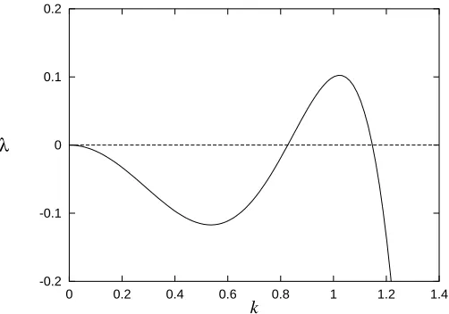
Figure 1. The growth rate λ of the linear modes of (2.7) as a function of wavenumberk, withr= 0.1.

where we have assumed that, in the absence ofB, the bifurcation of the pattern mode is supercritical. All coefficients in (2.5) have been set to unity by rescalingT,X,Aand

B. There are two coefficients,σandµ, in (2.6) that cannot be removed by rescaling. We impose the conditionσ >0 to ensure that the long-wavelength modes are weakly damped in the absence of A, but µ may have either sign. Equations analogous to (2.5)–(2.6) have previously been derived in the context of the secondary stability of cellular patterns (Coullet and Iooss 1990).

2.2. Derivation of equations from a model PDE

Consider the PDE

∂w ∂t =−

∂2

∂x2 "

rw₋

1 + ∂

2

∂x2 2

w₋sw2 −w3

#

, (2.7)

where the terms inside the brackets are just those of the much-studied Swift– Hohenberg equation (Swift and Hohenberg 1977) with a symmetry-breaking quadratic term (Sakaguchi and Brand 1996, Matthews 1998). This equation has the required properties of reflection symmetry and a conservation law forw(x, t).

The growth rateλof modes of wavenumberkin (2.7) is given by

λ=k2_(r

−(1₋k2₎2_{), (2.8)}

so for 0< r1 a narrow band of wavenumbers neark=kc= 1 is unstable (figure 1).

We now follow the standard asymptotic methods to describe the behaviour of (2.7) for smallr, by writing

r=2r2, T =2t, X=x. (2.9)

The appropriate asymptotic expansion forw(x, t) is then

w(x, t) =A(X, T)eix+A∗(X, T)e−ix+2B(X, T)

where the large-scale modeB has been introduced at order2_.

The expansion (2.10) is substituted into (2.7) and the system is then solved at successive orders of . At O(), (2.7) is automatically satisfied. At O(2_{), terms} involving e2ix _{appear, and from these we deduce that C = −sA}2_{/9. At O(}3_{), the} amplitude equation forAis deduced from the terms in eix_{. The equation forBfollows}

from the terms independent ofxatO(4_{). These equations are}

AT =r2A+ 4AXX−(3−2s2/9)|A|2A−2sAB, (2.11)

BT =BXX + 2s(|A|2)XX. (2.12)

The sign ofs is thus immaterial, and the bifurcation is supercritical ifs2_{<27/2. If} this condition is satisfied then (2.11) and (2.12) can be rescaled to give (2.5–2.6).

Although the system (2.5)–(2.6) is generic for pattern-forming systems with a conservation law, in fact a conservation law alone is not sufficient to yield these equations. Only the first of the two nonlinear terms in (2.7) generates the coupling term in (2.5), so if we sets= 0 there is no coupling and the dynamics is then governed by the Ginzburg–Landau equation alone. Furthermore, if the original PDE has the symmetryw_{→ −}wthen all nonlinear terms in (2.11) are cubic and again no coupling terms arise. This restriction will apply when we consider physical examples in_§ 6.

3. Analysis of the amplitude equations

In this section we analyse the steady solutions of the amplitude equations (2.5– 2.6). We begin by considering small-amplitude, periodic solutions (rolls). We then investigate the super/subcritical nature of the instability, and, beyond the point where rolls become unstable, we calculate fully nonlinear solutions of (2.5–2.6).

3.1. Stability of patterns

In this section we analyse the stability of periodic solutions in the form of rolls. Rolls with wavenumberkc+q correspond to solutions of (2.5–2.6) of the formA=a0eiqX

andB= 0, where the amplitudea0may be taken to be real and to satisfya20= 1−q2. To analyse the stability of these rolls, we set

A= (a0+a(X, T))eiqX, B=b(X, T), (3.1)

and linearise (2.5–2.6) in a and b. Upon setting a = V(T)eilX _+W∗_(T)e−ilX _and

b=U(T)eilX _+U∗_(T)e−ilX_{, we find}

˙

V = ₋(2q+l)lV ₋a2

0(V +W)−a0U, (3.2)

˙

W = ₋(₋2q+l)lW ₋a20(V +W)−a0U, (3.3) ˙

U = ₋σl2_U

−µa0l2(V +W). (3.4)

Solutions of (3.2–3.4) proportional to eλT _{have a growth rateλthat satisfies the cubic}

equation

λ3+ (2l2+σl2+ 2a02)λ2−l2(2µa20−2σa20−2a20−l2−2σl2+ 4q2)λ −l4_(2µa2

0−2σa20−σl2+ 4σq2) = 0. (3.5)

For modes withλreal, there is instability if

The most dangerous disturbance therefore arises in the limitl→0, and so the criterion for instability is

(µ−σ)a20+ 2σq2>0, (3.7)

or, equivalently,

µ(1−q2)> σ(1−3q2). (3.8) From (3.7) it is clear that all rolls are unstable if

µ > σ. (3.9)

If µ < σ then rolls of sufficiently small amplitude are unstable; the criterion for instability can be expressed in terms ofqas

q2>(σ₋µ)/(3σ₋µ). (3.10)

It is clear that when the coupling between the mean and pattern modes is removed (µ= 0), or more generally when _|σ/µ_| 1, the usual Eckhaus criterion q2_{>1/3 for} instability is recovered. In general, the band of stable rolls is narrowed ifµ >0 and widened ifµ <0.

Hopf bifurcations are also permitted in (3.5). We are able to make analytical progress in the small-llimit, where one solution of (3.5) is λ=₋2a2

0while the other two obey

λ2a20+λl2(a20(1 +σ−µ)−2q2) +l4(σ−µ−3q2σ+q2µ) = 0.(3.11) It follows that there is oscillatory instability ifq2_{>(1 +σ−µ)/(3 +σ−µ) provided} thatµσ−σ2_{−µ >0. From these conditions it can be deduced that a Hopf bifurcation} is possible only ifσ <1, µ <0 and q2 _{>1/3. There is a Takens–Bogdanov point (a} repeated zero eigenvalue) atq2_{= 1/(3}

−2σ) whenµ(σ₋1) =σ2_.

The stability results are summarised in figure 2. Note that the stationary bifurcation given by (3.10) depends only on the ratio µ/σ but this is not true for the Hopf bifurcation.

The mechanism of instability in (2.5–2.6) is rather different from that of the Eckhaus instability. Even rolls with q = 0 are unstable for µ > σ, and in this case the unstable mode has V = W so that a is real and the instability is amplitude-driven rather than phase-amplitude-driven. If there are regions where|A|2_{has a minimum, then,} according to (2.6),B grows in these regions ifµ >0. This leads to a positive value of

B which then reduces the size ofAfurther, through the coupling term in (2.5).

3.2. Nonlinear development of the instability

The results of_§3.1 show that forµ > σ, all periodic patterns in (2.5–2.6) are unstable. We now consider the nonlinear development of the instability, to determine whether the bifurcation is subcritical or supercritical. The Eckhaus instability, for example, is known to give rise to a subcritical bifurcation (Fauve 1987, Tuckerman and Barkley 1990).

For simplicity we consider the caseq= 0, corresponding to rolls with wavenumber

kc. These are the last rolls to become unstable as µ is increased. In this case the

stationary solution isA= 1,B= 0. WritingA= 1 +a(X, T),B=b(X, T), cf. (3.1), we find that the imaginary part ofa decays so that we may takea to be real. The nonlinear equations for the real-valued quantitiesaand bare then, from (2.5–2.6),

aT =−2a+aXX−3a2−a3−b−ab, (3.12)

0 0.2 0.4 0.6 0.8 1

-3 -2 -1 0 1 2 3

q

µ/σ

Unstable

Stable

Figure 2.Region of stable rolls in (2.5–2.6). The solid line shows the stationary bifurcation, which is valid for anyσ, and the dotted line shows the Hopf bifurcation forσ= 1/4. Forµ > σall rolls are unstable, while forµ < σthere is a band of stable rolls that widens asµis decreased. The usual Eckhaus result of stability forq2_<1

3 corresponds toµ= 0.

A weakly nonlinear analysis is now employed, by writing

µ=µ0+2µ2, T2=2T,

a=a1+2a2+O(3), b=b1+2b2+O(3),

where theai andbi are functions ofX andT2. By considering a single mode,

a1=a11(T2) coslX, b1=b11(T2) coslX,

we find that the terms of order in (3.12–3.13) give

b11+ (2 +l2)a11= 0 and µ0= (1 +l2/2)σ,

so the instability condition (3.9) is recovered for smalll. At O(2_{) we deduce that}

a2=a20+a22cos 2lX, b2=b22cos 2lX,

where

a20= (l2−1)a211/4, a22=a211/4 and b22=−(1 +l2/2)a211.

Applying the solvability condition atO(3_{) gives the equation for the evolution on the} slow timescaleT2:

(σl2+ 2 +l2)da11 dT2

= 2l2µ2a11+

σl4_(l2 −1)

2 a

3 11.

3.3. Nonuniform steady solutions

We now extend the analysis of the previous subsection to consider fully nonlinear stationary solutions of the amplitude equations (2.5)–(2.6). WritingA=Rexp iΘ, we find from the imaginary part of (2.5) that (R2_Θ

X)X = 0 and so ΘX = ΩR−2, where

Ω is constant. From (2.6) we find, for solutions periodic inX, that

B=µ0(hR2i −R2), (3.14)

where h· · ·i denotes a spatial average. In deriving (3.14), we have taken hBi = 0, which corresponds to an initial condition such that hwi= 0 (and hence hwi = 0 for all time). Any other initial value forhwiis equivalent tohwi= 0 under a rescaling of the parameters r and s in (2.7). From the real part of (2.5), it then follows that R

satisfies

0 = (1₋µ0_hR2_i)R+RXX −(1−µ0)R3−Ω2R−3. (3.15)

This equation may be integrated once, and is then more conveniently expressed in terms ofQ=R2:

Q02= 2(1₋µ0)Q3+ 4(µ0_hQ_{i −}1)Q2+ 4HQ₋4Ω2, (3.16)

where H is a constant of integration. The solution is readily determined in terms of the Weierstrass elliptic function P (Abramowitz and Stegun 1965, Whittaker and Watson 1962) to be

Q= 2

(1₋µ0₎P(X;g2, g3) +B, (3.17)

where

g2= −2(1−µ0)H+4₃(µ0hQi −1)2 (3.18)

g3= 23(1−µ0)(µ0hQi −1)H− 8

27(µ0hQi −1) 3_{+ (1}

−µ0)2Ω2 (3.19)

B = −2(µ0hQi −1)

3(1₋µ0₎ , (3.20)

andg2andg3are the usual parameters ofP. The amplitude and period of the solution are implicitly related through the appearance of the quantityhQiin (3.18)–(3.20).

Although (3.17) provides an exact solution, it requires specification ofµ0, H, Ω and the spatial period to permit analysis of its solutions. Rather more analytical progress is possible if we restrict attention to the invariant subspace in which A is real. We suppose that the solution has spatial periodL(note that, as a consequence,

L= 2nπfor some integern). Equations (2.5)–(2.6) become

0 =A+AXX −A3−AB, (3.21)

0 =BXX+µ0(A2)XX, (3.22)

where

µ0=µ/σ.

Integrating (3.22) twice and imposing periodicity gives the result

B+µ0A2=µ0hA2i, (3.23)

corresponding to (3.14). EliminatingBfrom (3.21) gives

0 = (1₋µ0_hA2

Before describing the periodic solutions of (3.21)–(3.22), it is instructive to consider a solution that is a good asymptotic approximation:

A=A0sech(cX), (3.25)

where µ0_hA2

i = 1 +c2 _{and µ}0_{= 1 + 2c}2_/A2

0. Note that the solution exists only for

µ0_{>1, which is consistent with the stability boundary (3.9) and the result from§3.2} that the bifurcation atµ0_{= 1 is supercritical. For large values ofcL, cLhA}2

i ∼2A2 0. Using this approximation for _hA_i, we obtain forcthe quadratic equation

c2

−4µ0c/L(µ0₋1) + 1 = 0,

which has real solutions only for

1< µ0< L/(L₋2), (3.26)

indicating that a saddle–node bifurcation occurs at µ0 _{= L/(L−2) and that for}

µ0 _{> L/(L−2) no such solution exists. At large amplitude the solution branch} approaches µ0 _{= 1 and the amplitude is given by A}

0 ∼ 4 √

2µ0_/L(µ0₋₁₎3/2_{. The} solution (3.25) is of particular significance because, as we shall see, it can be stable and is observed in the numerical simulations described in_§ 4.

Spatially periodic solutions of (3.24) can be written in terms of the Jacobi elliptic functions sn, cn and dn. In all that follows,m denotes the standard parameter of these functions (Whittaker and Watson 1962, Abramowitz and Stegun 1965), and we use the notation_{h· · ·i}as above, so that

hf(X)_{i ≡} 1 4K

Z 4K

0

f(X) dX,

whereK is the real quarter-period, given by

K(m) = Z π/2

0

dθ

(1−msin2θ)1/2.

3.3.1. dn When µ0_{>1, there exist solutions of (3.24) in the form}

A=A0 dncX, (3.27)

where

(2₋m)c2=A20µ0hdn 2

cX_{i −}1, 2c2=A02(µ0−1), cL= 2K. (3.28)

Given the parameterµ0_{and the lengthLof the domain, the three equations in (3.28)} serve to determine the three unknowns A0, c and m. However, the computation of solutions is more easily accomplished ifL, say, is fixed, whilemis varied in the range 0_≤m <1 to yield corresponding values of A0,candµ0_.

For smallm, the solution takes the form

A_∼(1 +1 4m)(1−

1 2msin

2_{(πX/L)), (3.29)}

indicating that these solutions branch from the uniform state A ≡1; the branching takes place at µ0= 1 + 2π2_/L2 _{(corresponding to m= 0). Furthermore, it is readily} shown from (3.28) that for smallm

µ0= 1 +2π 2

L2 +

π2 16L4(L

2

−4π2)m2+O(m3), (3.30)

1 2 3 4 5 6 7 8

1 1.02 1.04 1.06 1.08 1.1 1.12 1.14

A

µ/σ

Figure 3. The bifurcation diagram for (3.21)–(3.22) with periodic boundary conditions withL= 5π(solid line) andL= 10π(dashed line). Solutions take the form (3.27). The vertical axis shows the maximum value ofA.

Asmis increased from zero to unity, the corresponding values ofµ0_{increase to a} maximumµd (given approximately in (3.26) byµd∼L/(L−2)), and then decrease

monotonically so that

µ0∼1 + 4

ln(16/m1), (3.31)

asm→1−, where m1= 1−m. We have used the well known result that

K_∼ln(4/m1₁/2) (3.32)

in this limit. Thus a saddle–node bifurcation takes place atµ0=µd, and forµ0> µd

no solutions of the form (3.27) exist. Figure 3 shows the bifurcation diagram for dn-type solutions of (3.21)–(3.22) subject to periodic boundary conditions with L= 5π

and L = 10π. The saddle–node bifurcations occur at µd = 1.146 and µd = 1.068

respectively, in agreement with our approximation (3.26). Since the bifurcation is supercritical in each case, the lower branch of solutions is stable but the upper branch is unstable.

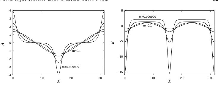
When m is small, the solution for A takes the form of small, almost sinusoidal perturbations to the uniform state A_≡1. Asm is increased, the peak ofAbecomes narrow and the trough broadens. Asm_→1−_{, the peak increases greatly in amplitude} and the solution takes the form

A_∼2K

3/2

L sech

2KX

L (3.33)

where µ0_{∼1 + 2/K, andK → ∞according to (3.32). In this limit, the solution for}

Athus takes the form of a single sech-type pulse as given by (3.25). The dn solutions are illustrated in figure 4.

These results indicate that forµd> µ0>1 a soliton-like solution exists to (2.5)–

(2.6). For µ0 > µd, numerical simulations of (2.5)–(2.6) indicate that the solution

-1 0 1 2 3 4

0 10 20 30

A

X

m=0.1

m=0.9999999

-5 -4 -3 -2 -1 0 1 2

0 10 20 30

B

X

m=0.1 m=0.9999999

Figure 4. Solution of (3.21) and (3.22) in terms of dn (3.27) form= 0.1, 0.5, 0.9, 0.999, 0.9999999 (corresponding toµ0_{= 1.0200, 1.0203, 1.0230, 1.0504, 1.0596).}

The spatial period isL= 31.4.

0 10 20 30 40

0 0.1 0.2 0.3 0.4 0.5 0.6 0.7 0.8 0.9 1

g(m)

m

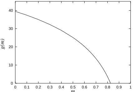
Figure 5. The functiong(m), defined in (3.36). The intercepts with the axes are given byg(0) = 4π2_andg(m

0) = 0, wherem0≈0.826115.

3.3.2. cn Whenµ0>1, solutions also exist in the form

A=A0 cncX, (3.34)

where

(2m₋1)c2=A02µ0hcn2cXi −1, 2mc2=A20(µ0−1), cL= 4K. (3.35)

When m is small, A ∼ √2(1−4π2/L2)1/2cos(2πX/L), and hence we require

L >2πfor the existence of this solution in this limit. Further analysis indicates that for general values ofma solution exists only when

L2> g(m)≡16K2[1 + 2m(hcn2cXi −1)]. (3.36)

The function g(m) is shown in figure 5. It is clear from (3.36) and figure 5 that if L > 2π the solution (3.34) exists for all m between zero and unity. If, on the other hand, L < 2π then solutions exist for mL < m < 1, where g(mL) = L2.

Regardless of the value ofL, these solutions exist form > m0≈0.826115. IfL >2π then as m is increased from zero, µ0 _{increases from unity to a maximum value µ}

c

-4 -3 -2 -1 0 1 2 3 4

0 10 20 30

A

X

m=0.1

m=0.999999

-15 -10 -5 0 5

0 10 20 30

B

X

m=0.1 m=0.999999

Figure 6. Solution of (3.21) and (3.22) in terms of cn (3.34) form= 0.1, 0.9, 0.999, 0.999999 (corresponding toµ0 _{= 1.004, 1.069, 1.128, 1.146). The spatial}

period isL= 31.4.

to (3.31) as m _→ 1−_{. If L < 2π then as m is increased from m}

L, µ0 decreases

monotonically from infinity, again according to (3.31) asm_→1−_.

Asmis increased, the peaks ofAbecome more pronounced, larger in amplitude and narrower, while the regions in whichAhas small amplitude become broader. In the limitm_→1−_{, the solution is approximately given by two sech-type pulses, one} positive and one negative; with an appropriate choice of origin inX, the solution for 0< X < Lsatisfies

A∼4K 3/2

L

sech4KX

L − sech

4K(X−L/2)

L

,

withK andmrelated through (3.32). The cn solutions are illustrated in figure 6.

3.3.3. sn The final type of solution that may be expressed in the form of Jacobi elliptic functions applies whenµ0<1, and is

A=A0 sncX, (3.37)

where

(1 +m)c2= 1−A20µ0hsn2cXi, 2mc2=A20(1−µ0), cL= 4K. (3.38) For small m, these solutions match with the cn solutions (allowing for an unimportant translation in X), with A _∼ √2(1₋4π2_/L2₎1/2_{sin(2πX/L). As this} expression indicates, the small-msolutions requireL >2π. In fact, for general values ofm, the lengthL of the domain must satisfy

L2_{> h(m)}

≡16K2_{[1 +m}

−2m_hsn2_cX

i]. (3.39)

The function h(m) is monotonic increasing, with h(0) = 4π2 _{and h(m) → ∞ as}

m_→1−_{. Thus solutions of the form (3.37) do not exist ifL <2π; ifL >2π, solutions} exist for 0< m < mL, whereh(mL) =L2. As mincreases towards mL,µ0 decreases

monotonically to_−∞, the peaks and troughs inAbecoming broader. Provided Lis large, the profile nearX = 0 is approximately a front of the form

A_∼tanh4KX

L

asm→m−L, the front near X =L/2 being given by symmetry. The sn solutions are

-1.5 -1 -0.5 0 0.5 1 1.5

0 10 20 30

A

X

m=0.1

m=0.999999

-1.5 -1 -0.5 0 0.5 1 1.5

0 10 20 30

B

X

m=0.1 m=0.999999

Figure 7. Solution of (3.21) and (3.22) in terms of sn (3.37). The first plot showsAform= 0.1, 0.9, 0.999, 0.999999 (corresponding toµ0_{= 0.9955, 0.8658,}

0.2844,−1.6867). The second plot showsBfor these values ofmand in addition m= 0.9999 and 0.99999 (µ0=−0.2049,−0.8538). The spatial period isL= 31.4.

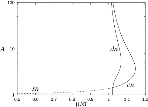
1 10 100

0.5 0.6 0.7 0.8 0.9 1 1.1 1.2

A

µ/σ

sn

cn

dn

Figure 8. The bifurcation diagram for (3.21)–(3.22) with periodic boundary conditions withL= 10π, showing dn, cn (both solid lines) and sn (dashed line) solution branches. The vertical axis shows the maximum value ofA.

A bifurcation diagram showing all three types of solution (cn, dn and sn) is given in figure 8. Note that only the dn solutions bifurcate from the periodic rolls represented byA= 1.

The solutions described above are those containing the minimal number of peaks and troughs within the periodic domain. Other solutions, containingnsets of peaks and troughs can also be constructed by replacing K by nK in the last equation of (3.28), (3.35) or (3.38).

4. Numerical simulations of a model PDE

(a)

-0.4 -0.2 0 0.2 0.4

(b)

-0.4 -0.2 0 0.2 0.4

(c)

-0.4 -0.2 0 0.2 0.4

(d)

-0.4 -0.2 0 0.2 0.4

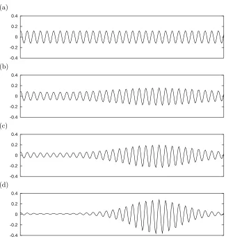
Figure 9. Numerical simulations of (2.7) showing w(x), with r = 0.01 and periodic domain size 62π. (a) Stable rolls,s= 0.9; (b) Modulated rolls,s= 0.93; (c)s= 0.95; (d)s= 1.0.

conditions. From the analysis of _§ 2.2, the system is governed by the amplitude equations (2.5)–(2.6) with

σ=1

4 and µ=

s2

3₋2s2_/9. (4.1)

A pseudospectral method is employed in which the nonlinear terms are computed in physical space using FFTs. Time advancement is carried out by approximating the nonlinear terms as a linear function of time and then obtaining exact solutions using the known growth rate of the linear terms (2.8).

is supercritical. In the limit of large Lthe condition (3.9) for rolls to be unstable is

µ > σ, which is equivalent to s2 _{>27/38. For finite L the condition is (3.6), which} yieldsµ > σ(1 + 2π2_/L2_{), or |s|>0.9215 forL= 3.1π. In our numerical simulations} of (2.7) atr = 0.01, we find good agreement with this asymptotic result, rolls being unstable for_|s_|>0.927.

A sequence of numerical solutions of (2.7) with r = 0.01 for different values of

sis shown in figure 9. In all cases, the solution shown is the final steady state after all transients have decayed; to reach this state the computation must be continued for several thousand time units. In figure 9(a),s= 0.9 and a stable periodic solution is found. For s = 0.93 (figure 9(b)), slightly beyond the bifurcation, a modulated pattern appears. The amplitude of the modulation is small, which is consistent with the result of_§3.2 that the bifurcation is supercritical. Assis increased, the amplitude of the modulation steadily increases (figure 9(c,d)), until there are regions in which the pattern is almost completely suppressed and regions in which the amplitude of the pattern becomes large. The envelope of the pattern takes the form of the dn or sech solutions described in§3.3 (see figure 4); we have not found any of the cn or sn solutions, which suggests that they are unstable.

The increasing amplitude of these solutions means that the numerical simulations are no longer within the asymptotic regime of validity of the equations (2.5)–(2.6); in particular, for this value of r we do not find the saddle–node bifurcation, which, according to (3.26), should occur whens= 0.939 in (2.7).

To find this saddle–node bifurcation it is necessary to carry out further sequences of numerical simulations at smaller values of r. In order to keep the value of L

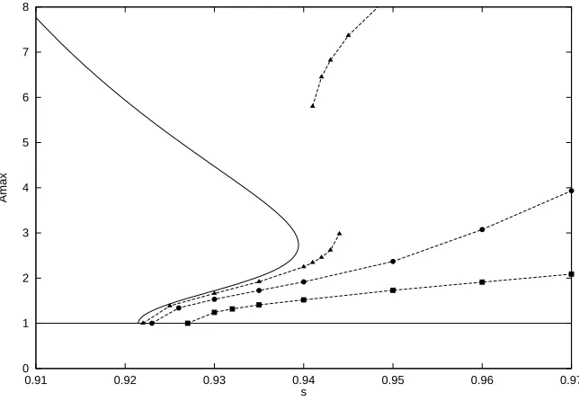
constant, the length of the domain (and the number of grid points) must be increased in proportion to r−1/2_{. The numerically obtained bifurcation diagrams, with r} successively reduced by a factor of 4, are compared with the solution of the amplitude equations in figure 10. The function A is obtained numerically from the part of the spectrum of the numerical solution neark= 1 and scaled appropriately withr1/2_{. For} a domain size 62πwithr= 0.01 there is no saddle–node bifurcation and the numerical and theoretical bifurcation diagrams are not in close agreement. With a domain size 124πandr= 0.0025, agreement is better near the pitchfork bifurcation but there is still no saddle–node bifurcation. Finally, for a domain size 248πwith r= 0.000625 a saddle–node bifurcation appears at s= 0.944, close to the theoretical value of 0.939. Beyond this point the numerical results jump to a solution of much larger amplitude, and there is a region of hysteresis where two stable solutions exist.

0 1 2 3 4 5 6 7 8

0.91 0.92 0.93 0.94 0.95 0.96 0.97

Amax

s

Figure 10. Comparison of the solution to the amplitude equations (2.5)–(2.6) withL= 3.1π(solid line) and numerical solutions for the same value ofLwith three different values of r. Squares: r = 0.01; circles: r = 0.0025; triangles: r= 0.000625.

(a)

-2 -1 0 1

(b)

-2 -1 0 1

results indicates that the multi-pulse solutions are not quite stationary; the pulses are gradually moving.

5. Beyond the leading-order amplitude equations

In the previous section we have seen that agreement between the amplitude equations (2.5)–(2.6) and the behaviour of the full PDE (2.7) only occurs for extremely small values ofr. This agreement can be improved by introducing higher-order terms into (2.5)–(2.6). Rather than include all possible terms that might arise at the next order in (2.5)–(2.6), we focus on one term.

To motivate our choice of higher-order term, we note that when we compute the

x-average ofw3_{, the leading-order contribution is}4₍2 3s|A|

4_{+ 6}

|A_|2_{B). For moderate} values ofs, the term 64

|A_|2_{B dominates. After rescaling the equations forAandB} so thatAsatisfies (2.5), we find thatB satisfies

BT =σBXX +µ(|A|2)XX+δ(B|A|2)XX, (5.1)

whereσandµare given by (4.1) and

δ= 3 2

2 3₋2 9s2

>0. (5.2)

For future convenience we introduce the quantityM, defined by

h(M ₋µ0_|A_|2)/(1 +δ_|A_|2/σ)_i= 0. (5.3) When µ0>0, the term inδ plays a stabilising role.

For steady solutions, the governing equation forAbecomes

0 =A+AXX −A|A|2−A

M−µ0|A|2 1 +δ|A|2_/σ

. (5.4)

The bifurcation diagram for this equation, subject to the constraint (5.3), is indicated in figure 12. The bifurcation diagram is changed significantly even by very small values ofδ. For example, whereas there is a single saddle–node bifurcation for δ = 0, when

δ > 0 there is a pair of saddle–node bifurcations. This pair exists only forδ/σ less than approximately 0.0009, and for larger values of δ/σthe curve is monotonic.

We now wish to determine the effect of smallδ upon the envelope of the pattern, since our numerical simulations suggest that the envelope will broaden from a sech profile as the envelope becomes more developed. For smallδ, (5.4) is approximately

0 = (1₋M)A+AXX−(1−µ0−δM/σ)A|A|2−µ0δA|A|4/σ. (5.5)

and so to determine the effect ofδ upon the envelope, it is instructive to examine the model equation

f00=f−f3+δf5. (5.6)

This model contains the essential features of the problem (5.3) and (5.5) forA, and has the exact solution

f =b1/2 1

4(b−2) + cosh

2_x−1/2_{, (5.7)}

1 2 3 4 5 6 7 8 9 10

1.06 1.08 1.1 1.12 1.14 1.16 1.18 1.2 1.22 1.24

A

µ/σ

Figure 12. Bifurcation diagram for (5.4) subject to (5.3) forδ/σ= 10−4(solid line), 10−3 _{(dashed line) and 10}−2 _{(dotted line) plotted using AUTO97. The}

domain length is L = 5π. Note that very small values of δ can change the qualitative nature of the bifurcation diagram, for example eliminating the saddle– node bifurcation atδ= 0.

0 1 2

-8 -6 -4 -2 0 2 4 6 8

f

x

Figure 13.Envelopes (5.7) from the model equation (5.6) withδ= 0 (solid line) andδ= 0.185 (dashed line). The larger value ofδproduces a broad profile with a nearly uniform region in whichf is non-zero. The broader profile is reminiscent of the envelope in figure 11.

6. Examples

Since conservation laws arise very commonly in nature, it turns out that a wide variety of pattern formation problems are governed by the system (2.5)–(2.6) rather than the Ginzburg–Landau equation alone.

and Matthews (2000), (2.5)–(2.6) appear as a special case, and it can be shown that rotating convection is unstable for moderate values of the Prandtl number.

In Marangoni convection (driven by surface tension), the fluid has a free surface and the equation for the layer depth is constrained by conservation of mass. Equations similar to (2.5)–(2.6), but with one extra term, were derived by Golovin, Nepomnashchy and Pismen (1994); in this case, however, the parameterµis negative and so no instability arises.

In_§§6.1 and 6.2 below, we derive an equation similar to (2.7) for two problems in convection; in_§ 6.3, we directly derive amplitude equations equivalent to (2.5)–(2.6) for magnetoconvection between ‘ideal’ horizontal boundaries.

6.1. Application to convection with a nonlinear equation of state

A physical problem that gives rise to amplitude equations of the form considered here is convection between boundaries at which the heat flux is fixed (Roberts 1985, Matthews 1988a, 1988b). The fluid has a nonlinear equation of state,

ρ_∗=ρ01−α(T∗−T0)−β(T∗−T0)2, (6.1)

relating the fluid densityρ∗ to the temperature T∗. The coefficients α, β andT0 are constants. This equation of state is appropriate for water around 4◦C, for example. The crucial feature of this problem is that the total heat in the layer is conserved; the fixed-flux boundary conditions allow a large-scale, slowly-evolving depth-averaged temperature mode, Θ.

We suppose that the temperature profile is nonlinear, of the form (Matthews 1988a, 1988b):

T∗=T0+Az_∗3− Bz∗, (6.2)

wherez∗is the vertical coordinate. The problem is expressed in dimensionless variables by adopting the scalesd= (_B/_A)1/2_,

Bdandd2_{/κ for length, temperature and time.} We then find the equations governing two-dimensional motions to be

P−1 ∇2ψt+J(ψ,∇2ψ) =Rθx+∇4ψ+R∆(z3−z+θ)θx, (6.3)

θt+J(ψ, θz) + (3z2−1)ψx=∇2θ, (6.4)

where the x- and z-components of velocity may be expressed in terms of the streamfunction ψ as (u, w) = (₋ψz, ψx), and the Jacobian is defined by J(f, g) =

fxgz−fzgx. The perturbation to the temperature profile (6.2) is denoted byθ. The

Rayleigh number is

R= gαBd 4

νκ ,

whereνandκare, respectively, the coefficient of kinematic viscosity and the coefficient of thermal diffusivity, g is the gravitational acceleration; the Prandtl number is

P =ν/κ, and ∆ = 2_Bdβ/α. In deriving the PDE for Θ, we assume that the equation of state is only mildly nonlinear, so that_|∆_| 1.

We break the up–down symmetry of the problem by imposing rigid boundary conditions atz=₋H but stress-free conditions atz=H. Thus

ψ=ψz= 0 at z=−H (6.5)

and

R

1

k

1

R

k

0

H>H

0

R

H<H

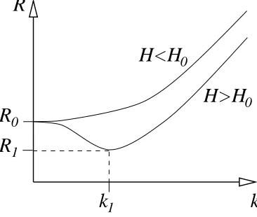
Figure 14. Marginal stability curves for convection with a nonlinear equation of state and nonlinear basic-state temperature profile. When the depthH of the fluid layer is less than some thresholdH0, the critical wavenumber is zero and

the critical Rayleigh number isR0, given by (6.7); whenH > H0, the critical

wavenumberk1is positive, and the critical Rayleigh numberR1is less thanR0.

The important mathematical consequence of these boundary conditions is that the equation for Θ then contains a quadratic nonlinear term of the form (Θ2

X)XX, where

X is a scaled x-coordinate. This term tends to lead to a supercritical bifurcation to rolls, unlike the quadratic term (Θ2₎

XX, which arises from the nonlinear equation of

state, and which tends to lead to a subcritical bifurcation.

We suppose that the heat flux through the planes z=_±H is fixed, so that the perturbation heat flux ∂θ/∂z = 0 at each boundary. The key consequence of this choice of boundary condition is that, for sufficiently small half-depthH, the critical mode of the linear stability problem has zero wavenumber (see figure 14).

We begin by considering the simpler case of a linear equation of state, with ∆ = 0. First we examine equations (6.3)–(6.4), linearised about the trivial state ψ=θ= 0. We find, making asymptotic expansions of the forms given by Roberts (1985) and Matthews (1988a), that modes with wavenumberkhave linear growth rateλ, where

λ∼(R−R0)R0−1k2−a4k4, R0= 420H−4(11H2−21)−1,(6.7) for small|R−R0|andk. The coefficienta4 is

a4=

8H2_(6831H4

−25738H2_{+ 23751)} 1287(11H2₋₂₁₎2 .

As a consistency check on these results, we note that as H _→ 0, R0 ∼ 20/H4 and

a4∼232H2/693. This limit corresponds to the problem with a linear equation of state and linear basic-state temperature profile, such as considered by Chapman and Proctor (1980). After appropriately rescaling of the depth of our fluid layer, we find that their results agree with ours in the limit asH_→0. When a4>0, the largest wavenumbers in (6.7) are damped, and k= 0 corresponds to a minimum of the marginal stability curve. This condition is satisfied for 0< H < H0, where H0≈1.2709 is the smaller positive root ofa4= 0 (see figure 14).

The amplitude equation of interest applies whenHis close toH0. We thus follow Roberts (1985) and Matthews (1988a) and let

expanding the streamfunction and temperature perturbation as

θ =2θ2(X, T) +2θ4(X, z, T) +· · · (6.9)

ψ=3_{ψ3(X, z, T) +}2_{ψ5(X, z, T) +}

· · ·, (6.10)

where X = xand T =6_{t. These scalings have been adopted to ensure a balance} of terms in the equation derived below. Of course, it is reasonable to question the physical relevance of such a large power of in the scaling of time, and we offer two partial justifications. The first is that, in fact, solutions to model PDEs of the form to be derived below are known to provide a good approximation to the full convection problem even when is not particularly small (and hence 6 _{represents a physically} achievable scaling). The second justification is that in deriving amplitude equations of the form (2.5)–(2.6) it is notnecessaryto pass through an intermediate stage involving the time scale6_{t, this is just a convenient way to construct in an asymptotic fashion} a long-wavelength model PDE.

At O(2_{) in (6.3)–(6.4), we find that ∂}2_θ

2/∂z2 = 0, subject to the boundary conditions∂θ2/∂z = 0 at z = ±H. The solution for θ2 is therefore independent of depth, as indicated in (6.9). After some algebra, we find from a solvability condition atO(8_{) that the amplitude equation for Θ =θ2(X, T) is}

ΘT =

−R_R4

0

+a2D2

Θ + (a04H2+a004D)ΘXX +a6ΘXXXX +aqΘ2X−12DΘ 2

XX

(6.11)

where the numerical values of the coefficients in (6.11) are given approximately by

a2 = 7.588×10−5, (6.12)

a04 = 8.966, (6.13)

a004 = 0.1208, (6.14)

a6 = 0.3067, (6.15)

aq = 5.571−1.086/P, (6.16)

R0= 49.80. (6.17)

To ensure that all terms in the equation for ΘT arise at the same asymptotic order,

R2=a7D, where a7≈0.4338.

After rescaling, we can write (6.11) as

∂w ∂t =−

∂2

∂x2 "

rw−

1 + ∂ 2

∂x2 2

w−sw2− _∂w

∂x

2#

, (6.18)

which is very similar in form to (2.7) considered in _§ 2.2. Following the asymptotic procedure outlined in_§ 2.2, we find that withw(x, t) as in (2.10), the amplitudes of the pattern and large-scale modes satisfy

AT =r2A+ 4AXX−2(1−s)(s+ 2)A|A|2/9−2sAB, (6.19)

BT =BXX + 2(s+ 1)(|A|2)XX. (6.20)

If ₋2 < s < 1, the coefficient of the term A_|A_|2 _{in (6.19) is negative, and the} bifurcation to pattern (in the absence of B) is supercritical. Equations (6.19) and (6.20) are then equivalent to (2.5)–(2.6), after an appropriate rescaling.

From this analysis we find that the bifurcation to rolls is supercritical if ₋2 < s <1, and that all rolls are unstable if

−2< s <−1₂−3 √

57

38 ≈ −1.096 or 0.096≈ − 1 2+

3√57

where

s= a

1/2

6 R

1/2

0 ∆

2aq(R0+a7∆ +a2R0∆2−R)1/2

. (6.22)

6.2. Application to thermosolutal convection

As a second physical example, we examine thermosolutal convection between boundaries at which the heat flux is fixed. We suppose that the fluid is slightly non-Boussinesq, so that the thermal diffusivity is a weak function of the local temperature:

κ∗=κ0(1 + ˆκ(T∗−T0)/T0). (6.23)

The layer is heated from below and in the basic state the saltier water lies over the fresher water, so both mechanisms are destabilising. Both the thermal and the solutal gradients are vertical and uniform in the absence of convection. The thermal gradient is characterised by a (thermal) Rayleigh number R >0 and the salinity gradient by a solutal Rayleigh numberS < 0. When 0> S > Sc, the bifurcation to convection

takes place at zero wavenumber; when Sc > S, the critical wavenumber is finite. We

analyse the case

S=Sc+2S2.

The natural scale for lengths is now the depth of the layer, and that for temperature perturbations is the temperature difference across the layer in the basic state (similarly for the salt concentration). With these scales, the dimensionless governing equations may be written in the form

P−1 ∇2_ψ

t+J(ψ,∇2ψ) =Rθx−SΣx+∇4ψ (6.24)

θt+J(ψ, θ)−ψx =∇2θ+ ˆκ∇·[(−z+θ)∇θ] (6.25)

Σt+J(ψ,Σ)−ψx =τ∇2Σ, (6.26)

where Σ is the perturbation salinity field,τ =κs/κandκsis the salt diffusivity. The

thermal Rayleigh number is now

R= gα(dT∗/dz∗)d 4

νκ0

, (6.27)

where α is the coefficient of cubical expansion and dT_∗/dz_∗ is the (dimensional) temperature gradient in the absence of convection; the solutal Rayleigh number S

is defined similarly.

As in the previous example, we use free–rigid horizontal boundary conditions, with (6.5) and (6.6) applied forH= 1/2, since the fluid layer now has unit dimensionless depth. With these boundary conditions,Sc=−8352τ /41≈ −203.707τ.

The amplitude equation of interest applies when

R=R0+4R4, S=Sc+2S2, κˆ=2κ2;

we expand the independent variables as

θ =2_{θ2(X, T) +}2_{θ4(X, z, T) +}

· · · (6.28)

Σ =4Σ4(X, z, T) +2Σ6(X, z, T) +· · · (6.29)

whereX=xandT =6_{t. AtO(}8_{) in an asymptotic expansion of (6.24)–(6.26), we} find that the amplitude equation for Θ =θ2(X, T) is

ΘT =

−R_R4

0

Θ +c4S2ΘXX +c6ΘXXXX +cqΘ2X+12κ2Θ 2

XX

.(6.31)

where

R0= 320, (6.32)

c4 = − 41

99792τ ≈ −0.0004109/τ, (6.33)

c6 =

14506722953

1105865601750≈0.01312, (6.34)

cq = −

5 + 7P

84P ≈ −0.08333−0.05952/P. (6.35)

Note that this has exactly the same form as (6.18). From _§ 6.1, the condition for a supercritical bifurcation is₋2< s <1, and that for all rolls to be unstable is (6.21), where

s= κcˆ 1/2

6 R

1/2 0 2cq(R0−R)1/2

. (6.36)

6.3. Application to magnetoconvection

Convection in a vertical magnetic field has been a subject of a great deal of research (see, for example, Proctor and Weiss 1982; Matthews 1999). The problem is motivated by the convection zone of the Sun, where the magnetic field is moved around by the fluid and regions of strong magnetic field inhibit the fluid motion. In the nonlinear regime magnetoconvection exhibits a very wide range of complicated phenomena.

In magnetoconvection, the conservation law that leads to the large-scale mode is that the total flux of magnetic field through the layer is conserved. The governing equations for two-dimensional magnetoconvection are (Proctor and Weiss 1982), in the notation of the preceding section,

P−1 ∇2_ψ

t+J(ψ,∇2ψ) =R θx+∇4ψ+ζQ J(φ,∇2φ) +∇2φz, (6.37)

θt+J(ψ, θ) =ψx+∇2θ, (6.38)

φt+J(ψ, φ) =ψz+ζ∇2φ. (6.39)

The magnetic field is defined through a perturbation flux functionφ by (Bx, Bz) =

(₋φz,1 +φx). The parameter Q is the Chandrasekhar number, a dimensionless

measure of the magnetic field strength, while ζ is the ratio of magnetic diffusivity to thermal diffusivity.

The most commonly used boundary conditions are that the upper and lower boundaries are stress free, fixed temperature and with no horizontal magnetic field, so

ψ=ψzz =θ=φz= 0 at z= 0,1. (6.40)

These boundary conditions are convenient in the sense that the linear eigenfunctions are trigonometric.

The large-scale mode in the problem arises through a rearrangement of the vertical magnetic field. There is a linear eigenfunction in whichφ=φ(x, t) which obeys the diffusion equationφt=ζφxx, so the growth rateλ of a mode with wavenumberkis

perturbation, since if φ = φ(x, t) there is no forcing term in (6.37). Although this mode is usually ignored in the analysis of magnetoconvection, it plays a crucial role when the horizontal size of the domain is large. Note that although there are nearly marginal modes at small k and at order-one values of k, the graph of growth rate versus wavenumber is not as shown in figure 1, because the large-scale mode and the order-one mode correspond to two distinct branches of eigenfunctions.

The weakly nonlinear analysis proceeds by including the large-scale mode. The general analysis of_§2 suggests that the mean mode should be included at order 2_. In fact the mean vertical magnetic field is of order 2 _{and so the corresponding flux} functionφis of order . The appropriate asymptotic expansions near the stationary bifurcation to convection are therefore

ψ=A(X, T) exp ikxsinπz+c.c.+O(2), (6.41)

θ =A(X, T)θ1i exp ikxsinπz+c.c.+O(2_{), (6.42)}

φ=A(X, T)φ1exp ikxcosπz+c.c.+ φ1Φ(X, T) +O(2), (6.43) whereθ1 and φ1 are constants, readily determined from the linear stability problem,

X = x, T = 2t and R = Rc +2R2. At order we obtain θ1 = k/(π2 +k2),

φ1=π/ζ(π2+k2) and the well known result (Chandrasekhar 1961)

Rc= (π

2_+k2₎3_+Qπ2_(π2_+k2₎

k2 . (6.44)

From (6.44) it follows that as Ris increased, convection first occurs with a critical wavenumberkc which is related toQby

Qπ4= (2k2_c−π2)(π2+k2_c)2. (6.45) Henceforth it is assumed thatk=kc; note that the envelope functionA(X, T) permits

convection with a wavenumberk=kc+O().

At order 2_{, a term in θ proportional to sin 2πz and a φ term proportional to} exp 2ikxare obtained. At third order, evolution equations forA and Φ are found by applying solvability conditions. Full details of the calculation will be given elsewhere. The resulting amplitude equations are

AT =a1A+a2AXX−a3A|A|2−a4AΦX, (6.46)

ΦT =ζΦXX +π |A|2

X, (6.47)

wherea1. . . a4are known constants, given by cumbersome functions of the parameters;

a2 and a4 are always positive. After setting ΦX = B, (6.46)–(6.47) are equivalent

to (2.5)–(2.6). The equations (6.46)–(6.47) have not been derived previously, but the underlying processes of the coupling between the convection rollsAand the large-scale mode Φ are well understood (see, for example, Proctor and Weiss 1982). Sincea4>0, the coupling term in (6.46) simply reflects the fact that the magnetic field suppresses convection. The coupling term in (6.47) describes the process of flux expulsion: the magnetic field strength decreases in regions where the convection is strong.

The bifurcation at the onset of convection is supercritical (i.e.a3>0) provided that

k4ζ2(π2+k2)> π2(2k2₋π2)(π2₋k2), (6.48) whereQhas been eliminated in favour ofk using (6.45). The result (3.9) can now be applied to determine whether a regular pattern of rolls is unstable. It is found that all rolls are unstable if

k4_ζ2_(π2_+k2_{)< π}2_(2k2

0.1 1 10 100 1000 10000 100000 1e+06

0 0.5 1 1.5 2

Q

ζ

Subcritical

Unstable rolls Stable rolls

Figure 15. Region of stability of convection rolls in magnetoconvection. To the right of the solid line, rolls are stable. To the left of the dashed line the bifurcation is subcritical. Between the two lines, all rolls are unstable.

where Qhas again been eliminated using (6.45). Note that neither of the conditions (6.48)–(6.49) involves the Prandtl number P. Using k as a parameter, the region of stability of rolls can be plotted in the Q, ζ plane (figure 15). In the small region where the rolls are subcritical the weakly nonlinear analysis gives no useful information about the pattern. However, there is a large region of parameter space in which the bifurcation is supercritical but all rolls are unstable. In this region we expect to find that the stable pattern at onset consists of rolls that are modulated on a large length-scale. Solutions of this type, but fully nonlinear, have recently been obtained through numerical simulations of magnetoconvection (Blanchflower 1999).

Note that our analysis is confined to the onset of convection at a stationary bifurcation. For certain parameter values (in general, whenQis large andζ is small) the onset of magnetoconvection is oscillatory; since this depends on the value of P, this condition is not shown in figure 15.

7. Discussion

We have derived amplitude equations (2.5)–(2.6) for the primary bifurcation to a stationary pattern in a one-dimensional system with a conservation law for a quantity that does not change sign under reflection. In this case the conservation law leads to a neutral large-scale mode which must be taken into account for a correct description of the behaviour near onset. The usual Ginzburg–Landau equation (Melbourne 1999) is coupled to an equation describing the large-scale evolution of the conserved quantity. We have shown how these equations may be obtained from symmetry considerations alone, and have also derived them directly from the governing equation(s) of the system.

is an amplitude-driven instability (whereas the Eckhaus instability is phase-driven) and it is in general supercritical. Most importantly, for certain parameter values

all patterns are unstable. Our instability is also different from that which occurs in the case where the conserved quantity is velocity-like, and the reflection symmetry acts as₋1 (such as in systems with Galilean invariance), where periodic patterns are always unstable and chaotic dynamics is observed at onset (Tribelsky and Velarde 1996, Tribelsky and Tsuboi 1996, Matthews and Cox 2000).

Beyond the instability, there are stable solutions in the form of a strongly amplitude-modulated periodic pattern, the envelope of which we have calculated in terms of Jacobi elliptic functions. The envelope may commonly be approximated by a sech profile. Numerical simulations reveal that these strongly modulated patterns may be stable in the full governing PDE, not just within the framework of the amplitude equations. Numerical simulations of the governing PDE also demonstrate that the amplitude equations represent a good approximation provided the amplitude is sufficiently small, but that higher-order terms play an important role as the amplitude increases; these higher-order terms can lead to significant modifications in the bifurcation diagram, and a broadening of the envelope of the pattern.

Our work demonstrates that localised solutions are possible when a Ginzburg– Landau equation is coupled to an equation for a mean field, even when the coefficients of the equations are real and when the bifurcation is supercritical. Previous work has required complex coefficients (Riecke 1992a, 1992b, Sakaguchi 1993), a subcritical bifurcation (Herrero and Riecke 1995, Sakaguchi and Brand 1996) or both. Our amplitude equations apply when the bifurcation from the basic state is stationary; the case of oscillatory bifurcation to travelling-wave solutions has been analysed in a series of papers by Riecke and co-workers (Riecke 1992a, 1992b, 1996, Herrero and Riecke 1995) and by others (Sakaguchi 1993, Barthelet and Charru 1998), who find a variety of localised and front-type solutions. They find that the coupling to a mean field (our B) can have a significant effect on solutions and their stability, and can stabilise localised travelling-wave trains, and holes.

We have applied our amplitude equations to three convection problems, leading to novel instabilities in these systems. Further details of these applications will be given elsewhere. In the first two, the heat flux is fixed on the boundaries, and the total heat in the layer is conserved, which leads to a large-scale mode in the form of a depth-averaged temperature perturbation. However, in order for our amplitude equations (2.5)–(2.6) to apply, this large-scale mode must influence the convection rolls; this is achieved by using either a nonlinear equation of state or a temperature-dependent diffusivity. In the third example, magnetoconvection, the conserved quantity is the vertical magnetic field; in this case the large-scale mode and the pattern mode correspond to two distinct branches of eigenfunctions of the linear problem. Our modulated solutions may be related to the isolated ‘convectons’ found recently in magnetoconvection (Blanchflower 1999). Another application of our work is in rotating convection, where the conserved quantity is momentum (Cox and Matthews 2000).

spatial period of the perturbation and the basic pattern are irrationally related, A

may be complex. Our results suggest that if a pattern of wavelength L undergoes a supercritical subharmonic bifurcation then there may be stable states where the original pattern is largely undisturbed in some regions but where the perturbation is strong in others. Furthermore, provided the secondary bifurcation is supercritical, it should be possible to find stable states consisting of two domain types: in one domain the pattern is essentially the basic cellular state, in the other the pattern is strongly perturbed.

It would be of interest to investigate how this theory may be extended to problems in two or three space dimensions; in particular we would like to know whether solutions may be obtained that are localised in space. Such localised solutions have been found experimentally by VanHooket al.(1995, 1997). Localised solutions after an oscillatory bifurcation have recently been examined in two dimensions by Riecke and Granzow (1998), who found that such solutions may be obtained in a pair of Ginzburg–Landau equations coupled to a mean-field equation. Of particular interest is their result that stable localised states can be found, as here, when the primary bifurcation is supercritical and the coefficients of the amplitude equations are real.

Acknowledgments

We have benefited from useful discussions with Richard Tew on the subject of Jacobi elliptic functions.

References

Abramowitz M and Stegun I A 1965Handbook of Mathematical Functions(New York: Dover). Barthelet P and Charru F 1998 Benjamin–Feir and Eckhaus instabilities with Galilean invariance:

the case of interfacial waves in viscous shear flowsEur. J. Mech. B171–18. Blanchflower S 1999 Magnetohydrodynamic convectonsPhys. Lett. A26174–81. Chandrasekhar S 1961Hydrodynamic and hydromagnetic stability(New York: Dover).

Chapman C J and Proctor M R E 1980 Nonlinear Rayleigh–B´enard convection between poorly conducting boundariesJ. Fluid Mech.101759–782.

Charru F and Barthelet P 1999 Secondary instabilities of interfacial waves due to coupling with a long wave mode in a two-layer Couette flowPhysicaD 125311–324.

Cox S M 1998 Long-wavelength rotating convection between poorly conducting boundariesSIAM J. Appl. Math.581338–1364.

Cox S M and Matthews P C 2000 Instability of rotating convectionJ. Fluid Mech.403153–172. Cross M C and Hohenberg P C 1993 Pattern formation outside of equilibriumRev. Mod. Phys.65

851–1112.

Coullet P and Fauve S 1985 Propagative phase dynamics for systems with Galilean invariancePhys. Rev. Lett.552857–2859

Coullet P and Iooss G 1990 Instabilities of one-dimensional cellular patternsPhys. Rev. Lett. 64

866–869.

Eckhaus W 1965Studies in Non-linear Stability Theory(New York: Springer).

Fauve S 1987 Large scale instabilities of cellular flows. In Instabilities and nonequilibrium structures, ed. E. Tirapegui and D. Villarroel, 63–88.

Golovin A A, Nepomnashchy A A and Pismen L M 1994 Interaction between short-scale Marangoni convection and long-scale deformational instabilityPhysics of Fluids634–48.

Herrero H and Riecke H 1995 Bound pairs of fronts in a real Ginzburg–Landau equation coupled to a mean fieldPhysicaD 8579–92.

Hidaka Y, Huh J-H, Hayashi K-i, Kai S and Tribelsky M I 1997 Soft-mode turbulence in electrohydrodynamic convection of a homeotropically aligned nematic layerPhys. Rev E 56

R6256–R6259.

Matthews P C 1988b A model for the onset of penetrative convectionJ. Fluid Mech.188571–583. Matthews P C 1998 Hexagonal patterns in finite domainsPhysicaD 11681–94.

Matthews P C 1999 Asymptotic solutions for nonlinear magnetoconvectionJ. Fluid Mech.387397– 409.

Matthews P C and Cox S M 1999 Pattern formation with Galilean invariancesubmitted.

Melbourne I 1999 Steady-state bifurcation with Euclidean symmetryTrans. Amer. Math. Soc.351

1575–1603.

Proctor M R E and Weiss N O 1982 MagnetoconvectionRep. Prog. Phys.451317–1379.

Riecke H 1992a Self-trapping of traveling-wave pulses in binary mixture convectionPhys. Rev. Lett. 68301–304.

Riecke H 1992b Ginzburg–Landau equation coupled to a concentration field in binary-mixture convectionPhysicaD 61253–259.

Riecke H 1996 Solitary waves under the influence of a long-wave modePhysicaD 9269–94. Riecke H and Granzow G D 1998 Localization of waves without bistability: worms in nematics

electroconvectionPhys. Rev. Lett. 81 333–336.

Roberts A J 1985 An analysis of near-marginal, mildly penetrative convection with heat flux prescribed on the boundariesJ. Fluid Mech.15871–93.

Sakaguchi H and Brand H R 1996 Stable localized solutions of arbitrary length for the quintic Swift– Hohenberg equationPhysicaD 97274–285.

Swift J B and Hohenberg P C 1977 Hydrodynamic fluctuations at the convective instabilityPhys. Rev. A15 319–328.

Tribelsky M I and Velarde M G 1996 Short-wavelength instability in systems with slow long-wavelength dynamics.Phys. Rev. E544973–4981.

Tribelsky M I and Tsuboi K 1996 New scenario for transition to turbulence? Phys. Rev. Lett. 76

1631–1634.

Tuckerman L S and Barkley D 1990 Bifurcation analysis of the Eckhaus instabilityPhysica D 46

57–86.

VanHook S J, Schatz M F, McCormick W D, Swift J B and Swinney H L 1995 Long-wavelength instability in surface-tension-driven B´enard convectionPhys. Rev. Lett.754397–4400. VanHook S J, Schatz M F, Swift J B, McCormick W D, and Swinney H L 1997 Long-wavelength