Force free collisionless current sheet models with non uniform temperature and density profiles

Force-free collisionless current sheet models with non-uniform temperature

and density profiles

F.Wilson,1,a)T.Neukirch,1and O.Allanson1,2

1

School of Mathematics and Statistics, University of St. Andrews, St. Andrews KY16 9SS, United Kingdom

2

Space and Atmospheric Electricity Group, Department of Meteorology, University of Reading, Reading RG6 6BB, United Kingdom

(Received 26 July 2017; accepted 2 August 2017; published online 17 August 2017)

We present a class of one-dimensional, strictly neutral, Vlasov-Maxwell equilibrium distribution functions for force-free current sheets, with magnetic fields defined in terms of Jacobian elliptic functions, extending the results of Abraham-Shrauner [Phys. Plasmas20, 102117 (2013)] to allow for non-uniform density and temperature profiles. To achieve this, we use an approach previously applied to the force-free Harris sheet by Kolotkovet al.[Phys. Plasmas22, 112902 (2015)]. In one limit of the parameters, we recover the model of Kolotkov et al. [Phys. Plasmas 22, 112902 (2015)], while another limit gives a linear force-free field. We discuss conditions on the parameters such that the distribution functions are always positive and give expressions for the pressure, den-sity, temperature, and bulk-flow velocities of the equilibrium, discussing the differences from pre-vious models. We also present some illustrative plots of the distribution function in velocity space. VC _{2017 Author(s). All article content, except where otherwise noted, is licensed under a Creative} Commons Attribution (CC BY) license (http://creativecommons.org/licenses/by/4.0/).

[http://dx.doi.org/10.1063/1.4997703]

I. INTRODUCTION

Force-free current sheets, with magnetic fields satisfying

r B¼0; (1) r B¼l0j; (2)

jB¼0; (3)

are appropriate for plasma modelling in, e.g., the solar atmo-sphere and planetary magnetoatmo-spheres (e.g., Refs. 3–15). Equations(1)–(3)imply that the current density is parallel to the magnetic field:j¼aðrÞB. The case wherea ¼ 0 defines a potential field, and when a is constant, we have a linear force-free field. Whenavaries with the positionr, the field is referred to as nonlinear force-free.

Such current sheets as described earlier can play a cru-cial role in, e.g., magnetic reconnection processes, for which it is often necessary to consider kinetic length scales (e.g., Ref. 16), since many astrophysical plasmas are approxi-mately collisionless. To initialise the studies of collisionless reconnection, a Vlasov-Maxwell (VM) equilibrium can be used; since current sheets are strongly localised, they are often well described by one-dimensional (1D) VM equilib-rium models. The work by Wilsonet al.17was the first exam-ple of a study of collisionless reconnection for which an exact nonlinear force-free equilibrium was used in the initial setup, using a distribution function (DF) found by Harrison and Neukirch18for the “force-free Harris” current sheet

B¼B0ðtanhðz=LÞ;sechðz=LÞ;0Þ: (4)

Other studies of collisionless reconnection in force-free cur-rent sheets have involved the use of approximate force-free equilibria (e.g., Refs. 19–26) or linear force-free equilibria (e.g., Refs.27–29).

To find VM equilibrium DFs consistent with force-free current sheets involves solving the VM equations in the opposite order from what is usually done; a magnetic field satisfying Equations (1)–(3) is specified, and the DFs are then given by the solution of an inverse problem (e.g., Refs. 30–33). As such, finding exact force-free VM equilibria is generally a non-trivial task, and this is reflected in the rela-tively small number of known solutions. Linear force-free VM equilibria have been discussed in, e.g., Refs.18,27,31, and34–37. The first solution for a nonlinear force-free field was found by Harrison and Neukirch38(see also Ref.39) for the force-free Harris sheet, and these solutions were later extended by Kolotkovet al.2to allow for non-uniform den-sity and temperature profiles (with respect to the spatial coor-dinate). A number of other equilibrium DFs have also been found for this field. Wilson and Neukirch40found DFs with an arbitrary dependence on the particle energy; Stark and Neukirch41 discussed DFs in the relativistic limit; Allanson

et al.33,42found DFs in terms of infinite sums over Hermite polynomials, with an arbitrarily low plasma beta (in the pre-vious work on the force-free Harris sheet, the plasma beta was constrained to be greater than unity); Dorville et al.43

discussed “semi-analytic” DFs for a magnetic field, which includes the force-free Harris sheet as a special case.

Abraham-Shrauner1discussed VM equilibria for a non-linear force-free magnetic field given in terms of Jacobian elliptic functions. This work can be thought of as a generali-sation of some of the previous work, to account for both lin-ear and nonlinlin-ear force-free equilibria in one model, since,

a)

Electronic mail: [email protected]

1070-664X/2017/24(9)/092105/11 24, 092105-1 VCAuthor(s) 2017.

in one limit of the elliptic modulus, the magnetic field becomes the force-free Harris sheet field, and in another limit, it becomes a linear force-free field. The DFs discussed give rise to spatially uniform temperature and density pro-files, in a similar way to some of the models mentioned above. In this paper, we will extend this class of DFs to include those consistent with non-uniform temperature and density profiles, using a similar approach used by Kolotkov

et al.2 for the force-free Harris sheet. As for Abraham-Shrauner’s DFs, the new DFs we will discuss include both the linear force-free limit and the force-free Harris sheet limit.2

The paper is laid out as follows; in Sec. II, we outline the background theory of 1D VM equilibria; in Sec.III, we present an overview of the work by Abraham-Shrauner;1we discuss the extension of this work to include non-uniform temperature and density profiles in Sec.IV, and the velocity space structure of the new DFs is discussed in Sec. V; we end with a summary in Sec.VI.

II. 1D VLASOV-MAXWELL EQUILIBRIA

In line with some of the previous work on 1D VM equi-libria (e.g., Refs.18,38, and39), we assume that all quanti-ties depend only on thez-coordinate and that the magnetic field, B¼ ðBx;By;0Þ, can be written as the curl of a vector potential, A¼ ðAx;Ay;0Þ. We will not repeat all of the details here, but the result of the above assumptions is that the problem reduces to solving Ampe`re’s law in the form

d2Ax dz2 ¼ l0

@Pzz

@Ax

; (5)

d2Ay dz2 ¼ l0

@Pzz

@Ay

; (6)

to findPzz, which is thezz-component of the pressure tensor,

defined by

PzzðAx;AyÞ ¼ X

s

ms ð

v2

zfsðHs;pxs;pysÞd3v; (7)

where we assume that the DFs can be chosen in such a way that they are compatible with strict neutrality (the scalar potential/¼0).31Note that we only considerPzzsince this

is the component of the pressure tensor which is important for the force-balance of the 1D equilibrium. The DFs, denoted by fs, are assumed to be functions of the particle

energy, Hs¼msðv2xþv

2

yþv

2

zÞ=2, and the x- and y -compo-nents of the canonical momentum, p¼msvþqsA, since these are known constants of motion for a time-independent system with spatial invariance in the x- and y-directions. Once Ampe`re’s law has been solved forPzz, the DF can be

found by solving Eq. (7). This is an example of an inverse problem.

III. ABRAHAM-SHRAUNER’S MODEL

In this section, we discuss some properties of the model developed by Abraham-Shrauner,1in order to give context to

the discussion we will present in Sec. IV. In Abraham-Shrauner’s work, a nonlinear force-free current sheet profile is considered, described by the magnetic field

B¼B0ðsnðz=LÞ;cnðz=LÞ;0Þ; (8)

whereB0is a constant,L is the current sheet half-thickness, and sn and cn are Jacobian elliptic functions44 with the modulus ksuppressed (where 0k1). In the limit k! 0;snðz=LÞ ! sinðz=LÞand cnðz=LÞ ! cosðz=LÞ, and so the magnetic field (8) becomes the linear force-free field

B¼B0ðsinðz=LÞ;cosðz=LÞ;0Þ. In the limit k!1;snðz=LÞ

!tanhðz=LÞ and cnðz=LÞ !sechðz=LÞ, giving the force-free Harris sheet magnetic field [Eq.(4)]. The vector poten-tial,A, used by Abraham-Shrauner1is given by

Ax¼

B0L

k arcsinðksnðz=LÞÞ þ kp

2

; (9)

Ay¼

B0L k ln

kcnðz=LÞ þdnðz=LÞ 1þk

; (10)

where dn is also an elliptic function. This can be seen by using standard integrals45 and by choosing the integration constants such that, when k!1;Ax!2B0Larctanðez=LÞ; Ay! lnðcoshðz=LÞÞ—the vector potential components used in some of the previous work on the force-free Harris sheet (note also that an alternative gauge forAis discussed for the force-free Harris sheet by Allansonet al.33).

The current density is given by

j¼ B0

l0L

snðz=LÞdnðz=LÞ;cnðz=LÞdnðz=LÞ;0

ð Þ ¼dnðz=LÞB

l0L

;

(11)

and so the force-free parameterais given by

að Þ ¼z dnðz=LÞ

l0L

: (12)

Note that, in the limitk!0;dnðz=LÞ !1, and soais con-stant (the linear force-free case), but is otherwise a function of position (the nonlinear force-free case).

It is assumed that the pressure has the form

PzzðAx;AyÞ ¼P1ðAxÞ þP2ðAyÞ; Ampe`re’s law in the form of

Eqs. (5)and (6) can then be solved forPzz in terms of the

macroscopic parameters, which gives

Pzz¼Pt1þPt2

B

2 0

2l0

3 2þ

1 2k2cos

2kAx

B0L

kp

1 4

1

kþ1

2

exp 2kAy

B0L

1 4

1

k1

2

exp 2kAy

B0L

;

(13)

wherePt1 andPt2are constants. This expression can then be

fsðHs;pxs;pysÞ ¼

n0sebsHs ffiffiffiffiffiffi 2p

p

vth;s

3 a0s

1 2k2exp

1þk2

ð Þu2ys 2v2

th;s ! "

cosðkbsuxspxskpÞþ 1 4

1

kþ1

2

exp 1k

2

ð Þu2

ys 2v2

th;s !

expkbsuyspys

þ1 4

1

k1

2

exp 1k

2

ð Þu2

ys 2v2

th;s !

exp kbsuyspys

#

; (14)

where a0s is a dimensionless constant, uxs and uys are

constant parameters with the dimension of velocity, bs ¼ ðkBTsÞ

1

and vth;s¼ ðbsmsÞ

1=2

. In the limit k!1, this DF takes the form of that discussed in Refs.38 and39 for the force-free Harris sheet. In the opposite limit, i.e.,k!0, it takes a general form which is similar to that described in Refs.18,31, and37, but with a shift inpxsandpys(this

cor-responds to a regauging of the vector potential).

Note that a number of relations exist between the param-eters of the model, to ensure positivity of the DFs, strict neu-trality, and consistency between the microscopic and macroscopic descriptions of the equilibrium (see Ref. 1for further details). Using these relations, the equilibrium den-sity, pressure, and temperature can be expressed as

n¼n0 a0þ

1 2

; (15)

Pzz ¼

n0ðbeþbiÞ

bebi

a0þ

1 2

; (16)

T¼Pzz

n ¼

beþbi

bebi

; (17)

wherea0andn0are constant parameters that are introduced when the strict neutrality condition (/¼0) is imposed. The expressions(15)–(17)are independent of the elliptic modu-lus k; this can be seen for Pzz through the force-balance

equation

B2

2l0

þPzz¼PT; (18)

wherePT is the total pressure, sinceB2¼ jBj

2

¼B2 0 for the

magnetic field (8), which is independent of k. Since, in this case,Pzz¼ ðbeþbiÞn=ðbebiÞ, it follows that the density and temperature will also be independent of k. As can be seen from the expressions (15) and (17), Abraham-Shrauner’s model has density and temperature profiles that are constant across the current sheet, in a similar way to the models dis-cussed in Refs. 18, 33, and 38–42. In Sec. IV, we discuss how the method of Kolotkovet al.2can be used to extend the model to have spatially non-uniform density and temperature profiles across the current sheet, while still maintaining a constant pressure as is required for a force-free equilibrium (see, e.g., Ref.18).

IV. EXTENSION TO NON-UNIFORM TEMPERATURE/ DENSITY CASE

To extend the model of Abraham-Shrauner1 to have non-uniform temperature and density profiles, we consider a DF of the form

fs ¼

n0sc3=2 ffiffiffiffiffiffi 2p

p

vth;s

3expðcbsHsÞða0sþa1scosðckbsuxspxskpÞÞ

þ _{ffiffiffiffiffiffi}n0s 2p

p

vth;s

3expðbsHsÞb0sþb1sexpkbsuyspys

þb2sexpkbsuyspysÞ;

(19)

(where c>0) i.e., a modification of Abraham-Shrauner’s DF. This corresponds to assuming that the pxs-dependent

population has a different energy dependence than the pys

-dependent population, through the factor c. We effectively also have two separate constant background populations (through the constantsa0sandb0s) whose energy

dependen-ces differ. These two populations have been included to allow the limitk!0 to exist, and to ensure this we assume that the constantsa0sandb0s scale with the elliptic modulus

kas follows:

a0s¼a0sþ

c

2k2exp u2

xs 2v2

th;s !

; (20)

b0s¼b0s 1 2k2exp

u2

xs 2v2

th;s !

; (21)

for constantsa0s andb0s. Note that we have defined the con-stants in this way so that we have a model that works for all

k values between 0 and 1, but for finite small k (or large

uxs=vth;s), the k-dependent parts of a0s and b0s can become very large, which may lead to, e.g., a large maximum den-sity, which may not be physically appropriate. If we were only interested in a particular finite small value of k, we could redefine the constants to avoid such issues.

By calculating the number density (ns¼ Ð

fsd3v) of the modified DF (19), and imposing the condition /¼0 (niðAx;AyÞ ¼neðAx;AyÞÞ, we obtain the neutrality relations (A1)–(A8)in theAppendix. We can then expressns¼nas

nðAx;AyÞ ¼n0½a0þb0þa1cosðckbsuxsqsAxkpÞ

þb1expðkbsuysqsAyÞ þb2expðkbsuysqsAyÞ; (22)

and the pressure can be calculated from the DF through Eq.(7)as

Pzz¼n0

beþbi

bebi

a0

c þb0þ

a1

c cosðckbsuxsqsAxkpÞ

þb1expkbsuysqsAyþb2expkbsuysqsAy: (23)

Note thec1_{factors appearing in parts of Eq.(23), meaning}

as in Abraham-Shrauner’s model. Eq. (23) for the pressure can be compared with Eq. (13) to give the relations (A11)–(A16) (see the Appendix) between the microscopic and macroscopic parameters. Using these relations, and the neutrality relations in the Appendix, the modified DF (19) can then be written as

fs¼

c3=2

n0sexpðcbsHsÞ ffiffiffiffiffiffi

2p

p

vth;s

3 a0s

c

2k2exp

ck2_þ1

u2

xs 2v2

th;s !

cosðckbsuxspxskpÞ !

þn0sexpðbsHsÞ ffiffiffiffiffiffi 2p

p

vth;s

3

1 4exp

u2xsk

2 u2ys 2v2

th;s !

1

kþ1

2

expkbsuyspys (

þ 1

k1

2

expkbsuyspys )

þb0s !

: (24)

Sufficient conditions for the positivity of the DF(24)across the whole phase space can be derived by assuming that the functions

g1sðpxsÞ ¼a0s

c

2k2exp

ck2þ1

u2xs 2v2

th;s !

cosðckbsuxspxskpÞ;

(25)

g2sðpysÞ ¼b0sþ 1 4exp

u2xsk

2 u2ys 2v2

th;s !

1

kþ1

2

expkbsuyspys

þ 1

k1

2

exp kbsuyspys

!

; (26)

are both positive, and are given by

a0>

c

2k2 exp

ck2_u2

xs 2v2

th;s !

1

" #

; (27)

b0>

1

2k2 1 1k 2

ð Þexp k

2 u2ys 2v2

th;s !

" #

; (28)

where a0 and b0 are defined in the Appendix. Note that

these conditions are well defined in the limit k!0. Since 0k1;c>0 and the exponential term in Eq.(27)has a minimum value of unity, we see thata00.

The new DF (24) describes an equilibrium with non-uniform density and temperature profiles; we can show this by writing them as functions of z using Eqs.(9), (10), and (A13)–(A15)and the definitions ofa0andb0, which gives

n zð Þ ¼n0 a0þb0þ

1

2þðc1Þsn

2 z=L

ð Þ

; (29)

T zð Þ¼Pzz

n

¼beþbi

bebi

a0

cþb0þ

1 2

a0þb0þ

1

2þðc1Þsn

2 z=L

ð Þ

1

;

(30)

where the uniform value of the pressure is given by

Pzz¼

n0ðbeþbiÞ

bebi

a0

c þb0þ

1 2

; (31)

which is independent of the modulusk(for the same reasons as discussed in Sec. III), and is similar to the expression found by Kolotkov et al.2 for the force-free Harris sheet. Note, however, that this time the density depends onk, due to the introduction of the cfactors in the DF (the pressure can no longer be written asPzz¼ ðbeþbiÞn=ðbebiÞas it can in the uniform temperature model). It can be seen that, for

c¼1, we recover the constant density/temperature case of Abraham-Shrauner.1

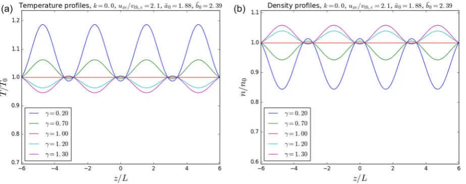
Provided the DF (24) is positive over the whole phase space, then the density, pressure, and temperature will also be positive everywhere. Note, however, that the opposite is not true, i.e., a positive density and pressure do not imply a positive DF. We ensure that the DF is positive by choosing parameters in such a way that the conditions (27) and(28) are satisfied (for both ions and electrons). Figure 1 shows profiles of the density and temperature for different values of

c, withk¼0 (the linear force-free case). Figure2shows the same quantities withk¼0.5. They are normalised to have a value of unity at the lowerz-boundary of each plot, and we have chosen parameters such that the DFs are positive for ions and electrons (note that if we chooseuxe=vth;e, then this

fixesuxi=vth;i through Eq. (A7), if we specify the mass ratio and the ratiobe=bi). Forc¼1:0 in each figure, we see that both the density and temperature are constant, as in Abraham-Shrauner’s model. For the other values ofcshown, the quantities have a periodic structure. In regions where the density is enhanced/depleted (with respect to the constant value forc¼1), there is a corresponding depletion/enhance-ment of the temperature, which ensures that the two quanti-ties multiply together to give a constant pressure, as required for the force-free equilibrium. Additionally, in regions where the values ofc>1 lead to an enhancement/depletion of the quantities, the opposite behaviour is seen whenc<1, i.e., a depletion/enhancement of the quantities. Similar features are seen by Kolotkov et al.2 (which we obtain in the limit

k!1), but note that the density and temperature are not periodic in this case, and so, for a particularcvalue, there is either an enhancement or depletion of the density/tempera-ture (not both).

We will now briefly discuss some other properties of the model. The plasma beta, defined in this case as the ratio of

Pzz to the magnetic pressure B20=ð2l0Þ, is given [using Eq.

(A11)] by

bpl¼

a0

c þb0þ

1

Using the conditions (27)and(28)for positivity of the DF, we have that

bpl> 1 2þ

1 2k2 exp

ck2u2xs 2v2

th;s !

ð1k2Þexp k

2_u2

ys 2v2

th;s ! 2

4

3 5:

(33)

For k¼0 and k¼1, for example, it is straightforward to show thatbplmust be greater than unity (as in, e.g., the

mod-els in Refs.1,2,38, and40), sinceu2xs=v

2

th;s0. The bulk-flow velocity components, defined by

Vs¼ 1

ns ð

vfsd3v; (34)

have the form

Vxs¼

cuxssnðz=LÞdnðz=LÞ

a0þb0þ1=2þðc1Þsn2ðz=LÞ

; (35)

Vys¼

uyscnðz=LÞdnðz=LÞ

a0þb0þ1=2þðc1Þsn2ðz=LÞ

; (36)

Vzs¼0: (37)

Through these expressions, we see the role played by the parametersuxsanduys, which can also be written in terms of

the ratio of the species gyroradius,rg;s, to the current sheet

half-width, L, by using Eq. (A16) (similarly to Neukirch

et al.39) as

u2

ys

v2

th;s ¼c

2_u2

xs

v2

th;s ¼4r

2

g;s

L2 : (38)

The current density can be calculated from the bulk flow velocity as

j¼X

s

qsnsVs; (39)

and has components

FIG. 2. (a) Density and (b) temperature profiles for various values ofc, fork¼0.5. Both quantities are normalised to have a value of unity at the lower z-boundary.

jx¼n0ecðuxiuxeÞsnðz=LÞdnðz=LÞ; (40)

jy¼n0eðuyiuyeÞcnðz=LÞdnðz=LÞ; (41)

jz¼0: (42)

Using Eqs.(A11)and(A17), we can show that these expres-sions are equivalent to those obtained macroscopically from Ampe`re’s law [Eq.(11)].

In the models in e.g., Refs. 1, 38, and 39, the spatial structure of the current density is determined solely by the structure of the bulk flow velocity since the density is con-stant, in contrast to the classic Harris sheet model,46where the bulk flow velocity is constant, and it is the spatial depen-dence of the density that determines the structure of the cur-rent density. In this extended model (and also that of Kolotkovet al.2), however, both the bulk-flow velocity and density are spatially dependent, and so the spatial structure of the current density is determined from the product of the two quantities.

A. Limiting values ofk

In the limitk!1, the number density, temperature, and pressure [Eqs. (29)–(31)] go to the form discussed by Kolotkovet al.2for the force-free Harris sheet, and the DF (24) becomes the Kolotkov DF (note that our notation is slightly different).

In the limit k!0, the field becomes linear force-free, and we get a DF of the form

fs¼

c3=2

n0expðcbsHsÞ ffiffiffiffiffiffi

2p

p

vth;s

3 a0

c2_u2

xs 4v2

th;s þc

4ðcbsuxspxspÞ

2

!

þ1 4

n0expðbsHsÞ ffiffiffiffiffiffi 2p

p

vth;s

3 4b02

u2

ys

v2

th;s

þbsuyspysþ2

2

!

;

(43)

which is a modified form of the DF obtained in the k!0 limit of the DF(14). The density and temperature have the form given by Eqs. (29) and (30), respectively, where snðz=LÞ ¼sinðz=LÞ.

V. VELOCITY SPACE STRUCTURE OF DF

In this section, we present some illustrative plots of the DF(24) to show the effect of changingc, i.e., the effect of changing the energy dependence of the different particle populations. In the vx- and vy- directions, it is possible to

choose sets of parameters for which there are multiple peaks in the DF, which may have implications for the stability of the equilibrium. Neukirch et al.39 and Abraham-Shrauner1 derive conditions on the parameters in their models such that their DFs will be single-peaked over the whole phase space. Due to the increased complexity of the DFs in terms of energy dependence, however, we have not yet carried out a full analysis of the velocity space structure—this is left for a future investigation.

In the discussion of the plots below, we will refer to the cases where the pxs population is “hotter”/“colder” than the pys one. This refers to thepxs population having an energy

dependence resulting in a “narrower”/“wider” Maxwellian factor in the DF than the pys one. We note, however, that

because the DFs are not purely Maxwellian, the temperature cannot be properly defined in terms of the width of the DF, but the widths of the first and second parts of the DF give us a qualitative measure of the temperature difference between the different populations. This notion of temperature should not be confused with the definition of the temperature given in Eq.(30).

A.vx-direction

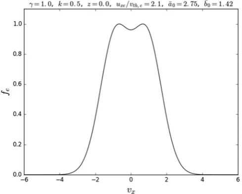
In Fig.3, we plot the electron DF(24)in thevx-direction

(for vy¼vz¼0) with c ¼ 1 (i.e., the Abraham-Shrauner DF). We have chosen a set of parameters for which, atz¼0, the DF has a double maximum in vx (these are the same

parameters as in Fig. 2). We note, however, that it is also possible to choose parameters for which the DF has only a single maximum in vx over the whole phase space, if

required (by increasing the density of the background popu-lations appropriately). In Fig.3, and all subsequent figures in this paper, we normalise the DF to have a maximum value of unity.

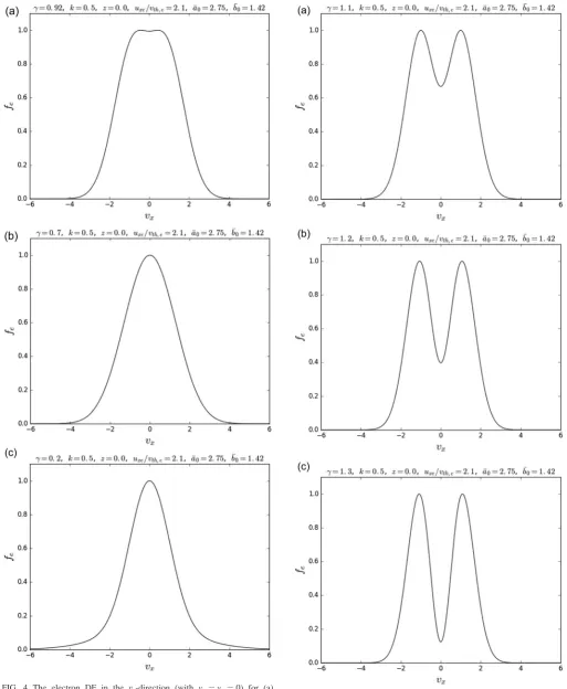
Our main aim in this section is to investigate the effect of changingcon the velocity space structure of the DF. This is why we have chosen parameters that give a double maxi-mum forc ¼ 1, since the effect of changingcis illustrated more clearly in such cases. Figure4shows plots of the elec-tron DF for various values ofcwhich are less than unity. For

c¼0:92, the double maximum still exists, but has become more slight; for the smaller values ofcshown (0.2 and 0.7), the double maximum has disappeared. In the vx-direction,

the second part of the DF (which does not depend onc) has the Maxwellian formgðpysÞexpðbsHsÞ. Forc<1, thepxs

-dependent population and the first background one are “hotter” than thepys-dependent and second background

pop-ulations, and so the Maxwellian factor expðcbsHsÞ(in the

first part of the DF) has a narrower width than the factor in the second part of the DF. The “narrow” first part of the DF, including the cosine which can give double maxima invx, is

therefore “swamped” by the wider second part for decreasing

c, and we see the behaviour in Fig.4.

Figure5shows plots of the electron DF for various val-ues ofc, which are greater than unity. We see that the double maximum in the middle becomes more pronounced as cis increased. This is due to the fact that the Maxwellian

FIG. 4. The electron DF in the vx-direction (with vy¼vz¼0) for (a)

c¼0:92, (b)c¼0:7, and (c)c¼0:2. _{FIG. 5. The electron DF in the v}

x-direction (with vy¼vz¼0) for (a)

expðcbsHsÞ multiplying the first part of the DF is now wider than the Maxwellian that multiplies the second part (the pxs-dependent population and the first background one

are now “colder” than the pys-dependent and second

back-ground populations), so the first part dominates and deter-mines the behaviour of the DF. In Figs.3–5, we have chosen the parametersa0 andb0 such that the DFs are positive for

all values ofcwe consider. As can be seen from the positiv-ity conditions(27), the minimum value ofa0becomes

signif-icantly larger ascis increased (for fixed values of the other parameters). If we were to further increasec, then the central “dip” of the DF would become more pronounced, and the DF would become negative; hence, we would need to increasea0(and adjustb0if required).

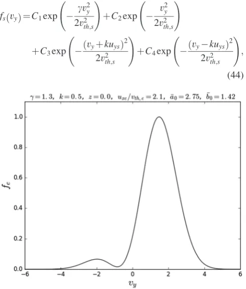
B.vy-direction

In this section, we will show some illustrative plots of the electron DF in the vy-direction for various values of c.

For the parameter set we used in Figs.3–5, the DFs are sin-gle peaked in all cases except for c¼1:3, where there is a double maximum as illustrated in Fig.6.

From initial investigations, it seems to be difficult to find a set of parameters from which we can illustrate the effect of increasing or decreasing c. This may be due to the fact that multiple maxima appear to occur at high values ofuxe=vth;e, for which we require large values ofa0to ensure positivity of

the DF—i.e., a large background density. This often results in the DF being single-peaked for smaller values ofc.

Possible behaviour of the DF in thevy-direction can be

explored heuristically by noting that, for given values vx,vz

andz, the DF has the general form

fsð Þ ¼vy C1exp

cv2

y 2v2

th;s !

þC2exp v2

y 2v2

th;s !

þC3exp

vyþkuys ð Þ2

2v2

th;s !

þC4exp

vykuys ð Þ2

2v2

th;s !

;

(44)

for constantsC1–C4, i.e., it consists of two Maxwellian parts with varying widths, and two shifted Maxwellians—one shifted in the positivevy-direction, and the other in the

nega-tive vy-direction (by the same amount). Depending on the FIG. 6. The electron DF in thevy-direction (withvx¼vz¼0) for the

param-eters used in Figure5(c).

relative values ofC1–C4, therefore, the DF can exhibit differ-ent behaviour, some examples of which are given in Fig.7. Note that we have taken different values ofa0 in each plot,

to ensure that the DFs are positive in each case.

VI. SUMMARY

In this paper, we have presented a class of 1D strictly neutral Vlasov-Maxwell equilibrium DFs for both linear and nonlinear force-free current sheets, with magnetic fields defined in terms of Jacobian elliptic functions, which are an extension of the DFs discussed by Abraham-Shrauner1 to account for non-uniformities in the temperature and density, whilst still maintaining a constant pressure (with respect to the spatial coordinate), as is required for force-balance of the force-free equilibrium. To achieve this, we have used the method of Kolotkov et al.,2 which involves modifying the DF of the original case to include temperature differences between the different particle populations in the model, and then ensuring that strict neutrality is satisfied and that there is consistency between the microscopic and macroscopic parameters of the equilibrium.

The new DF can be regarded as consisting of four parti-cle populations: one depending onpxs, one onpys, and two

background populations. The pxs-dependent and first

back-ground population are taken to have the same energy depen-dence in the DF, as do both the pys-dependent and second

background populations. Note that for the limit of vanishing elliptic modulus, k, to give continuous DFs and pressure, density, and temperature profiles, we require a particular choice of the constants characterising the background popu-lations, but this form can be changed for other kvalues if desired (it has the “drawback” of giving a very large maxi-mum density for certain parameter values).

We have derived sufficient conditions on the parameters such that the positivity of the DFs is ensured, and have given explicit expressions for the density, temperature, and pres-sure across the current sheet. Additionally, we have derived the components of the bulk-flow velocity from the DF, to show that the spatial structure of the current density is deter-mined by the product of the spatial structure of the density and bulk-flow velocity, in contrast to the models of, e.g., Abraham-Shrauner1and Neukirchet al.39where the current density structure is determined solely by the structure of the bulk-flow velocity, and also in contrast to the Harris sheet case,46where it is determined solely by the density structure. We have investigated limiting cases of the elliptic mod-ulus, k. Fork!1, the magnetic field becomes that of the force-free Harris sheet, and in this limit, we recover a DF similar to that found by Kolotkov et al.2 for this magnetic field. In the limitk!0, the magnetic field becomes linear force-free, and in Abraham-Shrauner’s case, the DF takes a form which is similar to the one discussed in Refs. 18,31, and37, but which is shifted inpxs andpys. In our extended

model, the k!0 limit simply gives an extension of this shifted DF to include non-uniformity in both the temperature and density.

We have also illustrated graphically the effect of chang-ing the temperature difference between the particle

populations in the DF. In the vx-direction, we found that

making the pxs part “colder” than the pys part can result in

rather pronounced double maxima of the DF (due to a cosine term invx), but when the pxspart is “hotter,” these maxima

are less significant, or the DF becomes single peaked. In the

vy-direction, the DF contains two drifting Maxwellians (with

the same energy dependence), and two non-drifting Maxwellians (with different energy dependences), and so there is the possibility of double maxima in the DF depend-ing on the relative values of the coefficients of the separate parts.

Double maxima in the DF may lead to velocity space instabilities (e.g., Ref. 47). Due to the increased complexity of the model, however, we have not attempted a systematic study of the velocity space structure, i.e., we have not derived conditions on the parameters such that the DF can be multi-peaked for some z, as has been done by Neukirch

et al.39 and Abraham-Shrauner.1 This is left for a future investigation. We note, however, that it will be possible to choose the density of the background populations large enough such that there are only single maxima of the DF over the whole phase space.

ACKNOWLEDGMENTS

We acknowledge the support of the Science and Technology Facilities Council via the consolidated Grant Nos. ST/K000950/1 and ST/N000609/1 and the doctoral training grant ST/K502327/1 (O.A.), and the Natural Environment Research Council via Grant No. NE/P017274/1 (Rad-Sat) (O.A.). F.W. and T.N. would also like to thank the University of St. Andrews for general financial support.

APPENDIX: PARAMETER RELATIONS

In Sec. IV, by imposing the strict neutrality condition

neðAx;AyÞ ¼niðAx;AyÞ ¼n, we obtain the relations

n0eexp

u2

xe 2v2

th;e !

¼n0iexp

u2

xi 2v2

th;i !

¼n0; (A1)

a0eexp

u2

xe 2v2

th;e !

¼a0iexp

u2

xi 2v2

th;i !

¼a0; (A2)

a1eexp 1þck2

u2

xe 2v2

th;e !

¼a1iexp 1þck2

u2

xi 2v2

th;i !

¼a1;

(A3)

b0eexp

u2

xe 2v2

th;e !

¼b0iexp

u2

xi 2v2

th;i !

¼b0: (A4)

b1eexp

k2_u2

yeu2xe 2v2

th;e !

¼b1iexp

k2_u2

yiu2xi 2v2

th;i !

¼b1; (A5)

b2eexp

k2_u2

yeu2xe 2v2

th;e !

¼b2iexp

k2_u2

yiu2xi 2v2

th;i !

¼b2; (A6)

beuye¼biuyi: (A8)

Using the choices (20)and (21) for a0s andb0s, the

condi-tions(A2)and(A4)can equivalently be written as

a0eexp

u2

xe 2v2

th;e !

¼a0iexp

u2

xi 2v2

th;i !

¼a0; (A9)

b0eexp

u2xe 2v2

th;e !

¼b0iexp

u2xi 2v2

th;i !

¼b0; (A10)

wherea0¼a0þc=ð2k2Þ;b0¼b01=ð2k2Þ.

By calculating two expressions for the pressure Pzz, in

terms of the macroscopic and microscopic parameters of the equilibrium, respectively, and comparing these expressions, we obtain the relations

n0

beþbi

bebi ¼ B

2 0

2l0

; (A11)

a0

c þb0¼

Pt1þPt2 B2

0=2l0

3

2; (A12)

a1

c ¼

1

2k2; (A13)

b1¼

1 4

1

kþ1

2

; (A14)

b2¼

1 4

1

k1

2

; (A15)

2

B0L

¼cbsjuxsjqs¼bsuysqs)uys¼cjuxsj: (A16)

Similarly to previous work (e.g., Ref.39), we can derive an expression for the current sheet half-widthL, in terms of the microscopic parameters, as

L¼ 2ðbeþbiÞ

l0e2bebin0ðuyiuyeÞ2 !1=2

: (A17)

1

B. Abraham-Shrauner, “Force-free Jacobian equilibria for Vlasov-Maxwell plasmas,”Phys. Plasmas20(10), 102117 (2013).

2

D. Y. Kolotkov, I. Y. Vasko, and V. M. Nakariakov, “Kinetic model of force-free current sheets with non-uniform temperature,” Phys. Plasmas

22(11), 112902 (2015).

3_{N. A. Bobrova and S. I. Syrovatskii, “Violent instability of}

one-dimensional forceless magnetic field in a rarefied plasma,” Sov. J. Exp. Theor. Phys. Lett.30, 535 (1979).

4

M. G. Kivelson and K. K. Khurana, “Models of flux ropes embedded in a Harris neutral sheet: Force-free solutions in low and high beta plasmas,” J. Geophys. Res.100, 23637–23646, doi:10.1029/95JA01548 (1995). 5

G. E. Marsh, Force-Free Magnetic Fields: Solutions, Topology and Applications(World Scientific, Singapore, 1996).

6

E. Tassi, F. Pegoraro, and G. Cicogna, “Solutions and symmetries of force-free magnetic fields,”Phys. Plasmas15(9), 092113 (2008). 7

E. V. Panov, A. V. Artemyev, R. Nakamura, and W. Baumjohann, “Two types of tangential magnetopause current sheets: Cluster observations and theory,” J. Geophys. Res. (Space Phys.) 116, A12204, doi:10.1029/ 2011JA016860 (2011).

8

T. Wiegelmann and T. Sakurai, “Solar force-free magnetic fields,”Living Rev. Sol. Phys.9(1), 5 (2012); ISSN 1614-4961.

9

P. Eric,Magnetohydrodynamics of the Sun(Cambridge University Press, 2014).

10_{I. Y. Vasko, A. V. Artemyev, A. A. Petrukovich, and H. V. Malova, “Thin}

current sheets with strong bell-shape guide field: Cluster observations and models with beams,”Ann. Geophys.32, 1349–1360 (2014).

11

L. M. Zelenyi, A. G. Frank, A. V. Artemyev, A. A. Petrukovich, and R. Nakamura, “Formation of sub-ion scale filamentary force-free structures in the vicinity of reconnection region,”Plasma Phys. Controlled Fusion

58(5), 054002 (2016).

12_{C. Akcay, W. Daughton, V. S. Lukin, and Y.-H. Liu, “A two-fluid study of}

oblique tearing modes in a force-free current sheet,”Phys. Plasmas23(1), 012112 (2016).

13_{D. Burgess, P. W. Gingell, and L. Matteini, “Multiple current sheet systems}

in the outer heliosphere: Energy release and turbulence,”Astrophys. J.822, 38 (2016).

14_{A. V. Artemyev, V. Angelopoulos, J. S. Halekas, A. Runov, L. M.}

Zelenyi, and J. P. McFadden, “Mars’s magnetotail: Nature’s current sheet laboratory,”J. Geophys. Res.: Space Phys.122, 5404–5417, doi:10.1002/ 2017JA024078 (2017); ISSN 2169-9402.J.

15

A. V. Artemyev, V. Angelopoulos, J. Liu, and A. Runov, “Electron cur-rents supporting the near-Earth magnetotail during current sheet thinning,” Geophys. Res. Lett.44, 5–11, doi:10.1002/2016GL072011 (2017). 16

Reconnection of Magnetic Fields: Magnetohydrodynamics and Collisionless Theory and Observations, 1st ed., edited by J. Birn and E. R. Priest (Cambridge University Press, 2007), p. 3, ISBN 9780521854207. 17

F. Wilson, T. Neukirch, M. Hesse, M. G. Harrison, and C. R. Stark, “Particle-in-cell simulations of collisionless magnetic reconnection with a non-uniform guide field,”Phys. Plasmas23(3), 032302 (2016).

18

M. G. Harrison and T. Neukirch, “Some remarks on one-dimensional force-free Vlasov-Maxwell equilibria,” Phys. Plasmas 16(2), 022106 (2009).

19

M. Hesse, M. Kuznetsova, K. Schindler, and J. Birn, “Three-dimensional modeling of electron quasiviscous dissipation in guide-field magnetic reconnection,”Phys. Plasmas12(10), 100704 (2005).

20

Y.-H. Liu, W. Daughton, H. Karimabadi, H. Li, and V. Roytershteyn, “Bifurcated structure of the electron diffusion region in three-dimensional magnetic reconnection,”Phys. Rev. Lett.110, 265004 (2013).

21

F. Guo, H. Li, W. Daughton, and Y.-H. Liu, “Formation of hard power laws in the energetic particle spectra resulting from relativistic magnetic reconnection,”Phys. Rev. Lett.113, 155005 (2014).

22

F. Guo, Y.-H. Liu, W. Daughton, and H. Li, “Particle acceleration and plasma dynamics during magnetic reconnection in the magnetically domi-nated regime,”Astrophys. J.806, 167 (2015).

23

F. Zhou, C. Huang, Q. Lu, J. Xie, and S. Wang, “The evolution of the ion diffusion region during collisionless magnetic reconnection in a force-free current sheet,”Phys. Plasmas22(9), 092110 (2015).

24

F. Guo, X. Li, H. Li, W. Daughton, B. Zhang, N. Lloyd-Ronning, Y.-H. Liu, H. Zhang, and W. Deng, “Efficient production of high-energy non-thermal particles during magnetic reconnection in a magnetically domi-nated ion-electron plasma,”Astrophys. J. Lett.818, L9 (2016).

25_{F. Guo, H. Li, W. Daughton, X. Li, and Y.-H. Liu, “Particle acceleration}

during magnetic reconnection in a low-beta pair plasma,”Phys. Plasmas

23(5), 055708 (2016). 26

F. Fan, C. Huang, Q. Lu, J. Xie, and S. Wang, “The structures of magnetic islands formed during collisionless magnetic reconnections in a force-free current sheet,”Phys. Plasmas23(11), 112106 (2016).

27

N. A. Bobrova, S. V. Bulanov, J. I. Sakai, and D. Sugiyama, “Force-free equilibria and reconnection of the magnetic field lines in collisionless plasma configurations,”Phys. Plasmas8, 759–768 (2001).

28

K. Nishimura, S. P. Gary, H. Li, and S. A. Colgate, “Magnetic reconnec-tion in a force-free plasma: Simulareconnec-tions of micro- and macroinstabilities,” Phys. Plasmas10, 347–356 (2003).

29

K. Bowers and H. Li, “Spectral energy transfer and dissipation of magnetic energy from fluid to kinetic scales,”Phys. Rev. Lett.98(3), 035002 (2007). 30

W. Alpers, “Steady state charge neutral models of the magnetopause,” Astrophys. Space Sci.5, 425–437 (1969).

31_{P. J. Channell, “Exact Vlasov-Maxwell equilibria with sheared magnetic}

fields,”Phys. Fluids19, 1541–1545 (1976). 32

F. Mottez, “Exact nonlinear analytic Vlasov-Maxwell tangential equilibria with arbitrary density and temperature profiles,” Phys. Plasmas 10, 2501–2508 (2003).

33

34

E. Moratz and E. W. Richter, “Elektronen-Geschwindigkeitsverteil ungsfunktionen f€ur kraftfreie bzw. teilweise kraftfreie Magnetfelder,”Z. Naturforsch., A21, 1963 (1966).

35_{A. Sestero, “Self-consistent description of a warm stationary plasma in a}

uniformly sheared magnetic field,”Phys. Fluids10, 193–197 (1967). 36

D. Correa-Restrepo and D. Pfirsch, “Negative-energy waves in an inhomo-geneous force-free Vlasov plasma with sheared magnetic field,” Phys. Rev. E47, 545–563 (1993).

37_{N. Attico and F. Pegoraro, “Periodic equilibria of the Vlasov-Maxwell}

sys-tem,”Phys. Plasmas6, 767–770 (1999). 38

M. G. Harrison and T. Neukirch, “One-dimensional Vlasov-Maxwell equi-librium for the force-free Harris sheet,”Phys. Rev. Lett.102(13), 135003 (2009).

39

T. Neukirch, F. Wilson, and M. G. Harrison, “A detailed investigation of the properties of a Vlasov-Maxwell equilibrium for the force-free Harris sheet,”Phys. Plasmas16(12), 122102 (2009).

40_{F. Wilson and T. Neukirch, “A family of one-dimensional}

Vlasov-Maxwell equilibria for the force-free Harris sheet,” Phys. Plasmas 18, 082108 (2011).

41

C. R. Stark and T. Neukirch, “Collisionless distribution function for the relativistic force-free Harris sheet,”Phys. Plasmas19(1), 012115 (2012). 42

O. Allanson, T. Neukirch, F. Wilson, and S. Troscheit, “An exact colli-sionless equilibrium for the Force-Free Harris Sheet with low plasma beta,”Phys. Plasmas22(10), 102116 (2015).

43

D. Nicolas, B. Gerard, A. Nicolas, D. Jeremy, and R. Laurence, “Asymmetric kinetic equilibria: Generalization of the bas model for rotat-ing magnetic profile and non-zero electric field,” Phys. Plasmas22(9), 092904 (2015).

44

NIST Digital Library of Mathematical Functions, edited by F. W. J. Olver, A. B. Olde Daalhuis, D. W. Lozier, B. I. Schneider, R. F. Boisvert, C. W. Clark, B. R. Miller, and B. V. Saunders (DLMF, 2016).

45_{P. F. Byrd and M. David Friedman,Handbook of Elliptic Integrals for}

Engineers and Scientists(Springer, Berlin, 2013). 46

E. G. Harris, “On a plasma sheath separating regions of oppositely directed magnetic field,”Nuovo Cimento23, 115 (1962).

47_{S. Peter Gary, Theory of Space Plasma Microinstabilities, Cambridge}