Exploiting orientation selective DEER : determining molecular structure in systems containing Cu(II) centres

(1)

Cite this:Phys. Chem. Chem. Phys., 2016,18, 5981

Exploiting orientation-selective DEER: determining

molecular structure in systems containing Cu(

II

)

centres

†

Alice M. Bowen,‡abMichael W. Jones,‡aJanet E. Lovett,acThembanikosi G. Gaule,d

Michael J. McPherson,d Jonathan R. Dilworth,aChristiane R. Timmel*aand

Jeﬀrey R. Harmer*ae

Orientation-selective DEER (Double Electron-Electron Resonance) measurements were conducted on a series of rigid and flexible molecules containing Cu(II) ions. A system with two rigidly held Cu(II) ions was

aﬀorded by the protein homo-dimer of copper amine oxidase from Arthrobacter globiformis. This system provided experimental DEER data between two Cu(II) ions with a well-defined distance and

relative orientation to assess the accuracy of the methodology. Evaluation of orientation-selective DEER (os DEER) on systems with limited flexibility was probed using a series of porphyrin-based Cu(II)–nitroxide

and Cu(II)–Cu(II) model systems of well-defined lengths synthesized for this project. Density functional theory was employed to generate molecular models of the conformers for each porphyrin-based Cu(II) dimer studied. Excellent agreement was found between DEER traces simulated using these computed conformers and the experimental data. The performance of different parameterised structural models in simulating the experimental DEER data was also investigated. The results of this analysis demonstrate the degree to which the DEER data define the relative orientation of the two Cu(II) ions and highlight the need to choose a parameterised model that captures the essential features of the flexibility (rotational freedom) of the system being studied.

Introduction

Pulse dipolar spectroscopy (PDS) is a powerful technique providing structural information in biological and materials sciences applications by measurement of the distance (from ca.1.5 to 8 nm for protonated systems andZ10 nm in deuterated systems)1,2and, in favourable cases, orientations between two

paramagnetic spin probes. As the majority of biomolecules are naturally diamagnetic, PDS studies on such systems typically employ spin labels, for example the nitroxide MTSL (S-(2,2,5,5- tetramethyl-2,5-dihydro-1H-pyrrol-3-yl)methylmethanesulfono-thioate) which can be attached selectively to the protein of interest through site directed spin labelling of a targeted cysteine residue and formation of a covalent disulfide linkage.3

The results of PDS report directly on the inter-spin dipolar interaction, from which a distance distribution can be easily computed for experiments without orientational selection using Tikhonov regularization.4The distance distribution obtained can yield information on the flexibility of the spin label tether and/or any structural disorder in the molecule.5,6However, at the typically employed X- and Q-band frequencies, the inherent flexibility of the MTSL tethers often results in a loss of all inter-spin orientation information.7_{Although orientation selection may complicate the}

analysis, its presence can provide a wealth of additional informa-tion about the molecular system if it can be successfully measured and modelled.8–10

Intrinsic paramagnetic centres in biomolecules are, in principle, ideal spin probes to be exploited in a PDS experiment.11,12They are usually fixed rigidly within their parent biomolecule resulting in very accurate and narrow inter-spin distance distributions. a_{Centre for Advanced Electron Spin Resonance, University of Oxford, South Parks}

Road, Oxford, OX1 3QR, UK. E-mail: [email protected] b_{Institute of Physical and Theoretical Chemistry, Goethe University Frankfurt,}

Max-von-Laue-Str. 7, 60438, Frankfurt am Main, Germany

c_{SUPA, School of Physics and Astronomy, University of St Andrews, North Haugh,}

St Andrews, KY16 9SS, UK d

Astbury Centre for Structural Molecular Biology, Institute of Molecular and Cellular Biology, Faculty of Biological Sciences, University of Leeds, Leeds LS2 9JT, UK

e_{Centre for Advanced Imaging, University of Queensland, St Lucia, QLD, 4072,}

Australia. E-mail: Jeﬀ[email protected]

†Electronic supplementary information (ESI) available: Detailed synthetic schemes, procedures and characterization data for the compounds studied. CCDC 1040894. For ESI and crystallographic data in CIF or other electronic format see DOI: 10.1039/c5cp06096f

‡A. M. B. (ESR measurements and analysis) and M. W. J. (Model system synthesis) contributed equally.

Received 9th October 2015, Accepted 15th December 2015

DOI: 10.1039/c5cp06096f

www.rsc.org/pccp

PAPER

Open Access Article. Published on 03 February 2016. Downloaded on 11/03/2016 13:49:10.

This article is licensed under a

Creative Commons Attribution 3.0 Unported Licence.

View Article Online

(2)

Conversely, significant flexibility and/or disorder of the protein structure (e.g.unfolded proteins or diﬀerent conformations) will dominate the distance distribution profile allowing assessment and quantification of these factors. Intrinsic Cu(II) centres

con-stitute important spin probes for PDS as they occur widely in biology; for example in hemocyanin, laccases, superoxide dis-mutases and ceruloplasmin. Many biomolecules contain other naturally occurring metal cations, e.g.zinc (found in the zinc finger domains of many DNA binding proteins), iron (present in the plethora of heme containing proteins) or manganese (occurring in Arginase, a member of the ureohydrolase family of enzymes). Whilst many of these metal cations are paramagnetic themselves, their replacement by Cu(II),13if chemically feasible,

would be advantageous as its relatively long relaxation times and low g-value anisotropy make it a suitable candidate for PDS studies. Biologically copper is important, for example the binding of Cu(II) to amyloid-beta fibrils of Alzheimer’s disease has also been observed.14Copper centres have recently been incorporated into the helix of DNA using tailored metal mediated base pairs, providing a rigid spin probe for potential PDS spectroscopy studies.15–18_{Furthermore, copper has been incorporated into a}

protein structure in the form of a copper binding loop and distances between this centre and a nitroxide spin label probed using both DEER (Double Electron Electron Resonance), synony-mously PELDOR (Pulsed Electron Double Resonance), and relaxa-tion measurements.19 It has also been shown that in some proteins copper can associate selectively with histidine residues, allowing the inter-residue distance to be used to identify the site of interaction.20Based upon this, a bis-histidine moiety has been designed as a selective binding site for copper and been shown to provide a stable copper based spin label for DEER experiments.21 Alternatively a cysteine specific copper tag has been synthesised, that can be attached to the proteinviaa disulfide linkage in a similar manner to the nitroxide MTSL mentioned previously.22

Here we study molecules containing Cu(II) centres with

orientation selective PDS experiments using three and four-pulse DEER. The orientation selectivity is a result of the microwave pulses exciting only a small part of the Cu(II) EPR spectrum:

at X-band (B9.5 GHz), the Cu(II) spectrum extends over some

500 MHz due tog-anisotropy and the copper hyperfine couplings whilst the bandwidth of a typicalp/2 pulse (e.g., 16 ns) does not exceed 50 MHz. This selectivity of the microwave (mw) pulse results in a particular DEER experiment only exciting a relatively small set of molecular orientations of the pair of Cu(II) spins

(inter-spin vectors) with respect to the magnetic field vector,B0.

To date there have been several DEER reports using Cu(II) ions. The first such study was carried out on a homo-dimer of the protein Azurin by van Amsterdamet al.11who extracted an approximate distance but no orientation information. Cu(II)–

Cu(II) distances were also measured in a protein (multi-copper

nitrate reductase) by van Wonderen et al.23 who applied a relaxation filter to distinguish between different copper centres, however their study did not account for orientation effects. More recently, Merzet al.24measured inter-copper distances in Superoxide Dismutase (SOD1) using both DEER and 6-pulse Double Quantum Coherence (DQC) at Ku-band (17 GHz).

Although orientation selection was considered, the effect was determined to be small due to the relative orientation of the two copper centres and no account was made of this in the analysis. Orientation selection was also observed although not analysed by Narret al.25_{on a copper bisnitroxide model system. The first}

orientation-selective DEER analysis study on Cu(II)–NOmodel

systems was presented by Bodeet al.26,27who used a geometric model, based on a 151bend of the linker and rotation of the nitroxide moiety around this linker, as the basis for their simula-tions. The use of the nitroxide moiety significantly simplified the orientational analysis as only the Cu(II) orientational selection

needed to be considered. The orientation selection between a Cu(II)–nitroxide spin pair was also considered by Abdullinet al.28

who used this information to allow for the trilateration of the position of the bound copper ion within a monomer of Azurin that had been labelled with MTSL nitroxide at known positions. Saxenaet al.29–32studied two Cu(II) centres each coordinated by the hexapeptide sequence PHGGGW which is implicated in a number of prion diseases,33–35_{with each copper moiety linked}

by a number of proline amino acids (PHGGGW(P)nHGGGW, with variablen). The initial system, PHGGGWPPPHGGGW with Cu(II)

coordinated, did not show any orientation selectivity due to the system geometry.29Using a chemically similar but geometrically different model system (PHGGGWPPPPPHGGGW) the same authors were able to perform an orientational analysis of two copper centres using a generic molecular model,20,30,31which may not be applicable in all circumstances, as discussed below. Marko et al.36,37discussed a model free approach using data from rigid bisnitroxide systems fitted using a simulated DEER trace library to reconstruct the experimental data. However, the symmetry of the spin system prevented determination of a unique solution. Currently no universal single method exists for the analysis of orientation-selective DEER with a distribu-tion of spin–spin distances and orientadistribu-tions and consequently best results rely on some prior structure knowledge to reduce the number of possible solution sets.

The aim of this study is to explore the limits and capabilities of orientation-selective DEER in extracting distance and orien-tation information from systems containing two Cu(II) spins.

Firstly, we investigated the homo-dimer of copper amine oxidase fromArthrobacter globiformis, a protein system embedding two tightly coordinated Cu(II) centres well characterized by high

quality X-ray data. Next we examined a series of porphyrin-based Cu(II)–Cu(II) rod-like molecules of differing lengths with a

reasonably large degree of conformational flexibility and, in addition, the corresponding Cu(II)–NOand NO–NOsystems. Different models were analysed with regard to their capability of describing the conformational flexibility and the resulting orientation-selective DEER traces.

Experimental

Experimental synthesis

The model compounds were designed to be semi-rigid rods holding the two radical labels a fixed distance apart. Cu(II)–Cu(II) (1–5),

(3)

Cu(II)–NO(6and7) and bisnitroxide, NO–NO(8), derivatives

were prepared by multi-step synthesis to provide benchmark measurements against which the accuracy of the modelling could be reliably ascertained. The stability and convenient synthesis and purification routes of the tetraphenyl porphyrin template made it the obvious choice of copper-chelating moiety for this study. Attempts to use several other well-known Cu(II)

ligands were not successful due to the formation of polymeric material during coordination to Cu(II) under a range of

condi-tions. The amide functionality acts as a type of ‘circuit breaker’ diminishing the through-bond electronic exchange that could occur between the two paramagnetic centres impeding the determination of accurate distances. To minimize the level of uncertainty in the spin–spin distances and orientations, the central spacers were designed to be as stable and rigid as possible. However, the DFT calculations (below) show that the molecules still exhibit a significant angular flexibility.

The target molecules were prepared by the peptide coupling of 5-(4-aminophenyl)-10,15,20-triphenylporphyrin (TPPNH2)38,39

or 4-amino-TEMPO with the requisite 1,4-phenyl dicarboxylic acids, and subsequent metallation with Cu(II). With the

excep-tion of terephthalic acid which was commercially available and 1,1-biphenyl-4,40_{-dicarboxylic acid (available as the diester), the} diacids containing 3–5 phenyl groups in the central linkers were prepared with Suzuki coupling reactions and subsequent ester hydrolysis. Polyaromatic molecules often suffer from solubility problems which can be circumvented by the attachment of aliphatic sidegroups, as for instance employed by Godtet al.40in the synthesis of model bisnitroxides for use in their DEER methodology work. For compounds with three or more phenyl groups in the central linker it was necessary to employ this strategy. The two smaller compounds, with 1- and 2-phenyl groups as the central spacer, did not suffer from significant solubility problems. BOP (benzotriazol-1-yloxytris(dimethylamino)-phosphonium hexafluorophosphate) coupling with an excess of the TPPNH2congener in all cases afforded the diporphyrin proligands

in moderate yields after flash chromatography. Metallation of the diporphyrin species was relatively trivial; a methanolic solution of Cu(II) acetate was introduced to a stirred solution of diporphyrin in

chloroform and the subsequent mixture heated at reflux to afford the model compounds1–5cleanly.

The Cu(II)–NOspecies6and7were preparedviathe BOP

coupling of one equivalent of TPPNH2to the requisite acid, followed

by attachment of the TEMPO motif also using a BOP mediated coupling procedure. This order of addition was employed to aid purification processes as the porphyrin derivative is clearly visible (dark purple) on silica gel. Finally, the insertion of metal was achieved in the same way as for the symmetrical Cu(II)–Cu(II) species. The NO_–NO _compound₈ _{was prepared simply, again by BOP} mediated coupling of the TEMPO–NH2motif to the 3-phenyl acid.

The compounds were characterized (where appropriate) by thin layer chromatography and MALDI analysis, UV-vis and IR spectroscopy,

1_{H and}13_{C NMR, mass spectrometry and CW-EPR at X-band.}

Detailed synthetic schemes and relevant characterization data for all of the compounds prepared and the intermediates are given in the ESI.†

Sample preparation

Samples of Cu(II)–Cu(II), Cu(II)–NOand NO–NOmodel systems

(compounds1–8) were prepared to a concentration of 0.1 mM in a 1 : 1 : 1 mixture of chloroform : toluene : THF. Toluene was included to preventp-stacking of aromatic rings of the compounds and a chloroform/THF mixture was found to form a suitable frozen glass. To account for the different relaxation properties of Cu(II) and

nitroxides, EPR measurements on the Cu(II)–Cu(II) systems (1–5)

were conducted at 15 K, those on the Cu(II)–NOsystems (6and7)

at 25 K and those on the NO–NO (8) system at 50 K. These temperatures were chosen as they provided the most favourable combinations of T1andT2.

Recombinant copper amine oxidase from A. globiformis (AGAO) with a C-terminal Strep-tag II, was prepared inE. coli according to the method of Judaet al.41A stock solution of strep-tagged copper amine oxidase was prepared using 120 mg ml1

(1.7 mM concentration of the protein monomer) in 50 mM HEPES buﬀer at pH 7.2. This stock solution was diluted, adding 30% glycerol by volume to produce the EPR sample containing ca.1.2 mM concentration of the protein monomer. EPR measure-ments on this system were also conducted at 15 K.

DEER spectroscopy

Experiments were recorded at X-band on a Bruker Elexsys E680 pulsed spectrometer equipped with an Oxford Instruments cryostat using a 3 mm split-ring Bruker resonator (EN 4118X-MS3). DEER experiments with Cu(II)–NOand NO–NOcentres

used a four-pulse (4P) DEER sequence1,42witht₂times of 1ms and 2ms for the 1-phenyl (6) and 3-phenyl (7) Cu(II)–NOsystems,

respectively and 0.8ms for NO_–NO₍₈_{). The short phase memory} times of the Cu(II)–Cu(II) and AGAO samples necessitated the

use of the simpler three-pulse (3P) DEER sequence43,44to collect traces of sufficient length such that oscillations could be observed. 3P DEER traces have a dead-time resulting from pulse overlap which obscures the zero-time. Therefore 3P DEER was collected with attime of 1500 ns (Cu(II)–Cu(II) systems, compounds1–5)

and 2000 ns (AGAO), and 4P DEER with at2= 200 ns. The 3P

and 4P traces were then combined using DEER-Stitch.45For all experiments thep/2 andp observer pulses were 32 ns with a 12 ns pump pulse.

Analysis methods

Orientation selective DEER

Our DEER trace simulation algorithm is described in detail elsewhere.10Briefly, the time-domain trace for intra-molecular interaction between pairs of spins is described by

F(t) = 1D(1f(t)) (1)

whereD is the modulation depth and f(t) the reduced form factor,46both of which depend upon the positions and excita-tion profiles of the microwave (mw) pulses and hence describe the orientation selection. The DEER trace simulation algorithm computes bothf(t) andD. The accuracy off(t) is suﬃcient such that no adjustment is required. However, the modulation depth,D,

(4)

is sensitive to experimental settings such as the p pulse flip angle, the resonator bandwidth, the inhomogeneity of the excitation mw fieldB1over the sample volume as well as the

degree of paramagnetic labelling. Consequently our simulated modulation depth,D_sim, was not accurate enough to describe the experimental traces. Therefore, a fitted scaling factor,c, was used to account for these modelling deficiencies such that

D=cD_sim (2)

Note that parameter,c, should be constant for all DEER traces from a given sample recorded under identical tuning condi-tions. If a simulation is conducted using the same pulse lengths as employed in the collection of the experimental data set, then c r 1 as in the simulations the pulse excitation bandwidth exceeds the experimental one (because of the resonator band-width and non-ideal pulse shapes and B1 profiles), and we

assume a labelling eﬃciency of 100%. The experimental DEER trace, D(t), is the product of intra-molecular, F(t), and inter-molecular (background)B(t), contributions:

D(t) =F(t)B(t) (3)

As the molecules studied here form a homogenous distribution of randomly orientated spins when frozen in a glassy matrix, the background function is given byB(t) = exp(kt).kis a function of spin concentration, however, as the local spin concentration was not known independently,k is treated here as a fitting para-meter. Further details of the DEER simulation methodology are given in the ESI.†

Modelling the conformations of the porphyrin-based rod-like model systems

To compute the reduced form factor f(t) starting from first principles requires knowledge of the molecular conformations and their corresponding relative populations. Our approach to determine the conformation ensemble of each molecule used density functional theory (DFT) calculations. For this we employed the Amsterdam Density Functional (ADF)47,48software package with a BLYP functional and a TZ2P basis set.

The molecules (Fig. 1) are relatively large for DFT geometry optimizations and exhibit a large number of torsional angles resulting in slow convergence of the geometry optimization. To overcome this and reduce calculation time we assumed that rotation about each flexible bond is independent of rotation about all other flexible bonds within the molecule. This allowed each molecule to be broken down into smaller molecular frag-ments (see ESI†for details for the fragments used). By calculat-ing a linear transit for the rotation of each flexible bond within a fragment and optimizing the geometry at 101 intervals an energy profile for the rotation about the bond was computed. All angles found withinkBTat the freezing point of the solvent

(kB= 8.6173105eV K1, Boltzmann constant,T= 134.15 K,

kBT= 0.11547 eV) were assumed to be thermally accessible and

equally populated, thus providing an allowed range of torsion angles for each bond type. A Monte Carlo approach to deter-mine a set of molecular configurations was then obtained by rotating each of the flexible bonds of each fragment by a randomly selected angle that lies within the calculated allowed range of torsion angles for that bond type. Plots of the energy

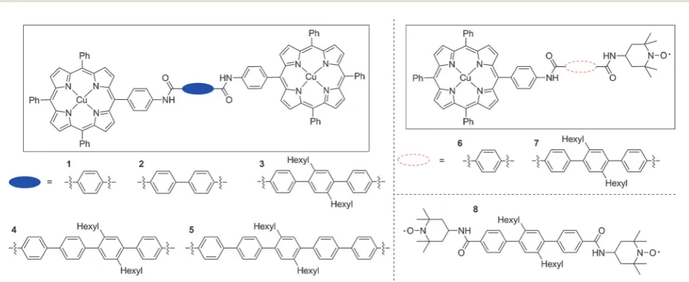
Fig. 1 The chemical structures of the model compounds synthesised and studied in this paper. For the DFT derived model 1 and the related model 2 (see

below), rigid rods were defined about which rotation could occur to describe the relative positions of the two spin centres. For the compounds1–5, in both porphyrin moieties a rod was defined as running from the copper to the closest amide nitrogen, and in the centre of the molecule a rod was defined as running along the length of the bridging linker between the amide carbonyl carbons. In compounds6and7similar rods were defined for the porphyrin moiety and the central linker. At the nitroxide, a rod was defined to run along the bond between the amide nitrogen and the carbon of the six member ring. The nitroxide spin density was localised to the oxygen and the relative angle of the vector linking this atom to the end of the rod between the amide nitrogen and the carbon in the ring was fixed, however rotation was allowed around this rod. Compound8used the same definition of the rod between the amide bond and the nitroxide moiety described above for both nitroxides and also a rod linking the two carbonyl carbons along the central linker.

[image:4.595.53.546.418.620.2]

(5)

profiles for each of the bonds and the distribution profiles of the two Cu(II) ions with respect to each other for each molecule are given in the ESI†(Fig. S2).

Spin density distribution

An important parameter required for the simulation of DEER time traces is the location of the spin density, r. The DFT calculation for the Cu(II)–porphyrin molecular fragment yielded a

spin density distribution withr(Cu) = 51%, and on each nitrogen r(N) = 11%. This result is similar to that calculated by Bodeet al. (r(Cu) = 56%, r(N) = 10.6%).27 _{However, it is known that DFT}

calculations frequently overestimate covalent bonding for the Cu(II) ion, resulting in too much spin transfer onto the ligands.49

A previously employed model for the copper porphyrin moiety used r(Cu) = 84% and r(N) = 4%,10 which is consistent with typical porphyrin nitrogen hyperfine couplings. Given this uncer-tainty, it was therefore decided to test the sensitivity of the DEER simulations to changes in the spin density distribution between the Cu(II) ion and the coordinating nitrogens (see below).

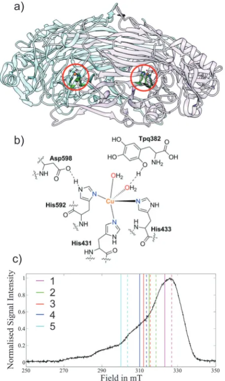
A. globiformis Amine Oxidase (AGAO) contains a copper centre ligated by three histidine ligands and two water molecules, one equatorial and the other axial, as shown in Fig. 2b. DFT studies on the isolated reaction centre fromHansenula polymorpha copper amine oxidase, which is structurally very similar to AGAO have been published previously.50In these calculations r(Cu)D62% andr(N) = 11% (the remainder of the spin density was delocalised over the rest of the porphyrin). These results are comparable to the DFT data calculated for the copper– porphyrin systems where again the degree of covalent bonding is likely to be overestimated. In the DEER simulations for AGAO we tested three distributions withr(N) = 0%, 5% and 10% with the remaining spin density on the Cu(II) ion,r(Cu) = 100%, 85%

and 70%, respectively. A different DEER response is theoretically expected with a change in the spin density distribution because the dipolar frequency scales as 1/r3. Comparing the results from all three trials no significant difference was observed in the DEER traces calculated, which results from the small region over which the spin density is distributed as compared to the relatively large inter-copper distance.

For the nitroxide, the spin density is essentially split between the nitrogen and the oxygen, with the larger portion localised on the oxygen.51_{In all the following calculations the}_r_{was positioned}

wholly on the oxygen,r(O) = 100%.

Results and discussion

Cu(II) centres with a single fixed orientation

The two Cu(II) centres in the protein homodimer of AGAO

(Fig. 2a) are separated by a well-defined distance and related by one single relative orientation as characterized by a number of X-ray studies. The protein therefore serves as an ideal model system to test the accuracy of orientation-selective DEER on Cu(II) containing molecules. Fig. 2c shows the observer

posi-tions for the five orientation-selective DEER measurements which were carried out.

The crystal structure (pdb code: 1IU7)52provides the relative orientations of the two Cu(II) centres with respect to one

another. However, it does not provide direct information on theg-tensor orientations of the two centres with respect to the molecular frame.

Experimental single-crystal studies for a copper tetraphenyl porphyrin centre, in which the copper centre is ligated by four nitrogens, have shown that theg-tensor is aligned such that the gzaxis is perpendicular to the plane of the porphyrin ring.53In comparison the distorted geometry of the AGAO copper centre (Fig. 2b), in which the copper is ligated by three histidines and two water molecules in our aerobic preparation52(in anaerobic preparations the oxygen of tyrosine 382 replaces the water)54 makes predicting the g-tensor orientation more complex. A DFT study performed on a phenolate Cu(II) compound,55

Fig. 2 (a) X-ray structure of the Copper Amine Oxidase (AGAO) homodimer

(pdb code: 1IU7)52_from_{A. globiformis}_{with the Cu(}

II) centres highlighted in red circles. (b) Cu(II) coordination sphere showing the histidine residues and water molecules. (c) Field-sweep X-band EPR spectrum depicting the DEER pulse positions; experiments are grouped in coloured pairs with dashed lines representing pump positions and solid lines detection positions. The numeric key corresponds to the traces in Fig. 3.

[image:5.595.315.544.49.436.2]

(6)

which bears some resemblance to the AGAO copper centre when the protein is prepared under anaerobic conditions, calculated ag-tensor orientation where thegzaxis lies in the plane of the three coordinating nitrogens. This orientation is orthogonal to that which could be predicted in analogy with a copper–porphyrin where the gz axis is perpendicular to the plane of the ligating nitrogens. The AGAO sample used in this study was prepared aerobically and therefore tyrosine 382 will have already reacted to form TPQ so there is no longer a direct interaction between this residue and the copper centre.52 Considering the above, a reasonable initial guess of theg-tensor orientation for AGAO is to place thegzaxis perpendicular to the plane of the three ligating histidine residue nitrogens, in analogy to a copper–porphyrin complex. The DEER simulations using this orientation are shown in Fig. S5 (ESI†) and provide a fair fit to the experiment.

However, to determine how accurately the DEER data defines theg-tensor orientation we fixed the distance according to the crystal structure and trailed diﬀerent axialg-tensor orien-tations with respect to the protein structure. This was carried out by changing thegzaxes of both centres under the constraint that theg-tensor orientation in one protein is mirrored in the second (Fig. 3).

The results of this analysis (calculated with r(N) = 5%, r(Cu) = 85%) show that the best fits to the DEER traces occur in one open conical-like distribution that contains orientations where thegzaxis is approximately normal to the plane formed by the three nitrogens (Fig. 3). As theg-matrix has inversion symmetry, the distribution ofgzvectors in Fig. 3 is plotted using double headed arrows and thus appears to take the form of an hourglass. The best fitting traces from this analysis provide a better fit to the experimental data than the traces calculated from the initial guess of theg-tensor orientation. Note that the two water molecules in the active site move the Cu(II) ion out of

the plane of the nitrogens and therefore, on symmetry grounds, it is likely that thegzaxis does not lie exactly normal to the nitrogen plane.

Considering the (almost) axial nature of theg-matrix it is to be expected that a range of diﬀerent g-tensor orientations produce a good fit to the experimental DEER data, even though the system is rigid (as demonstrated by the presence of several oscillations in the DEER traces, Fig. 3) and will have just one dominantg-tensor orientation (small deviations occur due to strain in the protein structure surrounding the copper centre). The relative angle of thegzaxis with respect to the inter-spin vector is determined from the experimental data, but as the gxandgyprincipal values are not well resolved neither are the

orientations of the axes gx and gy. As noted above, further restrictions on a unique solution are imposed by the symmetry of the spin Hamiltonian. In principle, measurements at higher frequencies would allow gx andgy values to be resolved and

thus orientation information relative to thegxandgyaxes to be obtained.

The above analysis was repeated with 0% and 10% spin density on each nitrogen and no significant change in the distri-bution of the most favourable gz orientations was observed.

The analysis was performed with both an axial g-tensor (gx/y = 2.065, gz = 2.29) and a slightly rhombic g-tensor (gx=

2.035,gy= 2.1 andgz= 2.29) and the results again showed no

significant diﬀerences.

Fig. 3 X-band DEER data from the Copper Amine Oxidase (AGAO)

homodimer fromA. globiformis. Top: Arrows representing the orientation of thegzvectors for the 10 best fitting DEER traces, assessed by the least-squares residuals of the simulated to experimental traces, from a total of 161 simulated orientations. The least-squares residuals for all 161 orienta-tions are plotted in Fig. S8 (ESI†). The best fitting orientation is depicted by a red arrow and the 10th best fit by a black arrow. Due to the symmetry of theg-tensor it is not possible to define an absolutegzdirection and thus each orientation is shown as a double-headed arrows projecting through the central copper ions. The relative position in space of the two copper centres was taken from the crystal structure (pdb code: 1IU7), with an inter-spin distance of 3.60 nm.52Bottom: The 1st (red) and 10th (black) best-fitting DEER traces along with the experimental form factors (blue) computed by removal of the backgroundB(t). The numbers to the right of each trace identify the DEER positions within the EPR spectrum in Fig. 2. In order to demonstrate the diﬀerences due to orientation selection between the traces the position of the first minimum of each trace is marked with a * and the position of the first maximum with a #. In trace 4 the (*) gives the position of the 2nd minimum which is more intense than the first minimum due to convolution of the trace with a proton ESEEM modulation that could not be completely suppressed usingt-averaging.

[image:6.595.317.542.51.427.2]

(7)

The modulation depth,D, for the set of 5 orientation-selective DEER traces was fitted with a single constantc(eqn (2)) for each g-matrix orientation trialled. This very useful fitting restraint uses the property that the percentage error in the simulated modu-lation depth,D_sim, is constant for a data set measured under identical conditions (i.e. resonator tuning, pulse length, pulse strength, frequency diﬀerence,etc.). In each case D_sim for the trace recorded at position 1 was fitted withcto the experimental data and the other field positions utilised the samecvalue. Trace 1 was chosen for calibration ofDas it has the largest modulation depth and consequently the best signal-to-noise ratio.

The inter-spin distance can also be optimized in the simula-tion; the diﬀerent crystal structures published for AGAO show a variation in the inter-copper distance of 3.559 nm to 3.615 nm. Using the best fitting orientation of the two g-tensors and r(N) = 5%,r(Cu) = 85%, it was found that a distance range of r= 3.620.05 nm provided good fits (Fig. S7, ESI†).

Even though there is ambiguity in determining orientation, the clear oscillations in the DEER traces (Fig. 3) enables a tight range of inter-copper distances to be determined, a result that will be expanded upon in the next section.

Limitations of a model free approach and symmetry

For two centres with rhombicg-tensors, five angles are needed to define the absolute configuration of the two centres with respect to one another; polar angles (w,c) define the relative position and Euler angles (a,b,g) define theg-frame orientation of centre 2 with respect to centre 1.5In the case of two axially symmetric g-tensors this can be reduced to three angles as demonstrated by Yanget al.30 In their reduced axial notation, centre 1 is fixed withxJgx1,yJgy1andzJgz1, and centre 2 is defined by the anglewbetween the inter-spin vector with respect toz(gz1) of centre 1, and two Euler angles,g(tilt ofgz2away fromzaxis) andZ(rotation ofgz2in thex/yplane), see Fig. 4.

Examining the simulation results using this reduced axial notation shows the favourable orientations would correspond to an angle ofgD901and a poorly definedZangle. The favourable and unfavourable relative positions of the two centres in space

are shown in Fig. S8 (ESI†), the favourable positions show an open conical distribution and thuswis poorly defined.

This analysis demonstrates the limitations of using a model free fitting approach for two copper centres as the DEER data is not suﬃcient to define a unique structure and thus many possible solutions exist, and any fitting algorithm will be biased by the starting point chosen and will find false minima in terms of the underlying molecular structure even if an exhaustive search is undertaken.

Cu(II) centres with a conformational distribution

For systems where the two spin centres are not held in a rigid orientation with respect to one another a conformational distri-bution must be considered when analysing orientation selective DEER data. Examples of this type of system are the Cu(II)–Cu(II)

(1–5), Cu(II)–NO (6 and 7) and NO–NO (8) model systems

investigated here.

The DEER trace analysis of the AGAO exhibiting two axial Cu(II) centres with a single rigid relative orientation

demon-strates clearly that the lack of information on the g-tensor orientations of the paramagnetic sites may, even under such

Fig. 4 Coordinate system appropriate to define relative position and

orientation of two paramagnetic centres with axial symmetry. Polar angle

wdefines position, and Euler angles (g,Z) define orientation. Note that in an axial symmetry systemgzis usually denoted asgJandgx=gyasg>.

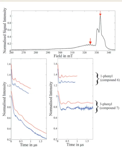
Fig. 5 Top: Field-sweep EPR spectrum depicting the DEER pump (dashed

red arrow) and detection (solid red arrow) positions used for the experiments on the 1-phenyl Cu(II)–NO_{and 3-phenyl Cu(}_II_)–NO_{systems (compounds}

6and7). Bottom: DEER traces (blue) with corresponding simulations (red) for molecules 1-phenyl Cu(II)–NO_(compound₆_{, upper traces) and 3-phenyl} Cu(II)–NO _(compound₇_{, lower traces). Left: Raw experimental data and} simulations. Right: Experimental form factors obtained after background correction and corresponding simulations. Simulations are based on the molecular conformations determined by DFT modelling to computef(t) and the relatedS(t), as defined by eqn (D) of the ESI,†beforecandkof eqn (2) and eqn (B) of the ESI†are optimized to fit the traces.

[image:7.595.308.548.314.602.2] [image:7.595.49.287.519.674.2]

(8)

stringent conditions, lead to a large variation in the obtained anglesw,gandZdefining the orientation.

No X-ray structures of the model molecules1–8 were avail-able, however their chemical structures are known and this allowed distributions of molecular geometries to be built using DFT as described in the Methods section. Each molecular geometry determined by DFT defines the relative orientations of the two paramagnetic centres and the correspondingg-matrices and copper hyperfine interactions needed as input for the orientation-selective DEER trace simulation.10 Summing the simulated traces over the set of molecular orientations provides the DEER simulation of the DFT conformation distribution. To test the accuracy of this approach, we compared the DEER experimental data with simulations computed using DFT derived models for the NO–NO, NO–Cu(II) and Cu(II)–Cu(II)

systems. The conformation distributions for each molecule are depicted in Fig. S3 (ESI†). For the NO–NOsystem good agreement was found between the distance distributions computed from the experimental data using DeerAnalysis4 _{and those obtained}

using the DFT model. Data for the NO_–NO_{system is provided} in the ESI†(Fig. S9).

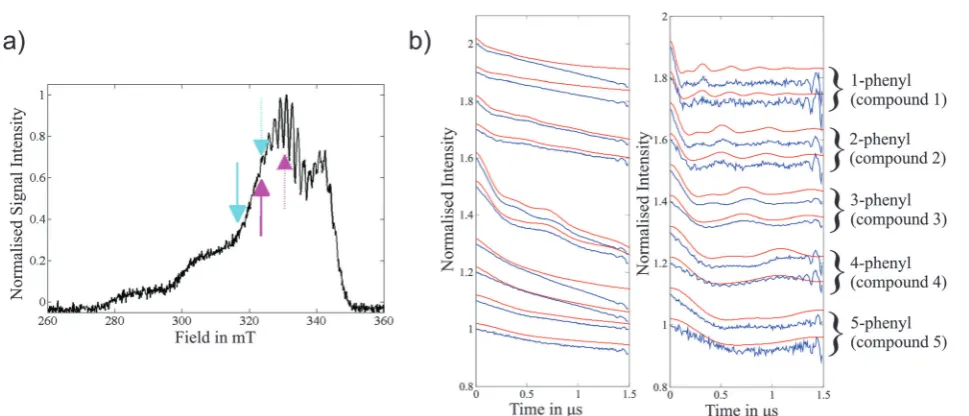
Fig. 5 and 6 show the DEER data and corresponding simula-tions for the NO_–Cu(_II_{) and the Cu(}_II_)–Cu(_II_{) model systems,} respectively. The excellent prediction of the simulated DEER traces as compared to the experimental traces for all systems demonstrates the accuracy of our DFT approach in modelling the set of molecular conformations.

As can be seen in Fig. 6b, there is significant variation in the modulation depths,D, of the traces recorded on the diﬀerent Cu(II)–Cu(II) molecules, and thus the modulation depth scaling

factors,c, were different (see eqn (2)). Thecvalue was, however,

consistent within all measurements taken for each sample since they used the same experimental tuning conditions and detection/pump frequency difference of Dn = 200 MHz, with only theB0field position changed. The variation in modulation

depths is due to slightly different labelling efficiencies of the systems and different pump pulse inversion efficiencies.6

DEER simulations with approximate conformation modelling

As shown above, the first principles DEER simulations computed from conformers with a defined molecular structure provide an accurate description of the experimental data. However, produ-cing the structural conformers is a complex task and knowledge of the chemical structure is required. As typically DEER is used to determine structure, we therefore now explore the utility of parameterised structural models that are generated from a mini-mum of structural information.

A number of models of varying sophistication have been described in the literature for systems including one or more Cu(II) centres.26,30,31Here we discuss six models (Fig. 7 upper

part), some of which are based upon the diﬀerent types of models trialled in the literature, and the corresponding DEER simulations (Fig. 7 lower part) for the case of the 3-phenyl Cu(II)–Cu(II) molecule (compound3). A seventh model (Fig. 8) is

also employed to investigate the limits of angular flexibility for the 3-phenyl Cu(II)–Cu(II) system.

Model 1 – DFT derived model (red).This is the DFT-based model described in detail above, for which simulated data agree well with experiment.

Model 2 – set of conformers with all angles allowed around rigid rods (green).Model 2 uses the same rigid rods (Fig. 1) as for model 1. However, rather than using the DFT calculations

Fig. 6 (a) Field-sweep EPR spectrum depicting experimental DEER pump (dashed arrows) and detection (solid arrows) positions for all five Cu(II)–Cu(II)

compounds. The cyan arrows correspond to the lower DEER traces (observer field 316.5 mT) and the magenta arrows the upper DEER traces (observer field 323.5 mT) for each compound in (b). (b) Experimental data for the 1- to 5-phenyl Cu(II)–Cu(II) compounds (molecules1–5) (blue) with corresponding simulations (red) that are based on the molecular conformers determined by DFT modelling. Labels on the right refer to both (b) plots. Left: Raw experimental DEER data. Right: Experimental form factorsf(t) after background removal. The experimentalf(t) amplitudes have been scaled usingcto match the simulated modulation depth. The high frequency oscillations at the end of the traces are nuclear modulation artefacts due to overlap of the pump and probe pulse excitation bandwidths.61

[image:8.595.60.545.432.640.2]

(9)

of the structural fragments to determine the energy and thus allowed rotations about the rods, all angles were allowed for all three rods. The simulated data is very similar to those of model 1. This is a result of the symmetry (axialg-matrix) and high angular flexibility of the Cu(II)–Cu(II) 3-phenyl system (compound3); in

model 1 rotations about the three rods cover almost 3601.

Model 3 – cone and linker bending angles model (yellow). This model was generated using similar parameters to those

employed by Bodeet al.:26,27_{free rotation was allowed around}

the axis of the linker within a cone of 221, which allows for flexibility around the amide linker and nitroxide moiety. The flexibility of the central linker was modelled in two halves around a central pivot point with each half being allowed a bending angle of 201. The model is detailed in Fig. S10 (ESI†). The distribution produced by this model is very similar to one of the two distributions determined in the DFT based model 1

Fig. 7 Top: Schematic representation of the six models trialled for the 3-phenyl Cu(II)–Cu(II) system (compound3), the axes correspond tox,yandzin Å,

the radius of the sphere in each case is 33.5 Å, the average inter-spin separation. The surrounding box colour corresponds to the simulated DEER traces in the lower part of the figure. All models havegzperpendicular to the plane formed by the four nitrogens. Thegzaxis of the detection centre is highlighted by a red line and the pump centre by a green line. Bottom: Simulated and experimental form factorsf(t) (i.e.background corrected experimental data). Left and right panels correspond to the DEER measurement positions cyan (observer field 316.5 mT) and magenta (observer field 323.5 mT), respectively, shown in Fig. 6a.

[image:9.595.61.533.47.528.2]

(10)

as shown in Fig. 7. As a consequence of the plane of symmetry of the Cu(II) porphyrin and the axial symmetry of the Cu(II)

g-matrix with thegzaxis perpendicular to this plane, the DEER traces generated by this model are very similar to those calculated for model 1, despite the absence of the second cluster of orientations contributing in model 1. It should be noted that the second population cluster in model 1 is a result of the

planar symmetry of the porphyrin and the 1801 _periodic symmetry of the allowed conformations of the linker bonds (particularly the bonds either side of the amide moiety, notated A and B in Fig. S2, ESI†).

Model 4 – average structure computed from the DFT derived conformers (purple).Taking the average of all molecular orienta-tions in model 1, a single average molecular orientation was computed. However, whereas the DFT generated orientations had the gz axes approximately perpendicular to the vector between the two centres, when an average molecular structure is computedgzlies approximately parallel to the vector linking the two centres. Consequently this model generates markedly different simulated DEER traces which do not match the experi-ment. This ill-fitting model shows that a distribution of molecular positions and orientations cannot always be accurately described by a single average conformation.

Model 5 – single distance with isotropicg-tensor orientation (cyan).Keeping the distance between the two centres fixed, the relative orientation between the twog-matrices was allowed to vary without restriction. When the distribution is viewed in the g-tensor frame of one of the centres this yields a random spherical spatial distribution of the second centre with respect to the first, and a random orientation of theg-tensor of the second centre with respect to the first. This model corresponds to an isotropic angular distribution of the Cu(II) centres and

thus yields a DEER trace without any angular information. It is clear from a comparison with the simulated trace that there must be angular information encoded in the experimental data as this model does not adequately reproduce the features of the experimental traces.

Model 6 – distance distribution described by two separated spheres with limited gzorientations (black).This approach uses a model based upon the model coordinate system (definition of angles) described by Yanget al.30,31_{In this model each centre is}

evenly distributed within a sphere (ball) of adjustable radius. The position of the sphere (of radiusDR) for centre 2 is moved relative to centre 1 by rotating through an anglew swaway from thegzaxis of centre 1 which is fixed. In the peptide based model systems studied by Yanget al.the best fit between the model and the experimental data used a sphere radius (DR)Z 10% of the mean inter-spin distance,R, withswvalues ranging from 9–121_.

Here our model uses two spherical distributions of Cu(II)

centres, each sphere has a radius ofDR= 0.5 nm and is centred at the weighted average (x,y,z) coordinate derived from model 1, giving a mean inter-spin distance,R= 3.32 nm. In our model the radius of the spheres DR was chosen so that it would encompass both the maximum and minimum distances and relative spatial positions (angle) found in the DFT derived model 1. The centre of the second sphere was positioned at an anglew= 871, corresponding to the centre of one of the distribu-tions in model 1. In our model sw = 01 as the variation in w observed in model 1 is included within the radius of the spheres. Theg-tensors of the second centre with respect to the first have the same range of orientations as those determined from the DFT conformers of model 1 (further details are given in Fig. S11, ESI†).

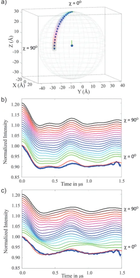
Fig. 8 Simulation for the 3-phenyl Cu(II)–Cu(II) molecule (compound3)

using model 7 that is parameterised by polar angle w and a uniform distribution ofgzvectors perpendicular to the spin–spin vector. (a) Shows thewrange (01to 901in 51intervals). (b) and (c) show the corresponding simulated DEER traces. Data collected at the magenta pulse positions (observer field 323.5 mT) in Fig. 6a is shown in (b) and data from the cyan pulse positions (observer field 316.5 mT) in Fig. 6a is plotted in (c). The colour code is consistent between the panels and the experimental data is shown as a thick blue line and is overlaid by the best fit wherew= 751.

[image:10.595.52.283.52.510.2]

(11)

The large degree of positional freedom provided in this model is seen to ‘wash out’ much of the structure in the DEER trace.

It is clear that a model using two spheres of fixed position and relatively large radius is a poor choice for these rod-like systems where the distance between the centres is well defined. In the model used by Yanget al.when studying copper centres attached to polypeptide chains, it is likely that a more even flexibility of the relative copper positions in all directions in their systems required the use of a relative large radius with respect to the inter-sphere separation in their ball-like model. It should also be noted that in their model a variation inwwas also included.30,31However, for both their systems and the rod like model systems studied here, it is not possible to completely describe the conformer distribution with a spherical distribu-tion for each centre.

Model 7 – position distribution around polar anglevwith gz

orientation around the spin–spin vector for fixed distance. Analysis of the Cu(II)–Cu(II) 3-phenyl (compound3) establishes that the orientation of thegzaxis of both centres is approximately perpendicular to the inter-spin vector. Model 7 thus employs this restriction and is parametrised by an azimuthal anglew(Fig. 4) and a fixed distance. The gz axis of centre 2 takes on all orientations perpendicular to the spin–spin vector. To compute a trace for any angle w, gz of centre 2 was rotated through 3601_{degrees about the inter-spin vector in 20}1_{steps and the} resulting 18 simulated DEER traces were summed.

Fig. 8 presents results for this model in one quadrant (w= 01 to 901_{) which is suﬃcient due to the axial symmetry of the} g-tensor (four-fold symmetry). These data show good agree-ment between the simulated and experiagree-mental DEER traces in the rangew= 65–901_{, establishing a structural restriction on} the distribution of the two centres. This result is consistent with the DFT derived model 1 and the conical geometric model 4 where similar limitations on the angular distribu-tions are found.

Computation of a distance distribution

Computation and validation of models to determine the orienta-tion and spatial distribuorienta-tion of two centres can be complicated and, as shown above, several diﬀerent models can adequately describe the experiment. In many cases the most important single piece of information is the inter-spin distance. Here we examine methods to extract this information independently of the relative orientation of the two centres.

The most commonly used method for extracting distance distribution information from DEER traces is Tikhonov regu-larization using kernel functions appropriate for nitroxide spin centres. These kernel functions depend only upon the inter-spin distance (defining a complete dipolar Pake pattern) and use an average nitroxide g-value (2.0023 in the DeerAnalysis software used here)56to compute the dipolar frequencies (odd):

odd¼ m_B2m₀

4ph gAgB

rAB3

13 cos2yAB

(4)

Here,gA=gBfor the pump and detection spins and the other

constants have their usual meanings.

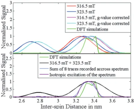
Initial processing of the two experimental traces for the 3-phenyl Cu(II)–Cu(II) model system (compound 3) using DeerAnalysis yielded distance distributions (red and blue traces, top panel Fig. 9) with an average distance for the main peak which deviated from the DFT model byca.0.1 nm (green trace, top panel Fig. 9). However, if the experimental distance distributions are corrected with the average Cu(II)–Cu(II)

3-phenyl (compound3)g-values excited by the pump and detec-tion pulses (magenta and cyan traces, top panel Fig. 9), then the agreement of the experimental and DFT distance distributions improves significantly. Theg-value correction used is (g= 2.0023 is used for nitroxides in DEER analysis):

rCuCu¼r2:0023

geff;pumpgeff;det 2:00232

1

3

(5)

Although the main peaks of both experimental g-value cor-rected distance distributions agree well with the DFT result, the trace collected at 323.5 mT also shows as significant peak around 2.75 nm. This peak is an artefact which is due to the orientation selection where high frequencies aroundn_J(y= 0, pin eqn (4)) are overrepresented in the DEER trace in compar-ison to a complete Pake pattern.

Within the restrictions of the deviations which occur due to diﬀering g-values the main peak of the distance distribution

Fig. 9 Distance distributions for the 3-phenyl Cu(II)–Cu(II) molecule

(compound3) computed from Tikhonov regularization as implemented in DeerAnalysis. Top: Distance distributions before and after Cu(II)g-values correction, for data recorded at 316.5 mT, redvs.magenta, and 323.5 mT, bluevs.cyan, respectively. At 316.5 mT;geff,pump= 2.1162 andgeff,det= 2.0981, at 323.5 mT;geff,pump= 2.0949 andgeff,det= 2.0668. For reference the distance distribution calculated from the DFT derived structural model is plotted in green (in both top and bottom panels). Bottom: Theg-value corrected distance distributions from a simulated trace computed with isotropic excitation and from an average trace which is the sum of 8 traces simulated for detection and pump pulses withDn = 100 MHz at fields evenly positioned across the Cu(II) spectrum. For comparison the distance distribution resulting from the sum of the traces recoded experimentally at 316.5 mT and 323.5 mT is also shown. All simulated traces use the DFT derived model as input and consequently are an average of 1000 structures.

[image:11.595.312.543.49.236.2]

(12)

can be obtained via Tikhonov regularization from measure-ments obtained around the gx/gy value positions since both

detection and pump pulses excite the gx/gy plane of orienta-tions,10_{leading to a strong representation of frequencies around}

n>(y=p/2, 3p/2 in eqn (4)), which is independent of the relative

spin centre orientations. This dominant representation of the n>turning point enables an approximate estimate of the mean

sample distance. To remove orientation effects it is necessary to excite all orientations of the centres with respect to one another. Theoretically this could be achieved using isotropic excitation of the whole spectrum (trace shown in the bottom panel of Fig. 9). It has been shown experimentally for bisnitroxide molecules that orientation effects in DEER traces can be strongly sup-pressed by averaging multiple DEER traces recorded at different fields with a constant frequency offset.57,58 A more accurate approach is to additionally vary the pump–probe offset,59 but this requires retuning the pulses between experiments which is not easy to automate. One thing that limits the accuracy of a summed trace approach is dealing with the distribution of orientations and correspondingg-values contributing to each trace which is difficult to include precisely in the analysis.59

Although these trace summing approaches require the measure-ment of a number of experimeasure-mental data sets, they simplify the analysis considerably by allowing a reliable mean distance and an estimate of the distance distribution to be extracted, typically viaTikhonov regularization, using for example DeerAnalysis.4A similar approach can be applied to copper centres and is trialled here for the 3-phenyl Cu(II)–Cu(II) model system (compound3).

DEER data was simulated using a constant offset ofDn= 100 MHz, and the field was shifted by steps of 10 mT (8 steps in total) so as to sample the whole Cu(II) field-sweep EPR spectrum. The

simulated DEER traces were summed and ag-value corrected distance distribution computed using DeerAnalysis and eqn (5) (trace shown in the bottom panel of Fig. 9).

Note that this method does not simultaneously sample all relative g-matrix orientations of the Cu(II) pairs. For example

with the detection pulses positioned atgz(which corresponds

to the lowest field position in the EPR spectrum) and a pulse oﬀset ofDn= 100 MHz between the detection and pump pulses, it is not possible to excite thegxandgypositions (ca.400 MHz

oﬀ-resonance fromgz). Nevertheless, both the distance

distribu-tion from the theoretical isotropic excitadistribu-tion and from the sum of the traces simulated across the Cu(II) spectrum agree well with

the DFT distribution (Fig. 9, bottom panel). In addition, the agreement of the distance distributions for the 8 summed traces and the theoretical simulation for full isotropic excitation is very good and therefore we can conclude that by measuring several traces across the Cu(II) spectrum we can adequately suppress orientation selection eﬀects in the summed trace.

As a comparison the distance distribution from the sum of the two experimental traces (trace shown in the bottom panel of Fig. 9) still has a strong contribution from the peak centred at 2.75 nm. Therefore, in this case summing two single traces, one of which primarily samplesgx/gyvalues (323.5 mT trace) and the

other of which includes a stronggzvalue component (316.5 mT

trace) is not suﬃcient to satisfactorily suppress orientation

selection eﬀects. The time traces for the simulated theoretical isotropic excitation and the 8 summed DEER traces collected across the copper spectrum with constant pump–probe frequency offset are shown in Fig. S13 (ESI†).

Conclusions

To examine the utility of orientation-selective DEER spectro-scopy as applied to systems containing Cu(II) centres we chose a

protein homo-dimer with a single relative orientation between two Cu(II) centres. Furthermore, a set of model compounds with

diﬀerent distances between the two Cu(II) centres that exhibit a

range of conformers in frozen solution has been investigated. X-band orientation-selective DEER on the rigidly held Cu(II)

centres of a homodimer of AGAO provided an accurate distance distribution measurement. However, in this case of a single molecular orientation the DEER data provided only a broad range of possible orientations all of which satisfactorily described the experimental DEER data. This uncertainty in the orientation of the two copper centres is due to the intrinsic limitations resulting from the spin Hamiltonian symmetry, and also the uncertainty in orientating theg-matrix, which is required to compute the DEER orientation selectivity. However, the orientation-selective DEER data can still be exploited to limit the relative orientations of the two paramagnetic centres to a reasonably small range. In cases where theg-tensor orientation is not known it could be deter-mined experimentally through a detailed analysis of orientation-selective ENDOR and/or HYSCORE data in conjunction with the structure of the paramagnetic centre if it is known.60

A series of model systems; NO–NO, NO–Cu(II) and Cu(II)–

Cu(II) (1–8), were employed to determine how accurately the conformation ensemble could be defined from the DEER data alone. Firstly the conformers for each model molecule (1–8) in frozen-solution were accurately determined using DFT calcula-tions employing a fragment approach. These computed confor-mer distributions yielded DEER simulations for the NO_–Cu(_II₎ and Cu(II)–Cu(II) systems that provided an excellent description

of the experiments with all detailed oscillation features in the DEER traces being accurately modelled.

A satisfactory mean distance and distance distribution esti-mate with orientation artefacts strongly suppressed can be obtained from a Tikhonov regularization analysis from mea-surements on Cu(II) centres by summing a set of traces that

select diﬀerent orientations and using eﬀective Cu(II)g-values

(geﬀ,pumpandgeﬀ,det).

Moreover, various models were employed to ascertain the structural information, in particular orientation information, derivable from the DEER traces themselves. The utility and reliability of these various models was compared to the DFT computed conformer distribution. This analysis was carried out on the Cu(II)–Cu(II) compound3.

As revealed by DFT computations (model 1) compound3has a conformation distribution with a relatively narrow distance distribution but a complicated conformation distribution that defines two separate populations (Fig. 7). The gzaxis of the

(13)

g-matrix is approximately perpendicular to the axis joining the two Cu(II) centres but approximately randomly orientated around this axis.

The structural models 2, 3 and 7 provided satisfactory simulations of the DEER data. Model 2 represents a full set of conformers based on the known structure but, unlike model 1, without any population cut-oﬀ. This model maintained both a suitable distance distribution to describe the DEER data and the gz axis approximately perpendicular to the Cu–Cu axis. Model 3 employs structural parameters (angles and distances) which approximate well the DFT derived conformer distribu-tion; the linker length and amount of bend provide useful para-meters to define the distance distribution between the Cu(II)

centres. Furthermore, in model 3 thegzaxis is also maintained approximately perpendicular to the linker axis and randomly orientated around it. This model thus provides DEER simula-tions that match well the experimental data. Model 7 essentially is a statement of the orientation information that can be uniquely extracted from the DEER data: the gz axis is fixed perpendicular to the Cu–Cu axis, although allowed to freely rotate about this axis, and the polar anglewbetween the Cu(II)

centres was varied. It was found thatw= 751provided the best fit to the experimental data.

Models using a single average structure (model 4) or a single distance and random g-matrix orientation (model 5) failed. Likewise models with a large distance distribution (model 6) failed, even if thegzaxis orientation was restricted.

This analysis of various models demonstrates that useful structural information can be extracted from orientation-selective DEER. Distance information can be determined and restrictions can be placed on the possible relative orientations of the two Cu(II) paramagnetic centres that can be used to support/constrain structural models. Particularly in cases where there is very limited structural information available to guide the DEER trace analysis, we recommend firstly to obtain an estimate of the distance distribution from a summed trace approach to strongly suppress orientation artefacts, then building the struc-tural model to simulate the orientation-selective DEER traces constrained by this distance distribution.

Acknowledgements

We gratefully acknowledge financial support from the EPSRC, BBSRC and Royal Society. JRH thanks the ARC (FT120100421) for financial support. JEL and AMB would like to thank Uni-versity College, Oxford for financial support. JEL would also like to thank The Royal Society for a University Research Fellowship. TGG and AMB were supported by a BBSRC studentships. We are grateful to the Department of Chemistry’s Research Services (University of Oxford) for their support and advice (Mass Spectrometry, NMR, CAESR and X-ray Crystallography). We thank Prof. David Dooley (Rhode Island) for providing an Arthrobacter globiformisamine oxide clone and Prof. Thomas Prisner (Goethe University Frankfurt) for useful discussions. Molecular graphics images were produced using the UCSF

Chimera package from the Resource for Biocomputing, Visua-lization, and Informatics at the University of California, San Francisco (supported by NIH P41 RR-01081). We acknowledge the Oxford Supercomputing Centre for the computing power used for the ADF calculations.

Notes and references

1 M. Pannier, S. Veit, A. Godt, G. Jeschke and H. W. Spiess, J. Magn. Reson., 2000,142, 331–340.

2 R. Ward, A. Bowman, E. Sozudogru, H. El-Mkami, T. Owen-Hughes and D. G. Norman, J. Magn. Reson., 2010, 207, 164–167.

3 A. P. Todd, J. Cong, F. Levinthal, C. Levinthal and W. L. Hubbell,Proteins, 1989,6, 294–305.

4 G. Jeschke, V. Chechik, P. Ionita, A. Godt, H. Zimmermann, J. Banham, C. R. Timmel, D. Hilger and H. Jung,Appl. Magn. Reson., 2006,30, 473–498.

5 A. M. Bowen, C. E. Tait, C. R. Timmel and J. R. Harmer, in Structure and bonding: spin-labels and intrinsic paramagnetic centres in the biosciences: structural information from distance measurements, ed. C. R. Timmel and J. R. Harmer, Spring-erLink, 2013, vol. 152.

6 D. Margraf, B. E. Bode, A. Marko, O. Schiemann and T. F. Prisner,Mol. Phys., 2007,105, 2153–2160.

7 Y. Polyhach, E. Bordignon, R. Tschaggelar, S. Gandra, A. Godt and G. Jeschke,Phys. Chem. Chem. Phys., 2012,14, 10762–10773.

8 R. G. Larsen and D. J. Singel, J. Chem. Phys., 1993, 98, 5134–5146.

9 S. Milikisyants, E. J. J. Groenen and M. Huber, J. Magn. Reson., 2008,192, 275–279.

10 J. E. Lovett, A. M. Bowen, C. R. Timmel, M. W. Jones, J. R. Dilworth, D. Caprotti, S. G. Bell, L. L. Wong and J. Harmer,Phys. Chem. Chem. Phys., 2009,11, 6840–6848. 11 I. M. C. van Amsterdam, M. Ubbink, G. W. Canters and

M. Huber,Angew. Chem., Int. Ed., 2003,42, 62–64.

12 M. Ubbink, J. A. R. Worrall, G. W. Canters, E. J. J. Groenen and M. Huber,Annu. Rev. Biophys. Biomol. Struct., 2002,31, 393–422.

13 X. Zheng, L. Wu, D. Gao, N. Chi, Q. Lin and J. Hu, Spectro-chim. Acta, Part A, 2003,59, 1751–1755.

14 C. J. Sarell, C. D. Syme, S. E. J. Rigby and J. H. Viles, Biochemistry, 2009,48, 4388–4402.

15 S. Atwell, E. Meggers, G. Spraggon and P. G. Schultz,J. Am. Chem. Soc., 2001,123, 12364–12367.

16 E. Meggers, P. L. Holland, W. B. Tolman, F. E. Romesberg and P. G. Schultz,J. Am. Chem. Soc., 2000,122, 10714–10715. 17 M. K. Schlegel, L. Essen and E. Meggers,J. Am. Chem. Soc.,

2008,130, 8158–8159.

18 N. Zimmermann, E. Meggers and P. G. Schultz, Bioorg. Chem., 2004,32, 13–25.

19 Z. Yang, G. Jime´nez-Ose´s, C. J. Lo´pez, M. D. Bridges, K. N. Houk and W. L. Hubbell, J. Am. Chem. Soc., 2014, 136, 15356–15365.

(14)

20 Z. Yang, M. R. Kurpiewski, M. Ji, J. E. Townsend, P. Mehta, L. Jen-Jacobson and S. Saxena,Proc. Natl. Acad. Sci. U. S. A., 2012,109, E993–E1000.

21 T. F. Cunningham, M. R. Putterman, A. Desai, W. S. Horne and S. Saxena,Angew. Chem., Int. Ed., 2015,54, 6330–6334. 22 T. F. Cunningham, M. D. Shannon, M. R. Putterman, R. J. Arachchige, I. Sengupta, M. Gao, C. P. Jaroniec and S. Saxena,J. Phys. Chem. B, 2015,119, 2839–2843.

23 J. H. van Wonderen, D. N. Kostrz, C. Dennison and F. MacMillan,Angew. Chem., Int. Ed., 2013,52, 1990–1993. 24 G. E. Merz, P. P. Borbat, A. J. Pratt, E. D. Getzoﬀ, J. H. Freed

and B. R. Crane,Biophys. J., 2014,107, 1669–1674.

25 E. Narr, A. Godt and G. Jeschke,Angew. Chem., Int. Ed., 2002, 41, 3907–3910.

26 B. E. Bode, J. Plackmeyer, M. Bolte, T. F. Prisner and O. Schiemann,J. Organomet. Chem., 2009,694, 1172–1179. 27 B. E. Bode, J. Plackmeyer, T. F. Prisner and O. Schiemann,

J. Phys. Chem. A, 2008,112, 5064–5073.

28 D. Abdullin, N. Florin, G. Hagelueken and O. Schiemann, Angew. Chem., Int. Ed., 2015,54, 1827–1831.

29 Z. Yang, J. Becker and S. Saxena,J. Magn. Reson., 2007,188, 337–343.

30 Z. Yang, D. Kise and S. Saxena,J. Phys. Chem. B, 2010,114, 6165–6174.

31 Z. Yang, M. Ji and S. Saxena,Appl. Magn. Reson., 2010,39, 487–500.

32 J. S. Becker and S. Saxena, Chem. Phys. Lett., 2005, 414, 248–252.

33 E. Aronoﬀ-Spencer, C. S. Burns, N. I. Avdievich, G. J. Gerfen, J. Peisach, W. E. Antholine, H. L. Ball, F. E. Cohen, S. B. Prusiner and G. L. Millhauser,Biochemistry, 2000,39, 13760–13771.

34 C. S. Burns, E. Aronoﬀ-Spencer, G. Legname, S. B. Prusiner, W. E. Antholine, G. J. Gerfen, J. Peisach and G. L. Millhauser, Biochemistry, 2003,42, 6794–6803.

35 G. L. Millhauser,Acc. Chem. Res., 2004,37, 79–85.

36 A. Marko, D. Margraf, P. Cekan, S. T. Sigurdsson, O. Schiemann and T. F. Prisner,Phys. Rev. E: Stat., Non-linear, Soft Matter Phys., 2010,81, 1–9.

37 A. Marko and T. F. Prisner,Phys. Chem. Chem. Phys., 2013, 15, 619–627.

38 R. Luguya, L. Jaquinod, F. R. Fronczek, A. G. H. Vicente and K. M. Smith,Tetrahedron, 2004,60, 2757–2763.

39 A. D. Adler, F. R. Longo, J. D. Finarell, J. Goldmach, J. Assour and L. Korsakof,J. Org. Chem., 1967,32, 476.

40 A. Godt, C. Franzen, S. Veit, V. Enkelmann, M. Pannier and G. Jeschke,J. Org. Chem., 2000,65, 7575–7582.

41 G. A. Juda, J. A. Bollinger and D. M. Dooley,Protein Expres-sion Purif., 2001,22, 455–461.

42 R. E. Martin, M. Pannier, F. Diederich, V. Gramlich, M. Hubrich and H. W. Spiess, Angew. Chem., Int. Ed., 1998,37, 2834–2837.

43 A. D. Milov, K. M. Salikhov and M. D. Shchirov,Sov. Phys., Solid State, 1981,23, 565–569.

44 A. D. Milov, A. B. Ponomarev and Y. D. Tsvetkov,Chem. Phys. Lett., 1984,110, 67–72.

45 J. E. Lovett, B. W. Lovett and J. Harmer,J. Magn. Reson., 2012,223, 98–106.

46 G. Jeschke, inStructure and bonding: spin-labels and intrinsic paramagnetic centres in the biosciences: structural information from distance measurements, ed. C. R. Timmel and J. Harmer, SpringerLink, 2012, vol. 152.

47 SCM, http://www.scm.com/.

48 G. te Velde, F. M. Bickelhaupt, E. J. Baerends, C. Fonseca Guerra, S. J. A. van Gisbergen, J. G. Snijders and T. Ziegler, J. Comput. Chem., 2001,22, 931–967.

49 F. Neese,Magn. Reson. Chem., 2004,42, S187–S198. 50 R. Prabhakar, P. E. M. Siegbahn, B. F. Minaev and H. Ågren,

J. Phys. Chem. B, 2004,108, 13882–13892.

51 Y. Pontillon, A. Grand, T. Ishida, E. Lelie`vre-Berna, T. Nogami, E. Ressouche and J. Schweizer,J. Mater. Chem., 2000,10, 1539–1546.

52 S. Kishishita, T. Okajima, M. Kim, H. Yamaguchi, S. Hirota, S. Suzuki, S. Kuroda, K. Tanizawa and M. Mure,J. Am. Chem. Soc., 2003,125, 1041–1055.

53 T. G. Brown and B. M. Hoﬀman,Mol. Phys., 2006,39, 1073–1109. 54 M. Kim, T. Okajima, S. Kishishita, M. Yoshimura, A. Kawamori, K. Tanizawa and H. Yamaguchi,Nat. Struct. Biol., 2002,9, 591–596.

55 S. Ghosh, J. Cirera, M. A. Vance, T. Ono, K. Fujisawa and E. I. Solomon,J. Struct. Biol., 2008,130, 16262–16273. 56 G. Jeschke, 2012, http://www.epr.ethz.ch/software/index. 57 A. Godt, M. Schulte, H. Zimmermann and G. Jeschke,

Angew. Chem., Int. Ed., 2006,45, 7560–7564.

58 G. Jeschke, M. Sajid, M. Schulte, N. Ramezanian, A. Volkov, H. Zimmermann and A. Godt,J. Am. Chem. Soc., 2010,132, 10107–10117.

59 A. Marko, V. Denysenkov, D. Margraf, P. Cekan, O. Schiemann, S. T. Sigurdsson and T. F. Prisner,J. Am. Chem. Soc., 2011,133, 13375–13379.

60 J. A. B. Abdalla, A. M. Bowen, S. G. Bell, L. L. Wong, C. R. Timmel and J. Harmer, Phys. Chem. Chem. Phys., 2012,14, 6526–6537.

61 G. Jeschke,Annu. Rev. Phys. Chem., 2012,63, 419–446.