C
2014. The American Astronomical Society. All rights reserved. Printed in the U.S.A.
THE GALAXY CLUSTER MID-INFRARED LUMINOSITY FUNCTION AT 1
.
3
< z <
3
.
2
Dominika Wylezalek1, Jo¨el Vernet1, Carlos De Breuck1, Daniel Stern2, Mark Brodwin3, Audrey Galametz4,
Anthony H. Gonzalez5, Matt Jarvis6,7, Nina Hatch8, Nick Seymour9, and Spencer A. Stanford10,11
1European Southern Observatory, Karl-Schwarzschildstr.2, D-85748 Garching bei M¨unchen, Germany 2Jet Propulsion Laboratory, California Institute of Technology, 4800 Oak Grove Drive, Pasadena, CA 91109, USA 3Department of Physics and Astronomy, University of Missouri, 5110 Rockhill Road, Kansas City, MO 64110, USA
4INAF-Osservatorio di Roma, Via Frascati 33, I-00040, Monteporzio, Italy 5Department of Astronomy, University of Florida, Gainesville, FL 32611, USA
6Astrophysics, Department of Physics, Keble Road, Oxford OX1 3RH, UK 7Physics Department, University of the Western Cape, Bellville 7535, South Africa
8School of Physics and Astronomy, University of Nottingham, University Park, Nottingham, NG7 2RD, UK 9CASS, P.O. Box 76, Epping, NSW, 1710, Australia
10Physics Department, University of California, Davis, CA 95616, USA
11Institute of Geophysics and Planetary Physics, Lawrence Livermore National Laboratory, Livermore, CA 94550, USA
Received 2013 November 6; accepted 2014 March 7; published 2014 April 10
ABSTRACT
We present 4.5μm luminosity functions for galaxies identified in 178 candidate galaxy clusters at 1.3< z <3.2.
The clusters were identified asSpitzer/Infrared Array Camera (IRAC) color-selected overdensities in the Clusters
Around Radio-Loud AGN project, which imaged 420 powerful radio-loud active galactic nuclei (RLAGNs) at
z > 1.3. The luminosity functions are derived for different redshift and richness bins, and the IRAC imaging
reaches depths of m∗+ 2, allowing us to measure the faint end slopes of the luminosity functions. We find that
α = −1 describes the luminosity function very well in all redshift bins and does not evolve significantly. This
provides evidence that the rate at which the low mass galaxy population grows through star formation gets quenched and is replenished by in-falling field galaxies does not have a major net effect on the shape of the luminosity function.
Our measurements for m∗ are consistent with passive evolution models and high formation redshifts (zf ∼ 3).
We find a slight trend toward fainterm∗ for the richest clusters, implying that the most massive clusters in our
sample could contain older stellar populations, yet another example of cosmic downsizing. Modeling shows that a contribution of a star-forming population of up to 40% cannot be ruled out. This value, found from our targeted
survey, is significantly lower than the values found for slightly lower redshift, z ∼ 1, clusters found in
wide-field surveys. The results are consistent with cosmic downsizing, as the clusters studied here were all found in the vicinity of RLAGNs—which have proven to be preferentially located in massive dark matter halos in the richest environments at high redshift—and they may therefore be older and more evolved systems than the general protocluster population.
Key words: galaxies: active – galaxies: clusters: general – galaxies: evolution – galaxies: formation – galaxies: high-redshift – galaxies: luminosity function, mass function – techniques: photometric
Online-only material:color figures, machine-readable table
1. INTRODUCTION
Many attempts have been made to measure the formation epoch of galaxy clusters, generally finding high formation
redshifts,zf ∼2–4. Studies focusing on galaxy colors provide
insight into when stellar populations formed (e.g., Stanford et al.
1998; Holden et al. 2004; Eisenhardt et al. 2008), while the
assembly of galaxies and their evolution can be measured by analyzing the fundamental plane or galaxy luminosity functions
(e.g., van Dokkum & Stanford2003; Mancone et al.2010).
As a few examples, Eisenhardt et al. (2008) infer stellar
formation redshifts ofzf >4 for cluster galaxies by comparing
their I −[3.6] colors to passive galaxy evolution models.
Studying the color and the scatter of the main sequence,
Mei et al. (2006) infer a mean luminosity-weighted formation
redshift ofzf >2.8 for cluster ellipticals in two high-redshift
clusters in the Lynx supercluster. Earlier formation epochs are inferred for galaxies closer to the cores, with early-type galaxies
within 1 arcmin of the cluster centers havingzf > 3.7. Kurk
et al. (2009), who also look at the position of the red sequence
in color–magnitude diagrams and compare them to theoretical
predictions, inferzf ∼ 3 for a protocluster at z = 1.6. By
comparing the fundamental plane of a Lynx cluster atz=1.27
to the fundamental plane of the nearby Coma cluster, van
Dokkum & Stanford (2003) infer a stellar formation redshift
of zf = 2.6 for the distant cluster with passive evolution
thereafter.
Studying the mid-infrared (mid-IR) luminosity function at
high redshifts (1 < z < 3) probes rest-frame near-infrared
(near-IR) emission (J, H, K), which is a good proxy for stellar
mass for all but the youngest starbursting galaxies (Muzzin et al.
2008; Ilbert et al.2010). Such studies have shown that the bulk
of the stellar mass in clusters is already in place byz∼1.3 (e.g., Lin et al.2006; Muzzin et al.2008; Mancone et al.2010) and that
α, the faint end slope of the galaxy luminosity function, does not
evolve significantly with redshift (e.g., de Propris et al.1998;
Muzzin et al.2007; Strazzullo et al.2010; Mancone et al.2012).
It seems that processes that might lead to a substantial increase in mass, such as mergers and star formation, and processes that would strip mass away from the cluster, such as galaxy-galaxy interactions or galaxy harassment, either balance each other or do not to play an important role in cluster evolution.
On the other hand, there is evidence for considerable
16 spectroscopically confirmed galaxy clusters at 1< z <1.5 selected from the IRAC Shallow Cluster Survey (ISCS;
Eisen-hardt et al.2008), Brodwin et al. (2013) show that star
forma-tion is occurring at all radii and increases toward the core of the cluster for clusters atz >1.4. These clusters were identified as three-dimensional overdensities in the Bo¨otes Survey (Stanford
et al.2005; Elston et al.2006; Eisenhardt et al.2008) using a
photometric redshift probability distribution and wavelet
analy-sis (Brodwin et al.2006). Brodwin et al. (2013) observe a rapid
truncation of star formation betweenz ∼ 1.5 and z ∼ 1, by
which time the cores of the clusters become mostly quiescent. Investigating the color and scatter of the red sequence galaxies,
Snyder et al. (2012) conclude that atz ∼ 1.5 significant star
formation is occurring and that at this redshift the red sequence in the centers of clusters was rapidly growing.
In a related analysis also using the Bo¨otes cluster sample,
Mancone et al. (2010) measured the evolution of the mid-IR
luminosity function for a sample of galaxy clusters spanning
0.3 < z < 2. By measuring the luminosity function and
the evolution ofm∗ compared to theoretical passive evolution
models, Mancone et al. (2010) found zf ∼ 2.4 for the low
redshift (z < 1.3) portion of their cluster sample. At higher
redshift (1.3< z <1.8) a significant deviation from the passive models was measured which could most likely be explained by ongoing mass assembly at those redshifts. However, the highest redshift bins suffered from small sample sizes.
This paper aims to continue and complement these previous results and to extend the luminosity function analysis to higher redshift. We study the evolution of the luminosity function of almost 200 galaxy cluster candidates at 1.3 < z <3.2 discov-ered through the Clusters Around Radio Loud AGN (CARLA)
project (Wylezalek et al.2013). The clusters were found in the
fields of radio-loud active galactic nuclei (RLAGNs), includ-ing both typical unobscured (e.g., type-1) radio-loud quasars (RLQs) and obscured (e.g., type-2) RLAGN, also referred to as radio galaxies (RGs). Significant research stretching back many decades shows that RLAGN belong to the most massive galaxies
in the universe (Lilly & Longair1984; Rocca-Volmerange et al.
2004; Seymour et al.2007; Targett et al.2012) and are
prefer-entially located in rich environments up to the highest redshifts
(e.g., Minkowski 1960; Stern et al. 2003; Kurk et al. 2004;
Galametz et al.2012; Venemans et al.2007; Hutchings et al.
2009; Hatch et al.2011; Matsuda et al.2011; Mayo et al.2012;
Husband et al.2013; Ramos Almeida et al. 2013; Wylezalek
et al.2013). As described in Wylezalek et al. (2013), the
selec-tion of candidate cluster members in the vicinity of the CARLA targets is based purely on the mid-IR colors of galaxies around a luminous RLAGN with a spectroscopic redshift. The selection is thus independent of galaxy age, morphology, or the presence of a red sequence; we discuss the selection in more detail in
Section6. This sample allows us to perform a statistical study
of the mid-IR luminosity functions of a large sample of very high redshift galaxy clusters, achieving statistics never before achieved at these early epochs.
The paper is structured as follows: Section 2 describes
the observations and the cluster sample used in this work,
Section3describes the fitting procedure and estimation of the
uncertainties while the results are presented in Section 4. In
Section5, we explain the robustness tests carried out and discuss
our measurements in Section6. Section7summarizes the work.
Throughout the paper, we assumeH0 = 70 km s−1 Mpc−1,
Ωm=0.3,ΩΛ=0.7. All magnitudes and colors are expressed
in the AB photometric system unless stated otherwise.
2. DATA
2.1. Observations and Data Reduction
As part of theSpitzersnapshot program CARLA, we observed
the fields of 209 high-redshift radio galaxies (HzRGs) and 211 RLQs at 1.3< z <3.2. A description of the sample selection, observation strategy, data reduction, source extraction, determi-nation of completeness limits, and initial scientific results are
given in Wylezalek et al. (2013).
Briefly, the fields, covering 5.2 × 5.2 each, corresponding
to a physical size of ∼2.5×2.5 Mpc for the redshift range
of the targeted RLAGN, were mapped with the Infrared Array
Camera (IRAC; Fazio et al.2004) on board theSpitzer Space
Telescope at 3.6 and 4.5 μm (referred to as IRAC1 and IRAC2). The total exposure times give similar depths for both channels with the IRAC2 observations having been tailored to be slightly deeper for our intended science. The HzRG and RLQ samples have been matched with respect to their redshift and
radio-luminosity distributions. TheL500MHz–zplane is covered
relatively homogeneously in order to be able to study the environments around the AGN as a function of both redshift and radio luminosity.
The data were reduced using the MOPEX (Makovoz &
Khan 2005) package and source extraction was performed
using SExtractor (Bertin & Arnouts 1996) in dual image
mode with the IRAC2 image serving as the detection image. The CARLA completeness was measured by comparing the
CARLA number counts with number counts from theSpitzer
UKIDSS Ultra Deep Survey (SpUDS, PI: J. Dunlop) survey.
The SpUDS survey is a SpitzerCycle 4 legacy program that
observed∼1 deg2 in the UKIDDS UDS field with IRAC and
the Multiband Imaging Spectrometer (Rieke et al.2004) aboard
Spitzer. SpUDS reaches 5σ depths of ∼1 μJy (mag 24). We determine 95% completeness of CARLA at magnitudes of [3.6]=22.6 (=3.45μJy) and [4.5]=22.9 (=2.55μJy).
2.2. Cluster Sample
The cluster candidates studied in this paper were identified as IRAC color-selected galaxy overdensities in the fields of CARLA RLAGN. In order to isolate galaxy cluster candidates,
we first identify high-redshift sources (z > 1.3) by applying
the color cut [3.6]−[4.5] −0.1 (e.g., Papovich2008). This
color selection has proven to be very efficient at identifying high-redshift galaxies independent of their evolutionary stage.
A negativek-correction, caused by the 1.6μm bump that enters
the IRAC bands atz ∼1, leads to an almost constant IRAC2
apparent magnitude atz >1.3 and a red [3.6]−[4.5] color (Stern
et al.2005; Eisenhardt et al.2008; Wylezalek et al.2013). We
apply a counts-in-cells analysis to such color-selected IRAC sources, which we simply refer to as IRAC-selected sources, to identify overdense fields.
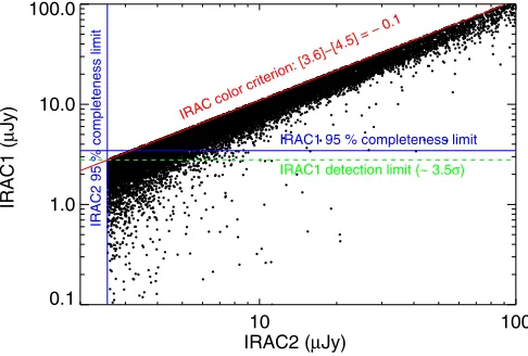
Specifically, we define a source to be an IRAC-selected source if (1) it is detected above the IRAC2 95% completeness limit
and above an IRAC1 flux of 2.8μJy (3.5σdetection limit) and
has a color of [3.6]−[4.5]> −0.1 or (2) it is detected above the IRAC2 95% completeness limit and has an IRAC1 flux <2.8μJy but has a color>−0.1 at the 3.5σ detection limit of
the IRAC1 observation (e.g., Figure1). This refined criterion
means that all IRAC-selected sources are 95% complete in
IRAC2 down to [4.5]=22.9 (=2.55μJy) but are not necessarily
Table 1
The CARLA Sample (in R.A. order)
Name R.A. Decl. z log(L500) Σ Type
(W Hz−1) (arcmin2)
USS0003−019 00:06:11.20 −01:41:50.2 1.54 27.86 11.2 HzRG
PKS_0011−023 00:14:25.50 −02:05:56.0 2.08 28.15 12.1 HzRG
MRC_0015−229 00:17:58.20 −22:38:03.80 2.01 28.32 17.9 HzRG
BRL0016−129 00:18:51.40 −12:42:34.6 1.59 29.02 17.2 HzRG
MG0018+0940 00:18:55.20 +09:40:06.9 1.59 28.39 14.7 HzRG
Notes.The surface densities for fields contaminated by, e.g., bright stars are denoted as “N.”
(This table is available in its entirety in a machine-readable form in the online journal. A portion is shown here for guidance regarding its form and content.)
10 100
IRAC2 (μJy) 0.1
1.0 10.0 100.0
IRAC1 (
μ
Jy)
IRAC2 95 % completeness limit
[image:3.612.47.290.215.379.2]IRAC1 detection limit (~ 3.5σ) IRAC1 95 % completeness limit IRAC color criterion: [3.6]−[4.5] = − 0.1
Figure 1.IRAC1 flux density vs. IRAC2 flux density for all sources in CARLA that pass the color criterion [3.6]−[4.5]> −0.1 (red line). The IRAC1 and IRAC2 95% completeness limits are shown by the blue horizontal and vertical lines, respectively. The IRAC1 detection limit used in the color criterion analysis (see Section2.2) is shown by the green dashed line. To build IRAC2 luminosity functions, a clear IRAC1 detection is not necessary, and we, therefore, focus on the IRAC2 luminosity function in this paper. The IRAC1 luminosity functions are presented in theAppendix.
(A color version of this figure is available in the online journal.)
We measure the density of IRAC-selected sources in a radius of 1 arcmin centered on the RLAGN and compare it to the mean blank-field density. A radius of 1 arcmin corresponds to
∼500 kpc over the targeted redshift range and matches typical
sizes forz >1.3 mid-IR selected clusters with log(M200/M)∼
14.2 (e.g., Brodwin et al.2011). The typical blank-field density
of IRAC-selected sources was measured by placing roughly 500 independent apertures of 1 arcmin radius onto the SpUDS field with its catalogs having been cut at the CARLA depth. Since the
publication of Wylezalek et al. (2013), 33 new CARLA fields
have been observed, and we provide the full table of CARLA fields and their overdensities in the online journal. A short,
example version is presented in Table1.
In Wylezalek et al. (2013), we used the IRAC1 95%
complete-ness limit of 3.45μJy as the IRAC1 limit in the color selection
process, rather than the 3.5σ detection limit of 2.8μJy used
above. As the IRAC1 95% completeness limit is brighter than the IRAC2 95% completeness limit, this IRAC1 limit together with the color criterion introduced an artificially brighter IRAC2
limit ([4.5]=22.7, 3.0μJy). In this work, we therefore raise the
IRAC1 limiting magnitude to [3.6]=22.8 (=2.8μJy), i.e., we
lower the flux density cut, to include all IRAC2 sources down to
the formal completeness limit of [4.5]=22.9. This new IRAC1
flux density cut still corresponds to a>3.5σ detection. This is
0 10 20 30
density (arcmin-2)
0 5 10 15 20
percentage of fields
CARLA SpUDS
> 2 σ
2.5 − 3.5 σ
> 3.5 σ
0 10 20 30
Figure 2.Histogram of the surface densities of IRAC-selected sources in the CARLA fields and the SpUDS survey. Surface densities are measured in circular regions of radiusr=1 arcmin. The Gaussian fit to the low-density half of the SpUDS density distribution is shown by the dashed black curve, giving ΣSpUDS =9.6±2.1 arcmin−2. The gray shaded area shows all SpUDS cells
with a surface density ofΣSpUDS=9.6±2.1 arcmin−2, which are used to derive
the blank field luminosity function. CARLA clusters are defined as fields with a surface density ofΣCARLA>2σ. In this paper, however, we also study the
dependence of the luminosity function on the CARLA overdensity and repeat the analysis for fields with 2.5σ < ΣCARLA < 3.5σ andΣCARLA > 3.5σ.
The fields that go into those analyses are shown by the pink shaded regions, as indicated.
(A color version of this figure is available in the online journal.)
necessary as we are aiming to include as many faint sources as possible in the analysis. We apply this refined color criterion to the CARLA and SpUDS fields and plot the distribution of their densities in Figure2.
Promising galaxy cluster fields are defined as fields that
are overdense by at least 2σ (ΣCARLA > ΣSpUDS+ 2σSpUDS;
Wylezalek et al. 2013). This criterion is met by 46% of the
CARLA fields: 27% are3σoverdense and 11% are overdense
[image:3.612.318.565.215.470.2]Note that this selection is a measure of the overdensity signal compared to a blank field, i.e., to a distribution of cell densities centered on random positions. Since the sample is selected using specific galaxies, RLAGN, there will always be at least one source in the overdensity. As all galaxies are clustered to some
extent (Coil2013), the exact measurement of the overdensity
signal of RLAGN would be to compare it to a distribution of background cells centered on random galaxies not random positions.
However, the average number density of IRAC-selected sources in SpUDS is very high, on average 34 sources per
aperture with radius r = 1 arcmin. This means that if the
IRAC-selected sources were extended and filled the aperture
maximally, their radius would only berext=10.3 arcsec and the
average distance between two sources would be 2×rext=20.6
arcsec. We repeated the blank-field analysis by measuring the densities in roughly 500 apertures centered on random SpUDS IRAC-selected sources. Because of the large aperture radius
of r = 1 arcmin and small rext, the difference between the
two background measurements is not significant (ΣSpUDS =
10.3±2.6 arcmin−2compared toΣSpUDS=9.6±2.1 arcmin−2,
see Section 3.2). Since we will work with the blank field
background for the luminosity function (LF) analysis and to
be consistent with Wylezalek et al. (2013), we show the SpUDS
blank field distribution in Figure2.
Wylezalek et al. (2013) shows that the radial density distribu-tion of the IRAC-selected sources is centered on the RLAGN, implying that the excess IRAC-selected sources are associated with the RLAGN. For the following analysis, we assign the redshift of the targeted RLAGN to the IRAC-selected sources in the cell, and we study the evolution of these galaxy cluster member candidates as a function of redshift. To exclude prob-lematic cluster candidates, we also checked that the median
[3.6]−[4.5] color of the IRAC-selected sources per field is in
agreement with the [3.6]−[4.5] color expected for a source with
the redshift of the targeted RLAGN. No obvious problematic fields were found. For the rest of the manuscript, we will use the term “galaxy clusters” to refer to these cluster and protocluster candidates.
3. THE LUMINOSITY FUNCTION FOR GALAXY
CLUSTERS ATZ >1.3
3.1. Method
Luminosity functions, Φ(L), provide a powerful tool to
study the distribution of galaxies over cosmological time. They measure the comoving number density of galaxies per luminosity bin, such that
dN=Φ(L)dLdV , (1)
where dN is the number of observed galaxies in volume dV
within the luminosity range [L, L+dL].
There are many ways in whichΦ(L) can be estimated and
parameterized, but the most common of these models is the
Schechter function (Schechter1976)
Φ(L)dL=Φ∗
L
L∗
α
exp
−
L
L∗
dL
L∗, (2)
whereΦ∗is a normalization factor defining the overall density
of galaxies, usually quoted in units of h3 Mpc−3, and L∗ is
the characteristic luminosity. The quantityαdefines the
faint-end slope of the luminosity function and is typically negative,
implying large numbers of galaxies with faint luminosities. The luminosity function can be converted from absolute luminosities
Lto apparent magnitudesmand can be written as
Φ(m)=0.4 ln(10)Φ∗(10
0.4(m∗−m))(α+1)
e100.4(m∗−m) , (3)
wherem∗is the characteristic magnitude.
In this work, we study the evolution ofm∗in galaxy clusters
as a function of redshift for bothαas a free fitting parameter and
fixedα= −1. We include all CARLA fields that are overdense
at the 2σ level or more.
We measure the IRAC2 luminosity function of the galaxy clusters from the CARLA survey as a function of redshift, defined as the redshift of the AGN, and galaxy cluster richness. The CARLA galaxy cluster richness is defined in terms of the significance of the overdensity of IRAC-selected sources within
the cell centered on the RLAGN (Figure 2). For the largest
sample of CARLA clusters, i.e., those overdense at the >2σ
level, we measure the luminosity function in six redshift bins chosen in a way that all redshift bins contain the same number of galaxy clusters. We also consider CARLA clusters overdense at the 2.5–3.5σand>3.5σlevel. For these smaller subsamples, we measure the luminosity function in three redshift bins. IRAC1
luminosity functions are presented in theAppendix.
For each CARLA cluster candidatej, we compute thek- and
evolutionary corrections (kj- andej) that are required to shift the galaxy cluster members to the center of the redshift bin and apply them to the apparent magnitudes of the galaxy cluster members. The corrections were computed using the publicly available
model calculator EzGal (Mancone & Gonzalez 2012) using
the predictions of passively evolving stellar populations from
Bruzual & Charlot (2003) with a single exponentially decaying
burst of star formation withτ =0.1 Gyr and a Salpeter initial
mass function. Thekj+ejcorrections are of order 0.04 mag and
do not have a significant impact on the LF analysis; they are simply applied for completeness. The typically bright targeted RLAGNs have been removed from the analysis.
For each CARLA cluster candidatej, we measure the number
of cluster members nmi (in a cell with radius r = 1 arcmin
centered on the RLAGN) in theith magnitude bin withmi =
[mi, mi+δmi]:
ΦiCARLA,j,kj+ej =nmi. (4)
This number density is a superposition of the cluster luminosity
function and the luminosity function of background/foreground
galaxies. In the following, we describe the statistical background determination and how the true galaxy cluster luminosity function is determined.
3.2. Background Subtraction
The CARLA fields cover an area of ∼5.2 ×5.2, roughly
corresponding to a region with a radius of 1–1.5 Mpc for the typical redshift of the RLAGN. This radius is in good agreement with sizes of typical mid-IR selected clusters (e.g., Brodwin et al.
2011). Therefore, a local background subtraction in each field
is not possible. Instead, we determine a global background in a statistical way using the SpUDS survey.
As described in Section 2.2, we placed roughly 500
ran-dom, independent (i.e., non-overlapping) apertures with radius
r=1 arcmin onto the SpUDS survey to estimate the typical
blank field density of IRAC-selected sources. Fitting a Gaussian to the low-density half of the SpUDS density distribution finds
ofσSpUDS = 2.1 arcmin−2. The tail at larger densities arises,
as even a 1 deg2 survey has large-scale structure and contains
clusters. To determine the mean background, we consider cells in the SpUDS survey with surface densities of IRAC-selected sources in the range 9.6±2.1 arcmin−2(see Figure2).
The average background luminosity function per cell is given by
ΦiBG =nmi,BG/NBG, (5)
wherenmi,BGis the number of galaxies with magnitudesmi =
[mi, mi+δmi] in the SpUDS background cells andNBGis the
number of SpUDS cells used for the background determination. We then subtract this average blank field luminosity function
from the luminosity function of each CARLA cluster field j
after having applied the samekj- and ej-correction as for the
corresponding CARLA field, such that
Φi,j =ΦiCARLA,j,kj+ej −ΦiBG,kj+ej. (6)
After this background subtraction the signal of all CARLA cluster fields per redshift bin is stacked to obtain the background-subtracted luminosity function:
Φi =
N
j=0
Φi,j
× 1
N ×
1
A, (7)
whereNis the number of CARLA clusters in the redshift bin
andA = 1 arcmin2×π is the area of a cell with a radius of
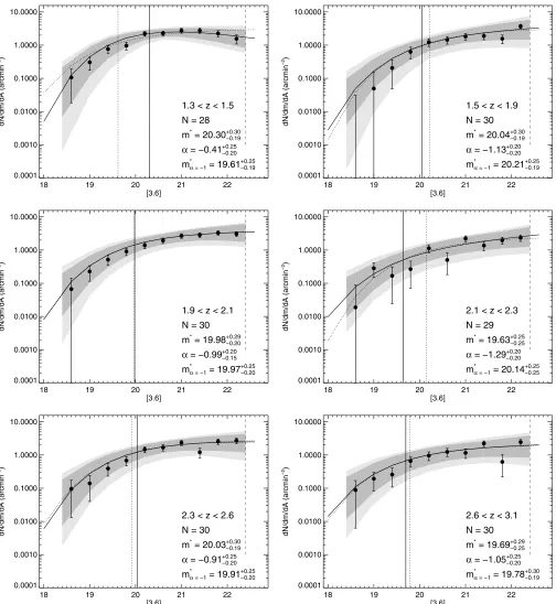
1 arcmin. Figure3shows the luminosity functions for CARLA
fields of richness2σdivided into six redshift bins.
The accurate measurement of the background number counts is essential for measuring the true cluster luminosity function. Because the SpUDS survey, used in this paper, covers only
∼1 deg2, it needs to be confirmed that it represents a typical
blank field and is not significantly affected by cosmic variance. At the depth of the CARLA observations, however, it is the largest contiguous survey accessible.
The 18 deg2 Spitzer Extragalactic Representative Volume
Survey (SERVS; Mauduit et al. 2012) reaches almost the
same depth as CARLA and allows a test of the goodness of SpUDS as a blank field. SERVS maps five well-observed astronomical fields (ELAIS-N1, ELAIS-S1, Lockman Hole,
Chandra Deep Field South, andXMM-LSS) with IRAC1 and
IRAC2. Coverage is not completely uniform across the fields but
averages∼1400 s of exposure time. We extracted sources from
the SERVS images (M. Lacy 2013, private communication) in the same way as we did for CARLA and SpUDS to allow for a
consistent comparison. In Figure4, we show the IRAC2 number
counts in SpUDS and SERVS observations of the XMM-LSS
field, illustrating the difference in depths of the two surveys. Comparing the SERVS number counts with the SpUDS number
counts gives an IRAC2 95% completeness limit of 2.85μJy for
the SERVS observations. As we aim to go as deep as possible for the CARLA analysis, the SERVS 95% completeness is slightly
shallow compared to the corresponding depth of 2.55μJy for
the CARLA observations. We therefore use the smaller area SpUDS survey for the background determinations.
To test the validity of our background subtraction, we placed
200 random apertures onto the 18 deg2 SERVS survey and
measured the density of IRAC-selected sources in those random cells. There is a chance that a CARLA cluster field and a non-associated large-scale structure are found in projection. In this case, our background subtraction would underestimate the
actual background in that field. By placing 200 random apertures
onto the 18 deg2SERVS survey, we can get a qualitative upper
limit of this probability. Figure 5 shows the distribution of
densities of IRAC-selected sources in those 200 random cells at the magnitude limit of the SERVS survey and compares it
to the distribution in SpUDS. SpUDS only covers ∼1 deg2
and is known to be biased to contain clusters and large-scale structure. The apertures placed on SpUDS cover almost the full area and will thus pick up any large-scale structure or clusters in that field. That is why a prominent high-density tail arises. By placing random apertures onto a larger survey that is less biased by large-scale structure, the high-density tail becomes less prominent, as expected.
To make sure, however, that we do not underestimate the background luminosity function by not taking enough of the high-density tail into account, we test here what impact our choice of background has on the overall results in this work. We repeat the luminosity function fitting analysis by choosing different density intervals to estimate the background, namely,
ΣSpUDS±0.8×σSpUDSandΣSpUDS±1.6×σSpUDS. Taking an
even narrower interval than ΣSpUDS±0.8×σSpUDS gives too
few apertures and results in a very noisy background luminosity
function. In Figure6, we show that the results for the luminosity
function fits with a fixedαfor the original background
subtrac-tion (1σ) and for the test background subtractions (0.8σ,1.6σ). The results for the different runs agree remarkably well and no
systematic effect is seen. AtΣSpUDS=ΣSpUDS±1.6×σSpUDS,
we are already sampling part of the high-density tail. Table2
shows that this has a minimal impact on the Schechter function fits. The exact choice of the density interval of the background subtraction is not critical and illustrates that choosing SpUDS
cells withΣSpUDS±σSpUDSis a sensible measure for the blank
field density of IRAC-selected sources.
3.3. Fitting Details
We make use of the Levenberg–Marquardt technique to solve the least-squares problem and to find the best solution form∗,α,
andΦ∗using the parameterization given in Equation (3). This
method is known to be very robust and to converge even when poor initial parameters are given. However, it only finds local minima. In order to find the true global minimum and the true best Schechter fit to our data, we vary the starting parameters and choose the best fit solution. We show the Schechter fits for
the CARLA fields of richness2σin Figure3.
Our data are deep enough to not just fit form∗ andΦ∗ and
assume a fixedαas had to be done in previous studies but to fit
for all three quantities,α,m∗andΦ∗simultaneously. Mancone
et al. (2012) shows thatα= −1 fits the galaxy cluster luminosity function at 1< z <1.5 well and that it stays relatively constant
down toz∼0. We therefore also repeat the Schechter fits with
fixedα= −1 (Table2).
3.4. Uncertainty and Confidence Region Computation
We estimate the uncertainties of the fitted parameters and the confidence regions of our fits using a Markov Chain Monte Carlo
(MCMC) simulation. Figure7shows the 1σ and 2σ contours
forαandm∗and the best Schechter fit.
We test our MCMC simulation by choosing a random set of
Φ∗,α, andm∗and by computingΦ
iatmifollowing Equation (3).
We then add normally distributed uncertainties ΔΦi so that
Φi,err = Φi +ΔΦi, and we fit a Schechter function toΦi,err.
18 19 20 21 22 23 [4.5]
0.0001 0.0010 0.0100 0.1000 1.0000 10.0000
Φ
= dN/dm/dA (arcmin
−2
)
1.3 < z < 1.5 N = 28 m*
= 19.83+0.29 −0.20 α = −1.00+0.15
−0.10
m*
α = −1 = 19.84
+0.20 −0.15
18 19 20 21 22 23
[4.5] 0.0001
0.0010 0.0100 0.1000 1.0000 10.0000
Φ
= dN/dm/dA (arcmin
−2
)
1.5 < z < 1.9 N = 30 m*
= 20.22+0.29 −0.20 α = −1.06+0.15
−0.15
m*
α = −1 = 20.31
+0.20 −0.15
18 19 20 21 22 23
[4.5] 0.0001
0.0010 0.0100 0.1000 1.0000 10.0000
Φ
= dN/dm/dA (arcmin
−2
)
1.9 < z < 2.1 N = 30 m*
= 20.18+0.25 −0.19 α = −0.92+0.15−0.10
m*α = −1 = 20.07
+0.15 −0.15
18 19 20 21 22 23
[4.5] 0.0001
0.0010 0.0100 0.1000 1.0000 10.0000
Φ
= dN/dm/dA (arcmin
−2
)
2.1 < z < 2.3 N = 30 m*
= 19.90+0.25 −0.25 α = −1.27+0.15−0.15
m*α = −1 = 20.40
+0.20 −0.15
18 19 20 21 22 23
[4.5] 0.0001
0.0010 0.0100 0.1000 1.0000 10.0000
Φ
= dN/dm/dA (arcmin
−2
)
2.3 < z < 2.6 N = 30 m* = 19.95+0.30−0.25 α = −1.09+0.15−0.15
m*
α = −1 = 20.09
+0.19 −0.15
18 19 20 21 22 23
[4.5] 0.0001
0.0010 0.0100 0.1000 1.0000 10.0000
Φ
= dN/dm/dA (arcmin
−2
)
2.6 < z < 3.1 N = 30 m* = 19.59+0.25−0.25 α = −1.28+0.15−0.10
m*
α = −1 = 20.09
[image:6.612.53.562.54.595.2]+0.20 −0.15
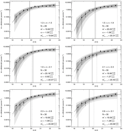
Figure 3.Schechter function fits to the 4.5μm cluster luminosity function in each redshift bin for CARLA cluster members withΣCARLA>2σ. The redshift bins
were chosen to contain similar numbers of objects,N. The solid circles are the binned differences between the luminosity function for all IRAC-selected sources in the clusters and the background luminosity function derived from the SpUDS survey. The solid curve shows the fit to the data for a freeα, while the dotted curve shows the fit forα= −1. The vertical solid and dotted lines show the fitted values form∗for free and fixedα, respectively. The dark and light gray shaded regions show the 1σand 2σconfidence regions for theα-free-fit derived from Markov Chain Monte Carlo simulations. The vertical dashed line shows the apparent magnitude limit. Note that due to binning of the data and the application ofk- ande-corrections, which are largest for the low-redshift LFs, we show the 99% magnitude limit here.
data pointsΦi,errand the Schechter fit agree very well with the
1 and 2σconfidence regions derived from the MCMC simulation
and prove that the MCMC simulation provides us with a proper
description of the uncertainties. Figure3shows the results of the
Schechter fits to the CARLA clusters withΣCARLA >2σfor all
redshift bins and the confidence regions derived from MCMC simulations.
4. ROBUSTNESS TESTS
4.1. Stability of the IRAC Color Criterion with Redshift
The evolution of the [3.6]−[4.5] color is very steep at
1.3 < z < 1.7; cluster members in our lowest redshift bin
are expected to have bluer colors, i.e., closer to −0.1, than
0.1 1.0 10.0
IRAC2 (μJy)
1000 10000
number counts (deg
−2
μ
Jy
−1
)
25 24 [4.5] 23
[image:7.612.318.568.54.238.2]SERVS SpUDS
Figure 4.Number counts for the SpUDS and SERVS survey for sources detected at 4.5μm. The 95% completeness limit of SERVS is derived by comparing the SERVS number counts to those from the SpUDS survey, which gives a completeness limit of 2.85μJy for IRAC2, as shown by the vertical dotted line. (A color version of this figure is available in the online journal.)
0 5 10 15 20
density (arcmin−2 ) 0.00
0.05 0.10 0.15 0.20
percentage of fields
[image:7.612.50.289.61.252.2]SERVS SpUDS
Figure 5.Distribution of IRAC-selected sources in the SpUDS and SERVS surveys. The apertures placed on SpUDS cover almost the full area of SpUDS and will pick up any cluster or large-scale structure in that field. By placing apertures onto the much wider SERVS survey that is less biased by large-scale structure the high-density tail becomes less prominent, as expected. This motivates us to use the SpUDS cells withΣSpUDS±σSpUDSas a sensible measure
of the blank field density of IRAC-selected sources.
(A color version of this figure is available in the online journal.)
a larger color uncertainty would therefore be expected to pass the criterion in some cases and not pass the criterion in other
cases. For the contaminating background/foreground sources,
this scattering is expected to be the same at all cluster redshifts. We therefore test if this effect has a statistically significant in-fluence on the faint end of the luminosity function in the lowest
redshift bin. Figure8shows the normalized number difference
between sources where [3.6]−[4.5] > −0.1 but [3.6]−
[4.5]-σ[3.6]–[4.5] <−0.1 and sources where [3.6]−[4.5]<−0.1 but
[3.6]−[4.5]+σ[3.6]–[4.5] > −0.1. In the following, we refer to
these sources as “scatter-in sources” and “scatter-out sources,” respectively. As the sum of the background and foreground color distribution is not expected to be dependent on cluster redshift and will therefore be the same for all redshift bins, any evolution in the difference between “scatter-in” and “scatter-out” sources
will be caused by the cluster members. As Figure8shows, the
19.8 20.0 20.2 20.4 20.6
[4.5]
> 2 σ 2.5−3.5σ > 3.5 σ
CARLA overdensity
α = −1 (1 σ BG suraction)
α = −1 (1.6 σ BG subtraction)
[image:7.612.49.289.312.478.2]α = −1 (0.8 σ BG subtraction)
Figure 6.Median best-fitm∗4.5withα= −1 as a function of galaxy cluster candidate richness for three different background-subtraction intervals. This demonstrates that the exact prescription of the background interval has an insignificant effect on the derived parameters. For clarity, data points for each background interval are shifted slightly along the horizontal axis.
(A color version of this figure is available in the online journal.)
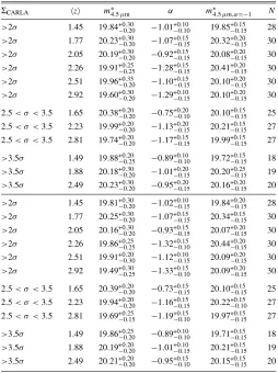
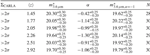
Table 2
Schechter Fit Results for BothαFree andαFixed to −1 to the 4.5μm Luminosity Function
ΣCARLA z m∗4.5μm α m∗4.5μm,α=−1 N
>2σ 1.45 19.84+0.30
−0.20 −1.01+0−0..1010 19.85+0−0..1515 28 >2σ 1.77 20.23+0.30
−0.20 −1.07+0−0..1515 20.32+0−0..2015 30 >2σ 2.05 20.19+0−0..3020 −0.92+0−0..1515 20.08
+0.20
−0.15 30 >2σ 2.26 19.91+0.25
−0.25 −1.28+0−0..1515 20.41+0−0..2015 30 >2σ 2.51 19.96−+00..3520 −1.10−+00..1515 20.10+0−0..2015 30 >2σ 2.92 19.60+0.30
−0.20 −1.29+0−0..1015 20.10+0−0..2015 30
2.5< σ <3.5 1.65 20.38+0−0..2020 −0.75+0−0..2010 20.10+0−0..1515 25 2.5< σ <3.5 2.23 19.99+0.20
−0.20 −1.13+0−0..2015 20.21+0−0..1515 27
2.5< σ <3.5 2.81 19.74+0−0..2020 −1.17+0−0..1515 19.99+0−0..1515 27 >3.5σ 1.49 19.88+0.20
−0.25 −0.89 +0.10
−0.10 19.72+0−0..1515 18 >3.5σ 1.88 20.18+0.30
−0.20 −1.01+0−0..2015 20.20+0−0..2515 19 >3.5σ 2.49 20.23+0.30
−0.20 −0.95+0−0..2015 20.16+0−0..2015 20 >2σ 1.45 19.81−+00..3020 −1.02−+00..1015 19.84+0−0..2015 28 >2σ 1.77 20.25+0.30
−0.20 −1.07−+00..1515 20.34 +0.15
−0.15 30 >2σ 2.05 20.16+0.30
−0.20 −0.93+0−0..1515 20.07+0−0..2015 30 >2σ 2.26 19.86−+00..2525 −1.32−+00..1510 20.44+0−0..2015 30 >2σ 2.51 19.91+0.20
−0.30 −1.12+0−0..1015 20.09+0−0..2015 30 >2σ 2.92 19.49−+00..3025 −1.33−+00..1510 20.09+0−0..2015 30
2.5< σ <3.5 1.65 20.39+0.20
−0.20 −0.73+0−0..1515 20.10+0−0..1515 25
2.5< σ <3.5 2.23 19.94+0−0..2020 −1.16+0−0..1515 20.22+0−0..1510 27 2.5< σ <3.5 2.81 19.69+0.25
−0.15 −1.19+0−0..1510 19.97+0−0..1515 27 >3.5σ 1.49 19.86−+00..2520 −0.89−+00..1010 19.71+0−0..1515 18 >3.5σ 1.88 20.19+0.20
−0.20 −1.01−+00..1015 20.21 +0.15
−0.15 19 >3.5σ 2.49 20.21+0.20
−0.20 −0.95+0−0..1510 20.15+0−0..1515 20
Notes.Below the horizontal line, we also show Schechter fit results for the same analysis but taking SpUDS cellsΣSpUDS=ΣSpUDS±1.6×σSpUDSto estimate
[image:7.612.317.571.366.706.2]19.0 19.5 20.0 20.5 21.0 21.5 [4.5]
−1.5 −1.0 −0.5 0.0
α
1σ
2σ
2σ
1.3 < z < 1.5 m* = 19.83+0.29−0.20 α = −1.00+0.15
−0.10
m*α = −1 = 19.84
+0.20 −0.15
N = 28
19.0 19.5 20.0 20.5 21.0 21.5
[4.5] −1.5
−1.0 −0.5 0.0
α
1σ
2σ
2σ
1σ
2σ
2σ
1.5 < z < 1.9 m* = 20.22+0.29−0.20 α = −1.06+0.15
−0.15
m*α = −1 = 20.31
+0.20 −0.15
N = 30
19.0 19.5 20.0 20.5 21.0 21.5
[4.5] −1.5
−1.0 −0.5 0.0
α
1σ
2σ
2σ
1σ
2σ
2σ
1.9 < z < 2.1 m* = 20.18+0.25−0.19 α = −0.92+0.15
−0.10
m*α = −1 = 20.07
+0.15 −0.15
N = 30
19.0 19.5 20.0 20.5 21.0 21.5
[4.5] −1.5
−1.0 −0.5 0.0
α
1σ
2σ
2σ
1σ
2σ
2σ
2.1 < z < 2.3 m* = 19.90+0.25−0.25 α = −1.27+0.15
−0.15
m*α = −1 = 20.40
+0.20 −0.15
N = 30
19.0 19.5 20.0 20.5 21.0 21.5
[4.5] −1.5
−1.0 −0.5 0.0
α
1σ
2σ
2σ
1
σ
2σ
2σ
2.3 < z < 2.6 m* = 19.95+0.30−0.25 α = −1.09+0.15
−0.15
m*α = −1 = 20.09
+0.19 −0.15
N = 30
19.0 19.5 20.0 20.5 21.0 21.5
[4.5] −1.5
−1.0 −0.5 0.0
α
1σ
2σ
2σ
1σ
2σ
2σ
2.6 < z < 3.1 m* = 19.59+0.25−0.25 α = −1.28+0.15
−0.10
m*α = −1 = 20.09
+0.20 −0.15
[image:8.612.62.549.57.598.2]N = 30
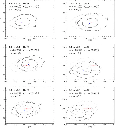
Figure 7.Confidence regions forαvs.m∗for Schechter fits withαas a free parameter derived from the Markov Chain Monte Carlo simulations. The contours show the 1σand 2σcontour levels and the blue solid circle shows the result of the best Schechter fit using the Levenberg–Marquart technique. The redshift bins were chosen to contain similar numbers of objects,N. The red solid circle with uncertainty onm∗shows the best Schechter fit for a fixedα= −1. In all cases, the results from the fixedαfit and the freeαfit agree within their confidence regions implying thatα= −1 describes the luminosity function well over the whole redshift range probed in this work. For comparison, we show the lowest redshift contours (dotted gray) in the higher redshift panels.
(A color version of this figure is available in the online journal.)
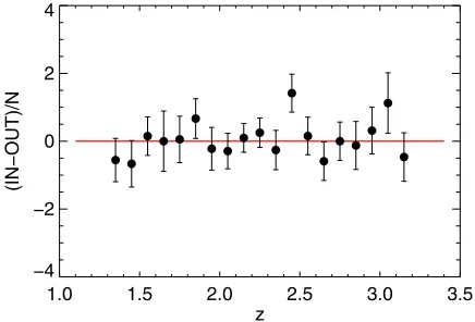
evolution of the difference is consistent with being flat with redshift. The mean of the distribution is 0.06 (Nfields)−1 and a
Spearman rank correlation analysis only gives a 33% chance that there is an evolution of the difference with redshift. This test confirms that the color selection is very efficient and stable with redshift and that statistically the same portion of cluster members is selected at all redshifts.
4.2. Validation of the Luminosity Function Measurement Method Using ISCS Clusters
We use the ISCS (Eisenhardt et al. 2008) to validate the
methodology used in this paper and to compare to previously
obtained results. Mancone et al. (2010) uses the ISCS to
1.0 1.5 2.0 2.5 3.0 3.5 z
−4 −2 0 2 4
[image:9.612.59.277.56.204.2](IN−OUT)/N
Figure 8.Average number of sources that could scatter in or out of the IRAC color selection due to photometric uncertainties as a function of candidate cluster redshift. “IN” are defined as sources currently not selected (e.g., [3.6]–[4.5] < −0.1) but which could easily scatter in due to photometric uncertainties, [3.6]–[4.5]+σ[3.6]–[4.5]>−0.1. “OUT” are defined as currently selected sources (e.g., [3.6]–[4.5]>−0.1) but which could easily scatter out due to photometric uncertainties, [3.6]–[4.5]−σ[3.6]–[4.5]<−0.1. The results are relatively flat and centered at zero, implying that the color criterion used is efficient and stable at all redshifts probed here.
(A color version of this figure is available in the online journal.)
candidate cluster members based on photometric redshifts,
com-puted as in Brodwin et al. (2006) and with deeper photometry
from the Spitzer Deep, Wide-Field Survey (SDWFS; Ashby
et al.2009). We measure the luminosity function around ISCS
clusters at 1.3< z <1.6 and 1.6< z <2, i.e., overlapping in redshift with the CARLA cluster sample. We again first apply
the IRAC color criterion to the sources in a cell with radiusr=
1 arcmin around the cluster center to determine cluster member candidates and carry out a background subtraction using SpUDS as described above. We then fit a Schechter function to the
re-sulting data withαfixed to−1. The SDWFS data is shallower
than CARLA, and we can therefore only measure the luminosity function down to [4.5]=21.4. The fitted values form∗at 4.5μm are 20.25+0−0..3030and 20.57+0
.35
−0.35for clusters at 1.3< z <1.6 and
1.6 < z < 2, respectively. Them∗ for the same redshift bins
andα = −1 found by Mancone et al. (2010) are 20.48+0−0..1209
and 20.71+0.18
−0.12. Our results agree very well with these values,
though please note the larger error bars inherent to our simple color selection compared to the photometric redshift selection
of Mancone et al. (2010), which minimizes background
contam-ination by incorporating extensive multi-wavelength supporting data. This test confirms that the method used in this paper, i.e., color-selecting galaxy cluster members and carrying out a sta-tistical background subtraction, provides robust results. With this test, we also confirm the trend toward fainter magnitudes
form∗in ISCS clusters in the highest redshift bins reported by
Mancone et al. (2010).
5. THE REDSHIFT EVOLUTION OF M∗
5.1. Comparison to Galaxy Evolution Models
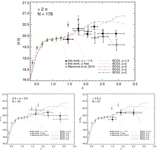
Figure9shows the evolution ofm∗with redshift in the context
of passively evolving stellar population models. We also include
results from Mancone et al. (2010). The measuredm∗ values
are compared to previous work and to model predictions of passively evolving stellar populations from Bruzual & Charlot
(2003) normalized to match the observedm∗of galaxy clusters
atz∼0.82, [4.5]∗ =19.82+0.08
−0.08 (AB) forα = −1 (Mancone
et al.2012). Note that the results and implications of our work
are independent of the model normalization. Although Mancone
et al. (2010) used a normalization obtained from lower redshift
cluster analyses, we use a normalization at relatively high redshift to match the redshift of the CARLA data as best as possible.
Mancone et al. (2010) carried out a similar study and
measured the IRAC1 and IRAC2 luminosity function for 296
galaxy clusters from SDWFS over 0.3 < z < 2. The clusters
were identified as peaks in wavelet maps generated in narrow
bins of photometric redshift probabilities. At z < 1.3, the
evolution of m∗ agreed well with predictions from passively
evolving stellar populations and no mass assembly, with an
inferred formation redshift of zf = 2.4. For the two highest
redshift bins at z > 1.3, the results disagreed significantly
from the continuation of the passive evolution model. Mancone
et al. (2010) interpreted this deviation as possible ongoing mass
assembly at these epochs. The results here for the CARLA clusters do not agree with nor continue the trend Mancone et al. (2010) report atz >1.3. In the redshift bins in which our study
and Mancone et al. (2010) overlap, we findm∗to be∼0.5 mag
brighter and to continue the trend found at lower redshifts by Mancone et al. (2010). At lower redshift (1.3 < z <1.8), the
models do not differ much andm∗is therefore consistent with
a range of formation redshifts. At higher redshift, the models diverge and show that clusters may have formed early with formation redshifts in the range 3< zf <4.
At all redshifts, our results are consistent with passive
evolution models with 3 < zf < 4. As CARLA clusters at
z ∼3 will not necessarily be progenitors of CARLA clusters
atz∼1.5, it does not necessarily imply that they will remain
passive subsequently. However, even at the highest redshifts
probed here (z∼3), we do not measure a prominent deviation
from passive evolution models nor do we see signs of significant mass assembly.
5.2. Dependence on Cluster Richness
We also study the evolution of m∗ for two CARLA
sub-samples of different richnesses (2.5σ < ΣCARLA < 3.5σ and
ΣCARLA > 3.5σ) and plot the results in Figure9. Although it
is not fully known how the richness of IRAC-selected sources scales with mass, we assume here that statistically these two subsamples will represent clusters of increasing mass. For the
lower richness sample, the evolution ofm∗appears to be similar
to the full sample with formation redshifts of 3< zf <4.
Ex-cluding the highest and lowest richness clusters therefore does not seem to have a significant effect on the luminosity func-tions. At lower redshift (i.e., 1.3< z < 2.0) the result form∗
and freeαis consistent with results from Mancone et al. (2010)
atz1.3 which might suggest that the CARLA lower richness
clusters at this redshift are similar to the ISCS clusters studied
Mancone et al. (2010).
Only considering the highest richness sample of CARLA
clusters results in a monotonically increasingm∗, withm∗ ∼
0.7 mag fainter in the highest redshift bin compared to the lower richness samples. This might imply that the high richness sample includes slightly older stellar populations. This subsample is thus of particular interest for future follow-up as this population of rich, high-redshift clusters could provide a powerful probe to study the early formation of massive galaxies in the richest environments and—from a cosmological point of view—test the
0.5
1.0
1.5
2.0
2.5
3.0
3.5
z
18.0
18.5
19.0
19.5
20.0
20.5
21.0
21.5
[4.5]
BC03, zf=1.5
BC03, zf=2
BC03, zf=3
BC03, zf=4
BC03, zf=5
this work, α = −1.0
this work, α free
Mancone et al.,2010
> 2
σ
N = 178
0.5 1.0 1.5 2.0 2.5 3.0 3.5
z 18.0
18.5 19.0 19.5 20.0 20.5 21.0 21.5
[4.5]
BC03, zf=1.5 BC03, zf=2 BC03, zf=3 BC03, zf=4 BC03, zf=5
this work, α = −1.0
this work, α free
Mancone et al.,2010 2.5 < σ < 3.5
N = 79
0.5 1.0 1.5 2.0 2.5 3.0 3.5
z 18.0
18.5 19.0 19.5 20.0 20.5 21.0 21.5
[4.5]
AB
BC03, zf=1.5 BC03, zf=2 BC03, zf=3 BC03, zf=4 BC03, zf=5
this work, α = −1.0
this work, α free
Mancone et al.,2010 > 3.5 σ
[image:10.612.58.564.54.536.2]N = 57
Figure 9.Evolution ofm∗4.5μmwith redshift for different CARLA cluster densities compared with results from Mancone et al. (2010) and model predictions for passive stellar population evolution (Bruzual & Charlot2003) with different formation redshifts,zf. The number of CARLA fields going into each analysis is indicated on the plots. In most cases, the results for the Schechter fits with fixedαand freeαagree well. In cases where they do not, this is due to bigger uncertainties at the faint end of the luminosity function in the data. In these cases, the fixedαfit is probably the more meaningful result as it has been shown that generally a faint end slope ofα= −1 describes the data well at all CARLA densities and all redshifts. In general, our results are consistent with the passive evolution models out toz∼3 with formation redshifts 3< zf <4. The lower-density CARLA sample, shown in the lower left panel, seems to be consistent with results from Mancone et al. (2012) atz1.3 and suggests that this CARLA subsample is similar to the clusters studied there. The high-density subsample of CARLA clusters, shown in the lower right panel, are∼0.7 mag fainter in the highest redshift bin compared to the lower richness samples. This might imply that the high richness sample consists of older clusters and therefore could provide a valuable sample of high-richness high-redshift clusters to study the formation of the earliest massive galaxies. For clarity, the results for a fixedαare slightly shifted along thex-axis.
(A color version of this figure is available in the online journal.)
5.3. Difference betweenα=free andα= −1 Fits
As can be seen in Figures7 and9, the Schechter fit results
for α as a free parameter andα fixed to −1 generally agree
well within the 1σ uncertainties. For the few exceptions, the
fits do agree within the 2σ uncertainties. We conclude that a
fixedαof−1 describes the luminosity function functions well
at all redshifts and all densities probed in this paper. With deeper
IRAC observations (1400 s of exposure time), albeit not as deep as the CARLA observations (2000 s of exposure time) and deep
multi-wavelength supporting data, Mancone et al. (2012) study
a subset of the original B¨ootes sample and measure the faint
end slope αof the mid-IR galaxy cluster luminosity function
to be∼−1 at 1 < z < 1.5. Similar studies at lower redshift
measure similar slopes. This suggests that the shape of the
The luminosity functions measured in this paper are
con-sistent withα= −1 at all redshifts and all richnesses probed.
Combined with results from Mancone et al. (2010) and Mancone
et al. (2012), this result suggests that galaxy clusters studied in this paper have already started to assemble low-mass galaxies at early epochs. Further processes that govern the build up of
the cluster and that are discussed in more detail in Section6
then have probably no net effect on the shape of the luminosity function. This is consistent with the results found by Mancone et al. (2010).
6. DISCUSSION
6.1. Alternatives to Pure Passive Evolution Models
The above results suggest an early formation epoch for galaxy clusters that are passively evolving and an early build-up of the low-mass galaxy population. These measurements, however, seem to be at odds with results investigating lower redshift
clusters. Thomas et al. (2010) shows that the age distribution
in high-density environments is bimodal with a strong peak at
old ages and a secondary peak composed of young,∼2.5 Gyr
old galaxies. This secondary peak contains about∼10% of the
objects. Similarly, Nelan et al. (2005) derives a mean age of
low-mass objects of low redshift galaxy clusters to be about 4 Gyr in low-redshift clusters. Although their observation suggests a decline of star-forming galaxies and a trend of downsized galaxy formation, low mass galaxies are still assembling until relatively recent times. Measurements of the star-formation activity for higher redshift cluster galaxies also provide evidence for continuous star-formation activity, albeit evolving more rapidly than the star-formation activity in field galaxies (Alberts et al.2014, e.g.,).
We therefore investigate the extent to which our results can be explained by a sum of various stellar populations to estimate the maximum fraction of a star-forming cluster population that is still consistent with the data. We divide the cluster population into two stellar populations, a simple stellar population (SSP) with a delta-burst of star formation at high redshift and a composite stellar population (CSP) with a continuous, only slowly decaying star-formation rate (SFR) of
the form ∝ exp(−t /τ) and large τ. The details of the three
different model sets we derive are as follows.
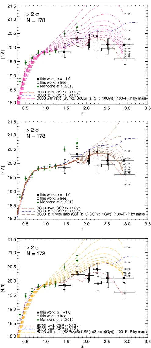
1. Model 1. Sum of SSP withzf =3 and CSP withzf =3
andτ = 10 Gyr with ratios (SSP:CSP) ranging between
90:10 and 0:10012by mass.
2. Model 2. Sum of SSP withzf =3 and CSP withzf =3
andτ = 1 Gyr with ratios (SSP:CSP) ranging between
90:10 and 0:100 by mass.
3. Model 3. Sum of SSP withzf =5 and CSP withzf =3
andτ = 10 Gyr with ratios (SSP:CSP) ranging between
90:10 and 0:100 by mass.
A prolonged mass assembly means that at high redshift the
observed 4.5μm magnitude of galaxies is fainter because the
stellar population is still forming. Therefore, accounting for mass assembly, i.e., allowing for star-forming population to
contribute to the observedm∗, causesm∗ to become fainter at
high redshift depending on the contribution of this star-forming population.
12 A ratio (SSP:CSP) of (100:0) is equivalent with a passive evolution model
and is already discussed above.
In Figure 10, we show these models in the context of our
results. They allow us to set an upper limit on the star-forming
fraction, P, in our candidate cluster sample. Model 1, which
allows for a significant star formation that is only very slowly decaying with cosmic time, shows that at all redshifts the mass fraction of the star-forming population cannot be larger than
40% (with one outlying exception of up to 60% atz∼1.7). In
Model 2, the SFR of the CSP decays faster and the contribution of the SSP becomes dominant much earlier than in Model 1.
It therefore predicts m∗ to be brighter at high redshifts and
to resemble the prediction of the passive evolution model. Consequently, our empirical results are in agreement with large contributions of up to 90% of the CSP in Model 2, with the CSP starting to passively evolve∼2.3 Gyr earlier (atz∼1.7) than in
Model 1 (atz∼0.9). Model 3 shows the evolution of a mixed
population with a delta burst of star formation atzf =5 (SSP)
and a long burst of star formation atzf =3 (CSP withτ =10
Gyr). The SSP withzf =5 is fainter in IRAC2 at 1.5< z <3
than an SSP withzf =3, so that an additional starburst atz=3
leads to an even fainterm∗at 1< z <3 for Model 3. Model 3
does not reproduce the results of the LF analysis, and therefore, this scenario can be ruled out by the data.
This shows that the results for the evolution ofm∗obtained
in this analysis—although consistent with passive evolution models—also allow for a limited contribution of a star-forming population in galaxy clusters. Our models show that this contribution is small (up to 40% by mass, but probably on
average around∼20%) for a population with a high and slowly
decaying SFR, or that this contribution is large (up to 80%) for a population with a fast decaying SFR and an evolution that
resembles passive evolution∼2.3 Gyr earlier.
For a sample of 10 rich clusters at 0.86< z <1.34, van der
Burg et al. (2013) compares the contributions of quiescent and
star-forming populations to the total mass function. We integrate the published mass functions for the quiescent and star-forming
population (van der Burg et al.2013) over galaxy masses with
1010.1 < M∗/M < 1011.5. We find a mass fraction of the
quiescent population of ∼80% compared to the total stellar
mass of the clusters. This is also in agreement with the upper limit for the fraction of the star-forming population derived for CARLA clusters in the lowest redshift bin.
As CARLA clusters at z ∼ 3 will not necessarily be the
progenitors of CARLA clusters atz ∼ 1.5, we unfortunately
cannot constrain the evolution of the maximum fraction of a star-forming population and cannot make conclusions about the quenching timescales and processes.
6.2. Biases of the CARLA Cluster Sample
Our analysis shows that the evolution of the CARLA clusters seems to be significantly different from the cluster sample
analyzed by Mancone et al. (2010). Using Spitzer 24 μm
imaging for the same cluster sample, Brodwin et al. (2013)
analyzed the obscured star formation as a function of redshift, stellar mass, and clustercentric radius. They find that the transition period between the era where cluster galaxies are significantly quenched relative to the field and the era where
the SFR is similar to that of field galaxies occurs at z∼ 1.4.
Combining these measurements with other independent results
on that sample (Snyder et al.2012; Martini et al.2013; Alberts
et al.2014), the authors conclude that major mergers contribute
significantly to the observed star formation history and that merger-fueled AGN feedback may be responsible for the rapid
0.5 1.0 1.5 2.0 2.5 3.0 3.5 z
18.0 18.5 19.0 19.5 20.0 20.5 21.0 21.5
[4.5]
P = 90
P = 80
P = 70 P = 60 P = 50 P = 40 P = 30 P = 20 P = 10
this work, α = −1.0
this work, α free
Mancone et al.,2010
BC03 with ratio (SSP(zf=3):CSP(zf=3,τ=10Gyr)) (100−P):P by mass
BC03, zf=5, CSP τ=0.1Gyr
BC03, zf=3, CSP τ=0.1Gyr
> 2 σ N = 178
0.5 1.0 1.5 2.0 2.5 3.0 3.5
z 18.0
18.5 19.0 19.5 20.0 20.5 21.0 21.5
[4.5]
P = 90
P = 80
P = 70 P = 60 P = 50 P = 40 P = 30 P = 20 P = 10
this work, α = −1.0
this work, α free
Mancone et al.,2010
BC03, zf=3 with ratio (SSP(zf=3):CSP(τ=1Gyr)) (100−P):P by mass
BC03, zf=5, CSP τ=0.1Gyr
BC03, zf=3, CSP τ=0.1Gyr
> 2 σ N = 178
0.5 1.0 1.5 2.0 2.5 3.0 3.5
z 18.0
18.5 19.0 19.5 20.0 20.5 21.0 21.5
[4.5]
P = 10
P = 90
P = 80
P = 70 P = 60 P = 50 P = 40 P = 30 P = 20 P = 10
this work, α = −1.0
this work, α free
Mancone et al.,2010
BC03 with ratio (SSP(zf=5):CSP(zf=3,τ=10Gyr)) (100−P):P by mass
BC03, zf=5, CSP τ=0.1Gyr
BC03, zf=3, CSP τ=0.1Gyr
[image:12.612.45.292.50.616.2]> 2 σ N = 178
Figure 10. Model predictions for the evolution ofm∗ for a superposition of a passive and star-forming galaxy population. The passive, simple stellar population (SSP) formed stars in a delta burst atzf and evolved passively thereafter while the star-forming, composite stellar population (CSP) shows an exponentially decaying SFR with ane-folding timescaleτ. We show models with differing mass ratios of the SSP and CSP. Comparing the models with our measurements form∗allows us to set an upper limit on the contribution of the CSP. Top panel: Model 1: SSP withzf =3, CSP withzf=3 andτ=10 Gyr. Middle panel: Model 2: SSP withzf =3, CSP withzf =3 andτ =1 Gyr. Bottom panel: Model 3: SSP withzf=5, CSP withzf=3 andτ=10 Gyr. (A color version of this figure is available in the online journal.)
While the ISCS clusters studied in Mancone et al. (2010) and
Brodwin et al. (2013) were selected from a field survey as
three-dimensional overdensities using a photometric redshift wavelet analysis, the clusters studied here are found in the vicinity of RLAGN. With RLAGN belonging to the most massive galaxies in the universe (m∼1011.5M
; Seymour et al.2007; De Breuck
et al.2010), these clusters could reside in the largest dark matter halos, deepest potential wells, and densest environments.
Indeed, Mandelbaum et al. (2009) derives halo masses for
5700 RLAGN from the Data Release 4 of the Sloan Digital Sky Survey and finds the halo masses of these RLAGN to be about twice as massive as those of control galaxies of the same stellar
mass. Previous work (e.g., Best et al.2005)has shown that more
massive black holes seem to trigger radio jets more easily, but as this boost in halo mass is independent of radio luminosity, the authors conclude that the larger-scale environment of the RLAGN must play a crucial role for the RLAGN phenomenon. Similarly, albeit at higher redshift, N. A. Hatch et al. (in preparation) finds that the environments of CARLA RLAGN are significantly denser than similarly massive quiescent galaxies. They detect a weak positive correlation between the black-hole mass and the environmental density on Mpc-scales, suggesting that even at high redshift the growth of the black hole is also linked to collapse of the surrounding cluster.
This peculiar interplay between radio jet triggering, stellar mass, black hole, and halo mass of the RLAGN and the larger-scale environment suggest that (proto-)clusters and the large-scale environments of RLAGN are distinct from clusters found in field surveys.
If mergers are significantly contributing to the transition of clusters from unquenched to quenched systems, as suggested in
Brodwin et al. (2013), this transition redshift will be dependent
on cluster halo mass. If the environments and dark matter halos around RLAGN are indeed more massive this would explain the
conflict of our results with those from Mancone et al. (2010).
CARLA clusters have probably undergone this transition period much earlier than the ISCS clusters. At 1.4 < z < 1.8 where the star-forming fraction of ISCS clusters analyzed by Mancone et al. (2010) still seems to be very high (∼80%), this contribution is already much smaller in CARLA clusters. As mentioned earlier, our measurements allow us to derive upper limits on the contribution of a star-forming population but do not allow for a definite constraint on the transition redshift.
7. SUMMARY
We have shown the evolution of the mid-IR luminosity function for a large sample of galaxy cluster candidates at
1.3< z < 3.2 located around RLAGN. All cluster candidates
in this work were identified as mid-IR color-selected galaxy overdensities, a selection that is independent of galaxy type
and evolutionary stage. Wylezalek et al. (2013) has shown that
indeed these excess color-selected sources are centered on the RLAGN, implying they are associated. There is a steep increase of density toward the RLAGN which would not be seen if there was not a physical link between the galaxies in the field and the AGN. We therefore expect most of these overdensities to be true galaxy (proto)-clusters. Having neither spectroscopic nor photometric redshifts at hand, this study relies on statistics with 10–30 clusters per redshift bin.
We have shown that our results are consistent with theoretical
passive galaxy evolution models up toz=3.2. Mancone et al.