Best Response Games on Regular Graphs

http://dx.doi.org/10.4236/am.2013.46131 Published Online June 2013 (http://www.scirp.org/journal/am)

Best Response Games on Regular Graphs

Richard Southwell, Chris Cannings

School of Mathematics and Statistics, University of Sheffield, Sheffield, UK Email: richardsouthwell254@gmail.com, c.cannings@sheffield.ac.uk Received March 8, 2013; revised April 10, 2013; accepted April 18, 2013

Copyright © 2013 Richard Southwell, Chris Cannings. This is an open access article distributed under the Creative Commons Attri-bution License, which permits unrestricted use, distriAttri-bution, and reproduction in any medium, provided the original work is properly cited.

ABSTRACT

With the growth of the internet it is becoming increasingly important to understand how the behaviour of players is af- fected by the topology of the network interconnecting them. Many models which involve networks of interacting play- ers have been proposed and best response games are amongst the simplest. In best response games each vertex simulta- neously updates to employ the best response to their current surroundings. We concentrate upon trying to understand the dynamics of best response games on regular graphs with many strategies. When more than two strategies are present highly complex dynamics can ensue. We focus upon trying to understand exactly how best response games on regular graphs sample from the space of possible cellular automata. To understand this issue we investigate convex divisions in high dimensional space and we prove that almost every division of k − 1 dimensional space into k convex regions in- cludes a single point where all regions meet. We then find connections between the convex geometry of best response games and the theory of alternating circuits on graphs. Exploiting these unexpected connections allows us to gain an interesting answer to our question of when cellular automata are best response games.

Keywords: Games on Graphs; Cellular Automata; Best Response Games; Social Networks

1. Introduction

Game theory is a rich subject which has become more diverse over the years. Early game theory [1] focused on how rational players would behave in strategic conflicts. Concepts like the Nash equilibrium [2] helped theorists to predict final outcomes of games, and this benefited areas like economics. A more recent development is evo- lutionary game theory [3]. Rather than assuming that players are hyper-rational, evolutionary game theory con- cerns itself with large populations of players that change their strategies via simple selection mechanisms. Players repeatedly engage in games with other members of the population and the way the populations strategies evolve depends upon the selection mechanism employed.

One way to introduce a spatial aspect into evolutionary games is to imagine the players as vertices within a graph [4,5]. The links represent interactions so vertices play games with their neighbours. The players adapt their stra- tegies over time to try to increase their success against neighbours. Many kinds of update rules have been inves- tigated. These include imitation, where vertices imitate their most successful neighbour, and best response, where vertices update to employ the strategy best suiting their current surroundings. In [6] the authors study a two-

dimensional cellular automata with update rules based upon games, beautiful patterns emerge.

In previous studies we investigated the dynamics of games on networks where the players update asynchro- nously [7-10] as they engage in congestion games (where an individual’s payoff decreases with the number of their neighbours using the same strategy). We have also inves- tigated more exotic scenarios, where the network struc- ture itself changes as a result of the strategic interactions between the players/vertices. These type of game based network dynamics can produce remarkably complex struc- tures despite being based upon extremely simple rules, involving reproducing vertices [11-14]. In some of these game based network growth systems, small initial net- works can lead to the creation of thousands of different structures which morph and self replicate in complex ways [15,16].

vertex updates to may not be optimal because neighbour- ing vertices change their strategies at the same time. Work on these kind of systems includes [17] and [18], where it was shown that a two strategy game running upon any graph will eventually reach a fixed point or pe- riod two orbit. Two strategy best response games on va- rious graph structures were also studied in [19].

The systems we consider are essentially cellular auto- mata with update rules that are induced by the details of the game. In our consideration of best response games on the circle we will see many of Wolfram’s 256 elementary cellular automata [20] appear. Under these models the states of the vertices on a circle or line graph take values in {0,1}. The states of vertices change with time so that the future state of any cell depends upon the current state of itself and its neigbours. Each systems is specified by a mapping f : 0,1

 

3

 

0,1 so that f x



i1, ,x xi i1



is the future state of a vertex in state xi with neighbours

in states xi1 and xi1 to its left and right. Each system is indexed with a number

































0 1 3 4 6 7

0,0,0 2 0,0,1 2 0,1,0 2 0,1,1 2 1,0,0 2 1,0,1 2 1,1,0 2 1,1,1 2

f f f

f f f

f f               2 5 



We concentrate upon games on the circle because they provide the easiest ways to illustrate our results. Our me- thods can easily be extended to other graph structures, even non-regular ones.

1.1. Definitions

For a set let to be the set of size multi sets of elements from i.e. is the set of all unordered -tuples

S d

 

d S  S d

 

d S  , d



s s1, ,2 

 

v

s

G V

S

of members of , including those -tuples containing more than one of the same element. Let us define a regular automata as a quad , where is a regular degree graph, is a set of states, is an assignment of a state

S d

 



G ,F



S 0  0 d , ,

G S 



,E





 

G 0

 to each vertex vV (the initial configuration) and : d

 

F  S S is the up- date function/rule.

Such a regular automata evolves so that at time step , the future state of a vertex , at time

0

t v t1, will

be

 









1

1, , ,2

t

d

v F s s s

 _{  (1.1)}

where



1, , ,2





 

 



t d

s s  s   u uNe v (1.2) is the set of states of vertices in ’s neighbourhood,

, at time .

v

 

Ne v t

,M

A game



consists of a set of strategies which we label with integers, together

with a







k



1, 2, ,

  

k k payoff matrix M such that Mi j, 

i

is the payoff that a player receives from employing the th strategy against the jth strategy.

The best response games we consider take place on a degree regular graph . At time t each

vertex d

v V



,E



G V

 employs a strategy t

 

v  . The total

payoff

  t u

e v  ,

t _v

 

u N



M (1.3)

of at time is the sum of payoffs that receives from using its strategy in a game with each neighboring player. At time each vertex simultaneously updates its strategy, so that at time it will employ the stra- tegy that would have maximised its total payoff, given what its neighbours played at time . In other words each player updates to play the best response to its cur- rent surroundings.

v t

v

t

1

t t

Best response games on regular graphs are quads

 



G, , 0 G ,M



, which are defined by a regular graph

G, a game



,M



and an assignment 0

 

G of an

initial strategy to 0

 

v  to each vertex of G. A

best response game is a regular automata

 



G, , 0 G ,F



with an update function F such that, for every unordered d-tuple of strategies



s s1, ,2 ,sd



 

d 



 , we have F





s s1, , ,2  sd





is

the strategy in



 



that maximises

,i 1 . d s i



M (1.4)

We refer to F as the update function induced by the game



,M



. Note that in rare cases the payoff matrix

could be such that two strategies are tied as best re- sponses to a possible local strategy configuration



s s1, ,2 ,sd



. In such a case F





s s1, , ,2  sd





1 ,vn



is not properly defined. Such a problem can always be allevi- ated by an infinitesimal perturbation of the elements in the payoff matrix . We always assume our matrix is such that this problem never occurs.

M

n

1.2. Examples on the Circle

The circle graph has vertices



0 1



with is adjacent to

C v v, ,

i

v v_j if and only if i j 1modn

 



C ,M



. Every best response game _{, ,} 0 on the

n n

C  

circle is a regular automata



_{, ,} 0

 

_,



, where

n n

C   C F

the strategy

 

i

1

t

v

 _{employed by vertex at time}

i

v 1

t will be





t



_{ 1mod }



t



_{ 1mod }







i n

v _

,

i n

 _ 

F v , which is

the strategy that maximises the vertices’s total payoff against its neighbours strategies



_ 1mod



and

t

i n

v

 _{ }

 



i 1modn



t

v

 _ .

1 0 4 2 M  



  (1.5) is a Hawk-Dove game, where 1 is the passive dove stra- tegy and 2 is the aggressive hawk strategy. Let us con- sider the best response game , where and M is as above. This corresponds

 



_{, ,} 0 _,



n n

C   C M

 



C ,F



 

1, 2

 

to the regular automata _{, ,} 0 with update

n n

C  

function F



 

1,1



2, and



1 F



 

1, 2



2

 



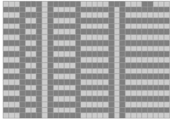
2, 2

F . We picture how this automata will evo- lves on a 30 vertex circle from a random strategy con- figuration, with the space time plot pictured in Figure 1.

A space time plot [20] is a grid where the x axis is the index of the vertex of the circle and the axis (reading downwards) is the time step. Light gray blocks denote employers of strategy 1 whilst dark blocks re- present employers of strategy 2. In our game a player ad- jacent to an employer of dove and employer of hawk gets updated to play the hawk strategy, hence if a block on our space time plot has a dark gray block on its left and a light gray block on its right then the block below it will be dark gray. The system corresponds to Wolfram’s cel- lular automata number 95, which is well known to have simple dynamics. Every initial configuration evolving quickly to a fixed point or period 2 orbit. This system is an example of a threshold game [17,18].

y

More complicated dynamics occur under the 3 strategy game with payoff matrix

3 94 46 33 85 66 , 52 2 67

 

  

 

 

M _ (1.6)

Figure 2 shows the evolution of the system from a

random initial configuration on a 60 vertex circle over 40 time steps. In this case dark gray, white and light gray blocks represent strategies 1, 2 and 3 respectively. The resulting cellular automata can be reduced to Wolfram’s cellular automata number 90 which has been proven to be chaotic [21] when running on an infinite circle.

In this paper we will enumerate all the update func- tions F that can be induced by 2, 3 or 4 strategy best

response games on the circle by consideration of the con- vex geometry behind best response game. Understanding this convex geometry allows one to understand how the update rules of arbitrary best response games are in- duced.

1.3. Overview

[image:3.595.338.506.85.203.2]

In Section 2 we discuss some important relationships between best response games and divisions of the sim- plex into convex regions. By using games on the circle as examples, we describe the relationships with convex di- visions, and then present Theorem 2.1, which is our key

Figure 1. A space time plot showing the evolution of the Hawk-Dove example game on the circle.

Figure 2. A space time plot showing the evolution of the three strategy game described by the payoff matrix in Equ- ation (1.6).

theoretical result.

In Section 3 we discuss how our theory of convex divisions can be used to find all the different best re- sponse games on the circle which have two or three strategies. We also describe the dynamics of the different two strategy games on the circle, and point out relation- ships with famous games.

In Section 4 we discuss how our theory can be ex- tended to games with more than three strategies. In parti- cular, we derive Theorem 4.3 which relates our problem of enumerating games on the circle with strategies to the theory of alternating cycles in graphs.

k

In Section 5 we discuss how our theory can be used to investigate the dynamics of best response games on more general types of graphs. In particular, we demonstrate how our game enumeration methods can easily be ex- tended to count the number of different games on generic regular graphs. We also explain how our results can be applied to non-regular graphs.

2. Convex Geometry behind Best Response

Games

For a game



,M



, let us think of each strategy



1, 2, ,



i  k as a unit vector

 

i 



 1,i, 2,i, ,k i,



k

e   , (1.7)

The strategy space is the convex hull of the set of unit strategy vectors. The points

k

 



x x1, , ,2 xk



x 



  (1.8)

are probability distributions over the set of strategies  so that xi is the fraction of the th strategy employed

in the strategy vector .

i

x

The affine hull of



e

 

i i



forms the extended strategy space S which we can write as



k_| T ₁

  

S x  x1



, (1.9)

where is the length vector with each entry equal to 1. Here

1 k

S is isomorphic to k1 and  S so

we think of as a dimensional unit simplex, with the unit strategy vectors as its vertices. For each pair of strategy vectors the payoff one receives from playing against is

 1

x

k

k e

 

i

, x y

y

S

T_.

xMy (1.10)

The best response set to any strategy vector xS is

the set of pure strategies such that i  j 

 

T

 

_.

i  j

e My e MyT (1.11)

The th best response region i is the set of all

points in

i R S

S that have a best response set equal to

i , in other words R_i is the set of points xS

where

   

Mx _i Mx _j, j  i.



(1.12) Let us define a “division” of a subset of Euclidian space to be a collection of closed regions such that every point of the space lies within some region, and the in- teriors of any pair of distinct regions do not intersect. We say a division is convex when each of its regions is con- vex. Every k strategy game



induces a divi- sion of

,  M

S into convex best response regions

i, because every point of

mk

R S belongs to some best res-

ponse region _i, and pairs of distinct best response regions only intersect at their boundaries.

R

Let _d be the set of all points that can be written as

 

T x 

 

i D i

d 



e

(1.13) for some d

 

D  (where our sum takes into ac-

count that some elements may occur in several times). The set of points d will be partitioned into dif-

ferent best response regions i d and the nature of

this partition determines the update function

D

T

R T

F of the

regular automata that occurs when the game is used for a best response game on a regular graph. We say that the partition of d into different best res-

ponse regions is the best response partition of

induced by the game



,M



d

T

i

R T_d

d

T



,M



.

Suppose we have a generic best response game

 



_{G, , }0 _{G ,M}



_{, where is a regular degree} graph. This will be a regular automata

G d

 

0 , ,

G  G



,F



where F D

 

is the strategy j such that

 

 

,

j D .

d i D

i

d

 _{  }



e

R   (1.14)

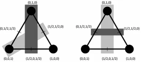
Consider for example the Hawk-Dove game discussed in the previous section. This is a two strategy game so our strategy space  is the unit line. We can plot the payoffs one receives from playing strategy 1 or 2 against the different strategy vectors as shown in Figure 3. This induces a convex division of into two best response regions ₁ and ₂. The update function

 

x

R



R F

is determined by considering how the points of

  

  





2 1,0 , 1 2,1 2 , 0,1

T (1.15)

are divided up into these best response regions. For example



1 2,1 2



R2 so F



 

1, 2



2.



For a 3 strategy game the simplex is the unit triangle. Again we can plot the payoffs one receives from playing pure strategies against strategy vectors in . In

Figure 4 (left) the x-y plane represents the different

strategy vectors, and the z coordinate representing the payoffs one receives from employing different pure stra- tegies against these vectors. Again this induces a division of the simplex  into convex best response regions.

Theorem 1 d k, 0

A partition of the points of d into subsets i d is induced by the best response division as-

sociated with some strategy game



if and

T mk

,  M

T W



[image:4.595.327.517.504.674.2]

k

[image:5.595.128.464.86.228.2]

Figure 4. On the left is an illustration of how pure strategies score different payoffs against mixed strategies in three strategy games. On the right is the best response division associated with the game described by Equation (1.6).

only if the convex hulls of each pair of distinct subsets and

i

W W_j do not intersect.

Theorem 1 allows us to determine when a given state regular automata is a best response game. The proof is in the appendix and the remainder of this section de- scribes the geometry of best response divisions in more detail. Given a non-singular payoff matrix we can find a division of the -dimensional space

k

M



k1



S into

(open) best response regions i. First we will consider

best response divisions of

R

S. Later we will consider

how such divisions divide up the points of the simplex of attainable strategies



: 0

  xS x



. (1.16)

For each pair i j, 



1, 2, , k



:i j let H

 

i j, S

be the set of all xS where

   

Mx_i  Mx _j. (1.17) The hyperplane is the set where the payoffs to pure strategies i and j are equal. Since M is non-

singular this hyperplane has dimension

 

i j,

H

2

k . The

hyperplane divides S into two regions, one where the

payoff to pure strategy exceeds that to pure strategy , and the other where the payoff to pure strategy

i

j j

exceeds that to pure strategy . Each of the i



1



2 n n

pairs

 

i j, define such a dividing hyperplane. The set



 

, 1,2, , : ,

i j k ijH i j





(1.18) of all of these hyperplanes together divide up the space

S into the distinct regions corresponding to the

distinct orderings of the payoffs at each point. The best response region i is the union of

!

k

k

R



k1 !



of

these regions, and these are necessarily contiguous. The set of regions correspond to the orderings of

, i.e. the permutations. The Cayley graph of the group k

!

k

,k





1,2,



S under the generator set of transposition of

adjacent elements corresponds to the adjacency of the

i. Each transposition corresponds to the crossing of a

hyperplane where there is equality of the payoffs for the elements which are transposed.

R

Alternately we can consider the sets

  

i  1, 2, ,k

  

 ,

B  i (1.19)

and H B



 

i



is the set of where the payoffs to

the elements of



x S

 

i

B are equal. Since is non-

singular there exists a unique value

M

1 T 1

 



 M l

x

l M l (1.20)

(A Nash equilibrium of the system.) Each H B



 

i



passes through x and on one side the payoff to is

greater than that to all the others, and on the other side it is less. We consider the set of rays consisting of

i

k

 

k

x and that part of H B



 

i





V

where the payoff to is less than the payoff to the other strategies, i. Since

our matrix is non-singular the set of rays form a basis for the simplex. For some set the convex combination of the corresponding rays, i V i is the

set where there is equality of the payoffs to the set of payoffs indexed by the elements not in , all elements in having lower payoffs. The regions i are the

interiors of the (closed) regions generated by convex combinations of points from . Each of these

closed regions is bounded by rays.

i

U



U

R



,k



V

 

i



1 1, 2,



V B



k

V

k

Thus we have that the division of the unit simplex into the best response regions is simply achieved by tak- ing a point in the hyperplane containing the unit simplex, and rays emanating from that point with the condi- tion that the reflection of any ray in the central point lies in the convex hull of the other rays.

k

k



k1



gions, and thus many payoff matrices. Suppose then that we are given the specification of the rays as a set of linearly independent vectors i for and

form the matrix which has the columns equal to the

i, then we select any matrix

u i1, 2, , k

U

u A with column

which have equal entries except for the diagonal entry which is smaller. Now we only require to find matrix

such that

ith

M



MU A (1.21)

i.e. , for this matrix M to provide us with

an appropriate payoff matrix, though we may require to add a constant to all elements if we require payoffs to be positive.

1

 

M AU

Example. Suppose the rays from the central equili- brium value are such that the matrix U is given by

1 2 3 3 2 3 4 1 3 1 2 4 4 4 1 2

 

 

 



 

 

 

U

Note that the columns add to a constant but this is not required. Now we can select any appropriate matrix A.

For ease we take , where is the unit matrix. We have

I I

0.5444 0.2333 0.3444 0.0111 0.3889 0.1667 0.3889 0.2778 0.1111 0.3333 0.1111 0.2222

0.3667 0.3000 0.0333 0.0333

  

    

  



 



M

   _    _

and we can add 1 if we require positive entries.

3. Games on the Circle with 2 or 3 Strategies

We can apply Theorem 1 to enumerate the two strategy best response games on the circle. To do this we must simply list all the different possible ways to divide up our simplex , the unit line, into two or less convex regions, with respect to the three points of —the lines two end points and the mid point.



2

T

There are only two ways of doing this, either all points belong to the same region or one end point belongs to one region and the other two points belong to the other. We can take each of these two unlabeled divisions and apply labels to the regions, deciding which best response regions they represent. We hence find that there are six non-identical two strategy best response game on the circle, three of which are permuationally distinct, mean- ing there are three fundamentally different types of two strategy best response games (see Table 1).

[image:6.595.77.266.393.449.2]

The first type are games where one strategy strictly dominates. These systems induce very dull dynamics with every vertex constantly playing the dominating strategy. Figure 1 depicts the dynamics of a game of the

Table 1. The payoff inequalities describe the three types of two strategy game that induce fundamentally different dy- namics in best response games on the circle.

Payoff inequalities that generate game type Example game

1,1 2,1

M M , M1,2M2,2 Trivial

2,1 1,1

M M , M2,1M2,2M1,1M1,2, M1,2M2,2 Hawk-Dove 1,1 2,1

M M , M2,1M2,2M1,1M1,2, M2,2M1,2 Stag Hunt

second type. The dynamics induced correspond to Wol- fram’s automata number 95. When the circle has even length there are two repelling fixed points, where no adjacent vertices share the same strategy. The system has many period two orbits which quickly attract other con- figurations. The third type of game corresponds to Wolf- ram’s automata number 160. When the circle has even length there is a repelling period two orbit—jumping between the two configurations with no adjacent vertices sharing the same strategy. The system has many fixed points which quickly attract other configurations.

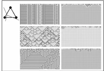
We can use Theorem 1 again to enumerate the best re- sponse games on the circle with three strategies. Recall how the best response division depicted at the right of

Figure 4 induces the dynamics depicted in Figure 2. Our theorem implies that any division of (which is the unit triangle) into three or less convex regions is induced by some game. The update function induced by such a division depends upon the way the six points of 2 (the 3 vertices and 3 edge-midpoints of the triangle) are par- titioned into these best response regions.



T

To enumerate all of the three strategy games we must simply list all the fundamentally different ways of divid- ing up  into three or less convex regions with respect to the points of ₂. There are 12 fundamentally different ways to perform such a division.

T

Each division induces an equivalence class, which is the set of best response divisions of ₂ which can be attained by taking and labeling the regions with dif- ferent strategies-deciding which best response region each region of represents. By looking at the different labellings of the 12 divisions we find that there are 285 non-identical three strategy best response games on the circle, 52 of which are permutationaly distinct. We give space time plots of the 52 cases in the appendix (sub- section 6.4), together with diagrams that show the di- visions corresponding to the equivalence classes of the games.

p

p

T

p

4. Games with More Strategies

Since the set of strategy best response games on the circle are a subset of the set of state regular automata one fruitful question to ask is when is a state regular automata on the circle not a strategy best response game?

k

D

k

k

k

G



2, We can think of each regular automata,

 



_{, ,} 0 _,

G S  G F

T





k S

, on a d regular graph , as inducing a partition of d in a similar way to the way we

did for best response games. To do this is that we think of our set of states as numbers and we think of each as a point

 

d

1, ,

S 

 

 

i D

 

d i



D d  



 e

P T (1.22)

in the simplex. We think of the points

 

 



: d

d  D D S

T P

mk

 

D

P

 



i

W

as being partitioned into subsets where W is the set of all points

such that F D i. i

The converse of Theorem 1 is that a regular automata is not a

k

strategy best response game if and only if the partition of



 

that

0

, , ,

G S  G F

 



_{, ,} 0 _,

G S  G F





d

induces has a distinct pair of sets and

T

i

W

j

W with intersecting convex hulls.

So to answer our question, we should find all of the pairs of disjoint subsets , d

 

X Y S such the convex

hulls of



P

 

D DX



and



 



intersect. We call such an D D Y

 P , X Y k S

 

1

pair ble be-

cause a state regular automata on a regular graph is not a best response game if and only if has a pair of states , such that



i



,

k d unaccepta



0

G S G

j

 

,F



, ,

d

 

, 1

F i F j are



k d,



unacceptable.

Clearly if a pair , d

 

X Y  S are such that there is

a pair X X and Y Y where X Y , are



m d,



unacceptable, for mk , then X Y, are un- acceptable. Knowing this we can tighten the definition of unacceptable pairs, to lessen the number of objects we need to catalogue to determine whether or not a regular automata is a best response game.



k d,



We say that a pair , d

 

X Y S



unacceptable if and only if  are fundamentally



k d, X Y, are



k d,



unacceptable and XX ,   , we

have that

Y Y  m k

,

X Y  are



m d,



unacceptable implies



X Y ,

 

 X,Y



and mk.

In other words a fundamentally unacceptable pair is an unacceptable pair that properly contains no other unac- ceptable pairs. So we arrive at Theorem 2.

Theorem 2 d k, 0

A state regular automata on a regular graph is a best response game if and only if , for every pair of states of , there does not exist a pair

k

k

 



G S, , G ,F



i j S

0  d m  

 

1

X F i , that is fun-

damentally

 

j

1

Y F



m d,



unacceptable.

Our enumeration problem is hence transformed into the problem of finding the set of permuationally distinct

fundamentally unacceptable pairs. The set of different convex partitions of d can be found by listing all the

permuationally distinct partitions of d and then filter-

ing out those partitions which involve a pairs

T

T

,

X Y such

that X X , Y Y

m k

is fundamentally unac-

ceptable, for





,

m d

 .

Let us consider the problem on the circle, when d 2. There are no fundamentally unacceptable pair

because



1, 2



 

 

2 ₁

 cannot be split into two disjoint non- empty sets. The fundamentally unacceptable pairs can be found visually, the only permuationally dis- tinct way one may choose two disjoint subsets



2, 2



A and

of

B ₂



  

  

0,1



such that the con-

vex hulls of 1,0 , 

T 1 2,1 2 ,

A and intersect is B A



   

1,0 , 0,1



and B





1 2,1 2 . The pair





X Y, , where

   



1,1 , 2, 2



X  and is hence the only

permuationally distinct fundamentally unaccept- able pair.

 



1, 2

Y 









2, 2

The set of fundamentally unacceptable pairs can again be found visually. It is easy to see that, if the convex hulls of two disjoint sets of T2, in the unit triangle, intersect, then one of the two situations depicted in Figure 5 must have occurred.



3, 2

For a pair of disjoint sets _, 2

 

X Y  S , let



,



Gr X Y be the graph with a vertex set consisting of

all xS such that x is a member of a pair in X or

, and edge set consisting of dark gray edges

Y X and

light gray edges Y . An alternating walk on such a graph



,



Gr X Y is a walk on the edges of such

that every edge traversed is a different colour to the previously traversed edge. An alternating cycle of such a graph is an alternating walk that finishes on the same vertex where it started returning along an edge of a dif- ferent colour to the colour of the edge that the walk first traversed.



,

Gr X Y



Lemma 1 A pair X Y, is



unacceptable if and

only if , 2



k



,



Gr X Y has an alternating cycle.

[image:7.595.310.539.570.671.2]

This leads to a result that allows us to completely cha-

Figure 5. The two fundamentally unacceptable pairs within the two dimensional simplex Δ. The left shows

 

3,2

   



2,2 , 1,3



,



   

3,3 , 1,2



, the right shows

   

racterise the et of fundam ntally s e

 

k, 2 unacceptable

n

C d

graphs for generic k. Recall that enotes the n vertex circle graph, let C1 be a single vertex with a self loop. Let a k vertex dumbbell graph Dum a b

 

, _k ,

where a b k , be the fusing of two c hs 1

a

C _ an to the two end points of a line graph (by

i entifying/ lapping vertices) so that the resulting graph, Dum a b

 

, _k , has k vertices (see Figure 6). Note that   b k 1, the connecting line be- tween the two circ

ircle grap d Cb

over1 when d

a es i

l n

 

a b, _k has no edges, and hence Dum a b

 

, _k resem ure-eight in that it consists of two circles intersecting at one vertex.

Let a good colouring of a graph G be a colouring of

its r

Dum

bles a fig

edges with dark gray and light ay such that, if a vertex vG only has two edges incident on it then the

two edg e painted different colours and otherwise two edges incident on a vertex v are painted different colours if and only if they do not lie on the same cycle of

G.

Theorem 3 ,

g es ar

X Y is fundamentally

 

k, 2 unaccept-

able if and only e of the following co ons hold: 1) k2 and

if on nditi



,



Gr X Y is a good colouring of

 

D 0,0 ₂

2k

um ;

is eve

2) n and Gr



X Y,



is a good colouring of

and is a good colou

C

 

,

k

Dum a b ,b



0,1, , k



are

even d such k;

3) 2k is odd Gr X Y



,



ring

of um a



k or

an

where a b

that a



, _k

D b where a b



,k



are even and

such k.

Using T 2 and lgorithm to ch

,  0,1, that ab

heorems 3 we can make an a

graphs, the different eck if a regular automata on the circle corresponds to a best response game and hence we can solve the problem of finding all of the fundamentally different 4 strategy best response games on the circle. The way we do this is to use a computer to generate the set of all four state de- gree 2 regular automata and then filter this set, removing those rules that do not correspond to best response games. We find that there are 143,524 non-identical four strategy games and 6041 permutationally distinct games.

5. Games on Other Graphs

When dealing with degree three

[image:8.595.61.285.645.690.2]

update functions F that can occur correspond to convex divisions of  with respect to the points of T3. With two strategies, we may enumerate the possible best re-

Figure 6. On the left is an illustration of Dum

 

2,0 . On ₅ the right is an illustration of Dum

 

5,0 . Both graphs have ₅

sponse games by listing the visions of the unit line

been given a good colouring.

different di

 into 2 convex regions with respect to the points of T₃



  

1, 0 , 1 3, 2 3 , 2 3,1 3 , 0,1

 

  



. Using this approach can determine the 5 permutationally

distinct update by two

strategy best response games on degree three graphs. Its important to note that the update rules found in this way could be evolved upon many different graph topologies. One could consider dynamics of the cube, the Peterson graph or any other degree three graph. The circle with self-linkage is the degree three graph obtained by taking a circle and linking each vertex to itself. Looking at best response games on the circle with self linkage is bene- ficial because the resulting one dimensional cellular auto- mata can be visualised using space time plots. The per- mutationally distinct two strategy best response games running on the circle with self linkage correspond to rules Wolfram’s elementary cellular automata numbers 0, 23, 127, 128 and 232. One may enumerate the different three strategy games on degree three graphs in a similar manner by listing the different ways to cut up the unit tri- angle into convex regions with respect to the points of

3

T . Using this method one finds that there are 82 fun-

damentally different three strategy best response games degree three graphs.

These methods can be applied to enumerate the num- ber of k strategy game

one

functions F that could be induced

on

s on degree graphs. Such an en

and

d

umeration seems difficult to do for generic k and d.

Theore 1 provides a way to do such an enumeration in theory but with no result like Theorem 3 (which allow us to quickly filter out unviable regular automata) the computation would be slow for d 2.

Our results can be extended to deal with non-regular graphs. Suppose we have a graph

m

s

G



di:1 i n



is the set of all di such that there is a

vertex of G with degree d_i. To numerat

nse games on G o e must simply list all

the differe ways to divide  into k or less convex

regions with respect to the points of ₁ i n

d iT



.

REFERENCE

e n

e the differ-

S

[1] J. von Neumann eory of Games and Economi University Press, ent best respo

nt

and O. Morgenstern, “Th c Behavior,” Princeton Princeton, 1944.

[2] J. Nash, “Non-Cooperative Games,” The Annals of Ma- thematics, Vol. 54, No. 2, 1951, pp. 286-295.

doi:10.2307/1969529

[3] J. Maynard Smith, “Evolution and the Theory of Games,” Cambridge University Press, Cambridge, 1982.

doi:10.1017/CBO9780511806292

[4] G. Szabo and J. Fath, “Evolutionary Games on Graphs,” Physics Reports, Vol. 446, No. 4, 2007, pp. 97-216. doi:10.1016/j.physrep.2007.04.004

ational Academy o Dynamics of Social Dilemas in Structured Heterogene Populations,” Proceedings of the N

ous f Sciences of the United States of America, Vol. 103, No. 9, 2006, pp. 3490-3494. doi:10.1073/pnas.0508201103 [6] M. Nowak and R. May, “Evolutionary Games and Spatial

Chaos,” Nature, Vol. 359, No. 6398, 1992, pp. 826-829. doi:10.1038/359826a0

[7] R. Southwell, J. Huang and B. Shou, “Modelling Fre- quency Allocation with Generalized Spatial Congestion Games,” IEEE ICCS, 2012.

r, Berlin, Heidelberg, 2012, pp. 31-46.

Some Models of Repro-[8] R. Southwell and J. Huang, “Convergence Dynamics of

Resource-Homogeneous Congestion Games,” GameNets, 2011.

[9] R. Southwell, Y. Chen, J. Huang and Q. Zhang, “Con- vergence Dynamics of Graphical Congestion Games,” Springe

[10] R. Southwell, X. Chen and J. Huang, “Quality of Service Satisfaction Games for Spectrum Sharing,” IEEE INFO- COM—Mini Conference, 2013.

[11] R. Southwell and C. Cannings, “Games on Graphs That Grow Deterministically,” GameNets, 2009, pp. 347-356. [12] R. Southwell and C. Cannings, “

ducing Graphs: I Pure Reproduction,” Applied Mathe- matics, Vol. 1, No. 3, 2010, pp. 137-145.

[13] R. Southwell and J. Huang, “Complex Networks from Simple Rewrite Systems,” arXiv Preprint arXiv:1205. 0596, 2012.

[14] R. Southwell and C. Cannings, “Exploring the Space of Substitution Systems,” Complex Systems, 2013.

[15] R. Southwell and C. Cannings, “Some Models of Repro- ducing Graphs: III Game Based Reproduction,” Applied Mathematics, Vol. 1, No. 5, 2010, pp. 335-343.

[16] R. Southwell and C. Cannings, “Some Models of Repro- ducing Graphs: Ii Age Capped Vertices,” Applied Ma- thematics, Vol. 1, No. 4, 2010, pp. 251-259.

[17] S. Berninghaus and U. Schwable, “Conventions, Local Interaction, and Automata Networks,” Evolutionary Eco- nomics, Vol. 6, No. 3, 1996, pp. 297-312.

[18] S. Berninghaus and U. Schwable, “Evolution, Interaction, and Nash Equilibria,” Journal of Economic Behavior and Organization, Vol. 29, No. 1, 1996, pp. 57-85.

doi:10.1016/0167-2681(95)00051-8

[19] C. Cannings, “The Majority Game on Regular and Ran- dom Networks,” GameNets, 2009, pp. 1-16.

[20] S. Wolfram, “A New Kind of Science,” Wolfram Media, 2002.

6. Appendix

6.1. Proof of Theorem 1

Any game



will induce a division of the ex- tended strategy space



,

G M

S into best response regions _i.

To show these best response region are convex, consider two points and within , then

R

x y R_i

   

Mx _i> Mx _j and

   

My_i  My _j,



1, 2, ,



j k

   i, by definition. Since is a linear

mapping any convex combination

M



1



x  y, for

 

0,1 







 



M x  y 

will be such that









 y



1 1

i  

  M x

j



i

,



1, 2, ,



j k

    . This means x 



1 



R

y also lies

within the best response region i. So every best res-

ponse region i is convex. This means our game in-

duces partition of d into best response regions

, such that the convex hulls of any two sets do not overlap.

R T

i i d

W R T



Wi Wj

Proving the converse is more involved.

Suppose we have a partition of the points of d into

sets Wi such that the convex hulls of each pair

of sets do not overlap. There will be a family of ap- propriate divisions of , into convex open sets , that generate such a partition of in that

T

mk

i

P

1

k

S k

T_d i,

.

i i d

Each such division, where every region i has non

zero volume, must be generated by a set of dividing hy- perplanes, which is a set of dimensional hyper- planes that cut up the space into different regions. Each

i is a polyhedral set and every dimensional

face of i is the intersection of the closure of i with

one of its neighboring regions. The set of dividing hyper- planes which generates such a division is the set of affine hulls of all such faces of all regions.



W R T

P

2 k

P k2

P P

Among our family of appropriate divisions there will be a division of S into non-zero volume, convex

sets i with the property that each set of

k

P k1 divid-

ing hyperplanes involved in this division will meet at a single point, we will call such a division proper. It is a well known result that almost every arrangement of

hyperplanes of dimension in 1

k k2 k1 will

have a common point, such a point will always exist provided no two of these hyperplanes have parallel sub- spaces. Any division can be made proper by doing an infinitesimal perturbation of the positioning of the divid- ing hyperplanes involved. Since the points of Td are

distantly spaced such a perturbation will not effect the way d is partitioned up. This means an appropriate

proper division exists.

T

Suppose i is a region within an appropriate proper

division. We shall use a proof by contradiction to show that i has a finite extreme point (a vertex). Suppose

(falsely) that does not have a finite extreme point.

P

P

i

P

Let X denote the closure of X . Any closed convex

set, like Pi, with no finite extreme point, must contain a

line L (extending infinitely in both directions). Any

translation of L that intersects with P_i must also be

contained within Pi. Let Pj be a region adjacent to i.

Any translation of

P L that intersects with _{i j} must

be contained within

P P

i j. This means any translation

of

PP

L that intersects P_j must be contained within P_j.

This argument can be continued to show that every re- gion contains a translation of L and every dividing

hyperplane contains a translation of L. This contradicts

our assumption that the division is proper because such an arrangement of dividing hyperplanes cannot meet at a point. Every k2 dimensional cross section of our hyperplane arrangement attained by slicing perpendicular to L will look the same (irrespective of how far along L one chooses to slice) so there cannot be a point where

all the dividing hyperplanes meet. This contradiction im- plies every region Pi must have a vertex.

1

Since Pi is k dimensional a vertex of i must

be the intersection of at least of its faces. Each of

i‘s faces is

P 1

k

P P_iP_j for some neighbouring region P_j.

There are only regions so k Pi can have at most

1

k faces. Hence _i has just one vertex , and is

the intersection of the closures of all k regions. Let

P v v

 

i

I be the intersection of the closures of every region

except i, it follows that will be a one dimen-

sional ray that is a common one dimensional edge of every region except i. There will be such one di-

mensional rays

P I

 

i

P k

 

i

I , that all meet at and every re-

gion

v

j

P will be the interior of the convex hull of

 







I a :a 1, 2, , k j



. Each ray must lie outside of

the convex hull of the other rays (otherwise the interior of two regions would intersect and we would not have a division). An equivalent way to say this is that the reflection of any ray in lies within the convex hull of the other

1

k

v 1

k rays.

Since our regions meet at a central point with emanating rays (that meet the appropriate conditions) we can use the results from section 0.2 to construct a non- singular payoff matrix which generates our convex division. Under the game with payoff matrix the th best response region will be equal to the convex region ,

k

M

i

R

M

i

i

P  i



1, 2,,k



. □

6.2. Proof of Lemma 1

We will show that a pairs unacceptability implies the presence of an alternating cycle. Suppose that

 

2 ,

X Y  S is a

 

k, 2 unacceptable pair, then by

definition, there must exist subsets X X, Y Y

and sets of positive reals



_{ a b,} 0 : ,

 

a b X



,

 

 

 ,  ,  ,   1

a b a b

a b X a b Y

 

 

 







,  (1.23)

and

   



   



   



   



, ,

, ,

2

2.

a b a b X

a b a b Y

a b

a b





 

 



 





e e

e e (1.24)

Now consider the graph with each dark gray edge weighted with the constant _{ }a b_,



,

Gr X Y 



 

a b, X 

and each light gray edge weighted with the constant _{ a b,}

 

,

a b Y

 . The sum of the weights of the dark gray edges incident upon any vertex will be equal to the sum of the weights of the light gray edges that are incident upon that vertex (where self edges are counted as being incident twice). Suppose is the minimal weight on any edge of , let us multiply all of the weights of ’s edges by

w







,

Gr X



,

Gr X Y



Y

 3 w, so that all of

the weights will be at least 3.

Now start on any vertex of , and walk along a dark gray edge, when the walk traverses an edge, reduce the weight of that edge by 1. After traversing a dark gray edge, let the walk traverse a light gray edge, then a dark gray edge, then a light gray... and continue in this manner, reducing the weight of every traversed edge. When an edge reaches weight



,

Gr X Y 

0



 it disappears and can no longer be used.

Every vertex must have at least two incident edges, one of each colour and such a walk is allowed to traverse each edge at least twice. Moreover, every time the walk approaches a vertex with an edge of one colour, it will be able to leave the vertex with an edge of the other colour (at least this will be true until an edge has been traversed twice). Clearly such a walk will be allowed to continue, in an alternating manner, until an edge is traversed three times. After an edge has been traversed three times it follows that some vertex must have been visited three times. This implies that an alternating cycle has been generated. To see this suppose, without loss of generality, that our walk first leaves along a dark gray edge. If the walk returns to , for the first time, along a light gray edge then an alternating cycle has clearly been generated. If, on the other hand, the walk returns to , for the first time along a dark gray edge then it must leave , for the second time, along a light gray edge. When the walk returns to for the second time it will complete an alternating cycle. To see this note that what- ever the colour of the edge which the walk uses to return to for the second time, the walk will have used an edge of the opposite colour to leave previously. This shows a pairs unacceptability implies the presence of an alternating cycle.

v

v

v v

v

v

v

v

To see the converse suppose that the graph Gr X Y



,



contains an alternating cycle Gr X Y



 ,



with X X, Y Y . Now 

 

a b, X let _{ a b,} be the number of

times that the edge

 

a b, is traversed in the alternating cycle Gr



X ,Y



. Similarly 

 

a b, Y let _{ a b,} be

the number of times that the edge

 

a b, is traversed in the alternating cycle Gr X



 ,Y



. We refer to _{ a b,} as

the weight of the dark gray edge

 

a b, X and we

refer to _{ a b,} as the weight of the light gray edge

 

a b, Y.

Our alternating cycle will be such that the number of traversals of dark gray edges must be equal to the num- ber of traversals of light gray edges, and hence our co- efficients will be such that

 a b, X  a b,  a b,

 a b, ,

Y

I

 

 

 

 





0

I

(1.25)

for some constant .

The alternating cycle will be a walk such that every time a vertex is approached along an edge of one colour the walk will leave the vertex along an edge of another colour and each edge

 

Gr

v ,

a b of is tra-

versed by this walk a number of times equal to its weight. It follows that, for every vertex of



,Y

X







,Y



X

Gr   , the

sum of the weights of ’s incident dark gray edges is equal to the sum of the weights of ’s incident light gray edges (where self edges are counted as being in- cident twice).

v

   

v

Hence we get

   





   



   



, ,

, ,

a b a b X

a b a b Y





 

 

2

2,

a b

a b



 





e e

e e (1.26)

so we can divide all of our parameters _{ a b,} and _{ a b,} by our constant I to get the set of convex coefficients

which describe a point where the convex hull of

 



P D DX



and



P

 

D DY



intersect. □

6.3. Proof of Theorem 3

Suppose X Y, is fundamentally unacceptable, then according to the definition of fundamentally un- acceptable pairs and lemma 1, is an alternat- ing cycle, and hence must be connected. Moreover there can only be one recolouring of the edges of



k



,

Gr X Y





, 2



X Y,



Gr ,

then is an alternating cycle (that recolouring which just swaps the colours of every edge). If this were not so then



,Y



Gr X would contain more than one fundamentally

different alternating cycle, and hence would not be fun- damentally unacceptable.