The Crude Oil Price Influence on the Brazilian Industrial Production

ISSN Online: 2329-3292 ISSN Print: 2329-3284

The Crude Oil Price Influence on the Brazilian

Industrial Production

Andre Assis de Salles, Pedro Henrique Acioli Almeida

Polytechnic School, Federal University of Rio de Janeiro, Rio de Janeiro, Brazil

Abstract

The oil price is a relevant variable for economic policy makers in countries where this commodity is the main energy source as well as in other countries where crude oil is not the only energy source. The sudden variations in the crude oil price cause direct influence in the national economies bringing changes in foreign trade, investments and productive activities. Therefore, the crude oil market is very important for the economic development. Further-more, crude oil is directly or indirectly present in all productive activities. This way the crude oil market is related to the industrial production indica-tors. Many researches aim at establishing the stochastic process that can represent the movements of macroeconomic indicators through the oil price returns or variations that have been done in recent years. The purpose of this work is to study the relationship between crude oil prices and selected indus-trial production indicators of the Brazilian economy. To do that this work carried out cointegration and causality tests, from VAR estimations, and im-pulse response analysis. The data used in this study is monthly macroeco-nomic indicators, mentioned above, and the Brent crude oil type price nego-tiated in the London Market. All data used is in US$. The period of the sample used is from January 2002 to October 2015.

Keywords

Oil Price, Industrial Production, Cointegration, Causality, Impulse Response Function

1. Introduction

Present in the global energy matrix crude oil is one of the most important energy sources in the world. It is an essential commodity in the global economy. Fur-thermore, petrochemical and chemistry industries produce or manufacture goods from petroleum, such as fertilizers used in agriculture for food industries.

How to cite this paper: de Salles, A.A. and Almeida, P.H.A. (2017) The Crude Oil Price Influence on the Brazilian Industrial Production. Open Journal of Business and Management, 5, 401-414.

https://doi.org/10.4236/ojbm.2017.52034 Received: March 23, 2017

Accepted: April 27, 2017 Published: April 30, 2017 Copyright © 2017 by authors and Scientific Research Publishing Inc. This work is licensed under the Creative Commons Attribution International License (CC BY 4.0).

Despite the progress in development of renewable energy sources in recent dec-ades, crude oil and their byproducts remain directly or indirectly present in people’s lives. Given this relevance, the crude oil price is an important variable for economic policy makers in national economies, where this commodity is the main source of energy as well as in worldwide economies.

The crude oil price movements are influenced by several factors that change randomly, for example, the weather, the available reserves, economic growth, changes in industrial production, political or geopolitical aspects, exchange rate variations, financial speculation, among others, such as sub-prime crisis and the recent fall in oil prices, caused by lower world demand or supply excess, events with large impacts on the crude oil market. These movements in crude oil inter-national markets directly influence the interinter-national financial markets and the economy in general, causing changes in foreign trade, investment and all pro-ductive activities. Even having many possibilities for renewable energy, crude oil has a significant participation in the Brazilian energy matrix. According to the Brazilian government oil and gas agency, in 2014 crude oil and natural gas to-gether accounted for approximately 44% of the Brazilian energy matrix. In countries with large reserves, the oil and gas industry often assumes an impor-tant role in economic development due to the high investments required for ex-ploration and production of reserves. In Brazil, it was not different, the oil is di-rectly or indidi-rectly present in all sectors, the movement of oil prices is consi-dered a relevant factor in the economic expectations.

Therefore many studies have been developed to verify the influence of oil price movements in economic activities, in economic performance and macroe-conomic indicators of national economies, such as gross domestic product rate, industrial production variations and changes of goods and services prices. These studies were conceived in order to establish a stochastic process, which represents the expectation of economic indicators activities of national econo-mies through oil price movements traded in the international market. Moreover, if the impact of oil price return in macroeconomic indicator is understood, it makes the verification of crude oil price impact possible. This allows firms to make predictions taking into consideration the impact on consumption as well as on the price level of their products. On the other hand, financial speculators may use the relation between oil price and macroeconomic indicators estimates to achieve extraordinary profits in the financial market while economic policy makers may use these very estimates to develop public policies that will allow for economic development and growth.

indi-cators and the oil price.

The remainder of this paper was structured as follows. The next section presents studies that deal with the impact of crude oil on macroeconomic indi-cators on different economies and periods. Section 3 shows the methodological approach description, divided into six distinct parts: stationarity tests, cointegra-tion tests, applicacointegra-tion autoregressive vector models (VAR) and vector models with error correction (VEC), causality tests and impulse response functions which is determined in the proposed econometric models. Section 4 presents the data used for this study is presented while the results obtained from the test and proposed models are presented in Section 5. The final comments are given in Section 6.

2. The Literature Review—A Brief

Given the importance of crude oil for economy, energy matrix and foreign trade, several studies has been done to observe crude oil price shock impacts on ma-croeconomic variables such as exchange rate, industrial production and trade balance, among others. These studies were carried out using various periods, countries or economic regions using different methodological approaches. Among these studies it must be highlighted the [1] work which, using monthly data between the years 1972 and 1993, searched for the relationships between the oil price and the US exchange rate. For crude oil prices, the West Texas Inter-mediate (WTI) type real price and deflated price was used, while for the ex-change rate, the real exex-change rate between the US dollar and fifteen currencies of developed countries was used. The reference [1] study stationarity tests for selected time series, which indicated that these series are integrated of order one, were performed. From the Johansen-Juseilus cointegration test, [1] presented evidence of cointegration between the two series, which show a long-term rela-tionship. Another inference highlighted by [1] is that the crude oil price causes the real exchange rate in the Granger sense, but the reciprocal is not true. The authors argue that the crude oil price has been dominated by shocks, especially in the 70s and early 90s, caused mainly by geopolitical conflicts and not by changes in demand from developed countries. Finally, [1] used a stochastic model with error correction mechanism, which showed significant predictive power for both values inside and outside the sample.

oil prices in economic activities in South Korea, Japan and Thailand, when a structural change in the 80s was considered. In other relevant inference, [2] hig-hlighted the existence of the oil price causality in the inflation of the six coun-tries surveyed. In a study that examines the relationship between the global eco-nomic activity, the exchange rate and the oil price, [3] used the Kilian index as parameter to measure the level of global activity and an exchange rate index be-tween the US dollar and a basket currency, as a proxy for the exchange rate. Us-ing monthly data, in the period from 1988 up to 2012, of crude oil price, the Ki-lian index and exchange rate cointegration test and Granger causality test were implemented, and pointed out that the oil price and global activity are cointe-grated.

The same occurs between oil prices and exchange rate. Therefore, it can be inferred that there is a long-term relationship between these variables. Another important inference by [3] pointed out that the economic activity index Kilian concerned to Granger oil prices in the international market influenced in the long term, the balance related to cointegration, as in the short term for the activ-ity world economic.

Another relevant study on this subject was conducted by [4] that infer the in-fluence of oil price impact in the international market and the exchange rate of the Russian ruble in the gross domestic product and tax revenues in Russia. The author used quarterly data for the period between 1995 and 2002, a period of major turbulence in the Russian economy, including the debt moratorium dec-laration in 1998. The reference [4] study used Phillips-Perron and Kwiatkowski Phillips-Schmidt-Shin (KPSS) tests to examine the time series stationary and concluded that time series studied did not have stationary in the level but can be considered integrated of order 1, or stationary at first difference. Reference [4]

conducted tests and estimated autoregressive vector models (VAR) concluding that both the exchange rate and the crude oil price, accounting for a half of its exports in 2004, has cointegration with GDP and tax revenue of the country. Reference [4] found evidence that, in the long-term, a 10% increase in oil prices is associated with a 2.2% increase in gross domestic product and 4.6% in tax col-lection in the country. While an appreciation in real terms the ruble was asso-ciated with a 2.7% fall in income, measured by gross domestic product. Despite the robustness of the statistical results, [4] points out that the parameter esti-mates should be viewed with reservations, since the analyzed period was short and extremely turbulent.

respec-tively, a decrease in industrial production by 19% and 18% in those countries.

3. Methodological Approach

Before using stochastic models for time series, it is important to check the viola-tion of basic assumpviola-tions. A common assumpviola-tion in many time series tech-niques of utmost importance is the stationarity. To test the stationarity of the time series worked in this study, the Dickey-Fuller test (ADF), inserted in the li-terature by [6], was used. When using non-stationary series, the estimation models of linear regressions, there is the risk of carrying out spurious regres-sions, that is, with apparent statistical significance of the coefficients of determi-nation but meaningless according to [7]. As noted by [8], considering Ztand Yt two non-stationary time series a linear combination of time series voids the sto-chastic trends making the new time series stationary which characterizes the two time series as cointegrated. The linear regression model can be estimated as fol-lows:

1 2 1 2

t t t t t t

Z =β +β X + ⇒ =e e Z −β −β X (1)

etis a stochastic term. If, by submitting this stochastic term to a unit root test to test its stationarity, it can be concluded that these two time series are cointe-grated and regression estimated between the two variables will not be spurious and, as highlighted by [9], there must be a long-term relationship between them. Reference [7] presents a detailed work about spurious regression when the va-riables related in regression models are nonstationary. Among the methods proposed in the econometric literature to test the cointegration in this research the Engle-Granger test, described in [10], was used to test the hypothesis of cointegration between the crude oil price and the selected macroeconomic indi-cators. This test simply consists of applying a unit root test, in this work the ADF test, to verify the stationarity of the stochastic term etor linear combination of the time series Zt and Yt. As the residual term is based directly on cointegrator parameter β2 and the critical values calculated by Dickey and Fuller are not ap-propriate, [10] have calculated critical values for the test (see [9]). The two time series cointegration refers to a long-term relationship between the series but nothing prevents imbalances in the short term. Therefore, as pointed out by [9], stochastic term et can be considered stationary as an equilibrium error and use it to relate the behavior of the two cointegrated time series in the short term with its equilibrium value long term.

In regression models, one variable is the dependent variable and the other the independent variable. However, there are situations where it is not exactly known which of the variables should be treated as a dependent variable. In these situations vector autoregressive models (VAR) can be used.

The VAR models are used to analyze the causal relationship between time se-ries. One can assume the following model in which Zt and Ytare stationary time series, that is, integrated of zero order or I (0):

1 2 1 3 1 1

t t t t

4 5 1 6 1 2

t t t t

Z =β +β Z₋ +βY₋ +ε (3)

In the equations described above, each variable depends on its value with a lag and another lagged variable. This equation system characterizes a vector autore-gressive model (VAR) and when using only one lag for each of the independent variables it becomes a VAR (1), or vector autoregressive model of order 1. The above can be used directly if the two time series Zt and Ytare stationary. Howev-er, if the time series are I (1) and are not cointegrated one should use the VAR with the first difference operators of these variables. Therefore, the equation sys-tem can be described as follows:

1 2 1 3 1 1

t t t t

Y β β Y− β Z− ε

∆ = + ∆ + ∆ + ₍₄₎

4 5 1 6 1 2

t t t t

Z β β Z− β Y− ε

∆ = + ∆ + ∆ + ₍₅₎

As all the above variables are stationary, one can estimate the model normally. In general, if the two time series are integrated of order n, one can use that number of differences in the model described above.

A large number of lags can be a problem for small samples, since the estimate of all parameters consume many freedom degrees of a VAR model. Furthermore it must be highlighted that if the variables are integrated of order 1 and therefore not stationary, but are cointegrated the equation system should be modified to take into account this long-term relationship. This modified version is known as vector model with error correction or VEC model. Thus, if two time series are integrated of order 1 and cointegrated they can be related in the following equa-tion:

1 2

t t t

Z =β +βY +µ (6)

By definition, since they are two cointegrated time series the stochastic term μt presents stationary behavior. The VEC model is used to estimate the system of equations below where all the terms are stationary, as in the VAR model below:

1 2 1 1

t t t

Y α α µ− ε

∆ = + + ₍₇₎

3 4 1 2

t t t

Z α α µ− ε

∆ = + + ₍₈₎

Using the values of residual term lagged µt−1, the VEC model can be repre-

sented as follows:

(

)

1 2 1 1 2 1 1

t t t t

Y α α Z− β βY− ε

∆ = + − − + (9)

(

)

3 4 1 1 2 1 2

t t t t

Z α α Z− β βY− ε

∆ = + − − + ₍₁₀₎

This system can be written in following form:

(

)

1 2 2 1 1 2 1 2 1 1

t t t t

Y =α − α β − Y− −α β +α Z− +ε (11)

(

)

3 4 1 1 4 1 4 2 1 2

t t t t

Z =α + α + Z− −α β α β− Y− +ε (12)

In the regression model above the parameters α2 and α4 are known as error correction coefficients, since they show the response magnitude of Zt and Yt va-riables given a variation of the residual term µt−1. To ensure stability, error

cor-rection mechanism coefficients must respect the following restrictions: α2∈

[

)

of the above restrictions, one can assume a situation in which the cointegrating regression shows a positive stochastic term in an accomplishment. These condi-tions guarantee that for a positive stochastic term, the ΔYt variation is positive and the ΔZt negative restoring the balance described by the cointegration. The lower modules of these parameters ensure that a system of equations does not present an explosive behavior.

Although the analysis of regression models describe the dependence of a va-riable in relation to the other, the existence of a regression does not necessarily imply a Granger causality. In time series analysis a recurring issue is the exis-tence and direction of causality between two variables. That is, the change in one variable causes a change in the other. To investigate the causality between the variables studied in this work we used the Granger causality test. One can as-sume two stationary time series Zt and Yt, for which there is interest in knowing if there is any causality between them. To do this, one can use the VAR with n

lags as shown in the equation system below.

1

1 1

n n

t i i t i j j t j t

Y =

∑

α

∑

β

ε

2

1 1

n n

t k k t k l l t l t

Z =

∑

γ

∑

δ

ε

The VAR model described above can be extended to more variables increasing the number of variables and equations in the model. This model relates the value of the variables with their lagged values and the lagged values of the other varia-ble. There are four possible scenarios. The first scenario would be one in which the estimated coefficients of the first lag Zt regression were jointly different from zero, and the estimated coefficients of the second lag Yt regression were jointly close to zero. In this case, there is a unidirectional causality from Yt to Zt. The Zt lagged values predict the variable Yt behavior, but lagged values of Yt do not contribute to predict the Zt behavior. In an unidirectional causality scenario in the reverse direction, there is the situation where the sum of the parameters βj is zero and the sum of the parameters γkis nonzero. A third possible scenario is the existence of bilateral causality: Yt causes Zt as well as Zt causes Yt. This scenario is characterized by the sum of parameters βj and the sum of the parameters γk that are both different from zero. Finally, when the above lagged values are all jointly equal to zero, that is, there is non-association between the variables Ytand

Zt. The null hypothesis of all the lagged coefficients being jointly equal to zero in the Granger causality test is tested by F statistics.

As noted by [11], the study of impulse response functions has the purpose of understanding the effects of random shocks in a time series. The impulse sponse function allows to verify the behavior of a variable when the other, re-lated to in the autoregressive vector model, suffers a shock or an impulse at a time t which propagates in future moments, for more details see [12]. A time se-ries described by the autoregressive model with a lag is shown below:

1

y

t t t

Y =ρY− +ν (15)

the values in this time series would behave given a unit shock at the start of the series, without other shocks. If ρ = 1, there is a unit root process and therefore the time series is no stationary. It should also be noted that in this specific case, the process would have infinite memory: the shock effect never scatters. Howev-er, when a value for the parameter is lower than a unit, the variable initially fully incorporates the shock value but returns to the null value, using the vector auto-regressive model (VAR) described above in the following form:

1 1

n n y

t i i t i j j t j t

Y =

∑

α

∑

β

ν

1 1

n n z

t k k t k l l t l t

Z =

∑

γ

∑

δ

ν

In the model above two possible shocks, one for each variable, are found. There are two response functions related to each shock, one for each variable. In total there are four response functions related to the VAR model and therefore it is possible to study the impact of a variable shock in the variable values itself and on the other variable values.

4. The Data—Sample Used

In addition to the crude oil price in the international market, the primary data used in this study refers to Brazilian industrial production indicators. The monthly crude oil prices used in this study were the Brent type crude oil prices traded in US dollars in London and collected from the EIA, the North American energy agency, for the period from January 2002 to October 2015. Indicators of industrial production, the industrial production indicators, released monthly by the Brazilian Statistical Institute (IBGE), were collected. According the IBGE these indicators are calculated by monitoring the production of about 830 prod-ucts in 3700 industrial places. The index is released according to the use of in-dustrial production categories, namely: 1) Overall Industry; 2) Consumer Goods; 3) Consumer Durable Goods; 4) Mining and Quarrying; 5) Manufacturing; 6) Capital Goods; 7) Intermediate Goods; 8) Semi and Non-durable Consumer Goods; and 9) Construction Inputs. The data used in this study were monthly industrial production indices by category of use, from January 2002 to October 2015, except for the construction inputs index, available only since January 2012.

To characterize the time series used in this study, statistical summaries were performed. These summaries are intended to observe the average, the disper-sion, the maximum, the minimum and the median values. Besides that the summary presents the skewness and kurtosis coefficients to verify the normality hypothesis, which is complementary with the Jarque-Bera (JB) normality hypo-thesis test. To characterize the time series selected, the stationarity hypohypo-thesis test, which is inserted in the summary, was performed.

1

Return ln t t

t

X X

X−

 

=  

  (18)

In the studied period, Brent crude oil price fluctuated between 19.4 and 132.7 US dollars per barrel, with average and median close to 70 US dollars. The price of Brent crude oil showed: asymmetry coefficient close to zero; a low coefficient of kurtosis, with a value of about 1.8; and a high volatility, measured by standard deviation of about 31.2 US dollars per barrel. The Brent oil price had higher values for their standard deviations when compared with their respective aver-ages. The skewness and kurtosis coefficients mentioned above show that these time series differ from a normal distribution time series, which is confirmed through the Jarque Bera test.

Table 1 above shows the industrial production indicators time series statistical summaries. As expected, the industrial production time series have averages and medians close to 100, the base value is 2012. As shown in Table 1, the industrial production of Capital Goods Index had the lowest average, with a value of 88.5, while the number of Construction Inputs Index showed the highest average, with a value of 96.2. The standard deviations of industrial production indicators present a wide range of values. The standard deviation of the industrial produc-tion of Capital Goods indicator, for example, is more than double of the Inter-mediate Goods and Construction Inputs indicators. The industrial production of Capital Goods has also the highest maximum, of about 127.1, while the industri-al production of Consumer Durable Goods has the lowest minimum, of about 48.5. The industrial production time series kurtosis and asymmetry coefficients that presented different values demonstrate varied behaviors from the

Table 1. Brazilian Industrial Production Indicators: 1) Overall Industry; 2) Consumer

Goods; 3) Consumer Durable Goods; 4) Mining and Quarrying; 5) Manufacturing; 6) Capital Goods; 7) Intermediate Goods; 8) Semi and Non-durable Consumer Goods; 9) Construction Inputs.

Industrial Production

Indicator (1) (2) (3) (4) (5) (6) (7) (8) (9) Mean 93.7 92.6 87.3 89.5 93.9 88.2 95.5 94.3 95.8 Median 93.8 93.4 89.8 91.6 93.4 88.5 95.9 94.3 96.2 Maximum 112.6 116.3 119.3 113.7 113.7 127.1 111.4 116.2 110.9 Minimum 69.7 67.4 48.5 58.9 70.4 50.4 74.8 70.5 81.1 Std Devition 10.0 11.4 17.8 13.3 10.1 20.5 8.2 10.2 8.5

Skewness −0.2 −0.2 −0.3 −0.4 −0.2 −0.1 −0.3 −0.1 −0.3 Kurtosis 2.3 2.4 2.2 2.0 2.3 1.9 2.5 2.4 1.9

JB test 4.96 3.54 7.76 9.99 4.51 9.12 3.99 2.53 2.46 p-value 0.08 0.17 0.02 0.01 0.11 0.01 0.14 0.28 0.29 ADF −2.13 −1.80 −1.82 −1.30 −2.11 −1.92 −2.69 −1.77 −2.72 p-value 0.23 0.38 0.37 0.63 0.24 0.32 0.08 0.39 0.08

normal distribution and the JB tests applied confirming it. The results of the JB normality tests indicate that the normality hypothesis should not be accepted for the Consumer Durable Goods, Mining and Quarrying and Capital Goods indus-trial production indicators time series. As can be seen in Table 2 ahead the monthly returns of Brazilian industrial production time series have low values of mean and medians, less than 1%. Noteworthy are the high modulus of the min-imum return of industrial production of Capital Goods, which reached −39%, and the maximum return of industrial production of Consumer Durable Goods, of about +35%. The industrial production of Consumer Durable Goods varia-tions also had the highest standard deviation, with a value of 12.5%. The kurtosis and asymmetry coefficients of the industrial production indicator variationsor returns showed very different values. Only Overall Industry, Mining and Qua-rrying and Intermediate Goods indicators showed positive skewness coefficients. The kurtosis coefficients showed values of around three, which is the value of a normal distribution. According to the JB tests, the null hypothesis of normality can not accept for the Consumer Durable Goods and Capital Goods series only.

As expected, the result of the augmented Dickey-Fuller stationarity test (ADF) for the Brent crude oil price time series point out for non-acceptance of the sta-tionarity hypothesis. The same applies to all nine series of industrial production indicators, that is, the hypothesis stationarity can not be accepted. For industrial production indicator variations, the results show no rejection of stationarity hy-pothesis for most of the series. Thus, considering the return series or variations of selected macroeconomic indicators, the stationarity hypothesis can not be ac-cepted only for the time series returns of Manufacturing, Capital Goods and

Table 2. Brazilian Industrial Production Indicator Variations: 1) Overall Industry; 2)

Consumer Goods; 3) Consumer Durable Goods; 4) Mining and Quarrying; 5) Manufac-turing; 6) Capital Goods; 7) Intermediate Goods; 8) Semi and Non-durable Consumer Goods; 9) Construction Inputs.

Industrial Production

Indicator (1) (2) (3) (4) (5) (6) (7) (8) (9) Mean 0.002 0.002 0.002 0.002 0.002 0.002 0.002 0.002 0.002 Median 0.000 0.008 0.011 0.001 0.002 0.005 −0.002 0.007 0.005 Maximum 0.166 0.180 0.350 0.159 0.170 0.233 0.148 0.160 0.126 Minimum −0.196 −0.188 −0.470 −0.138 −0.200 −0.317 −0.176 −0.163 −0.177 Std Devition 0.065 0.076 0.125 0.056 0.067 0.098 0.059 0.070 0.072

Skewness 0.077 −0.088 −0.379 0.055 −0.030 −0.390 0.254 −0.076 −0.424 Kurtosis 3.143 2.732 4.069 2.998 3.246 3.897 3.059 2.298 2.608

Semi and Non-durable Goods industrial production.

5. Results Obtained

As described earlier, the Engle-Granger test to examine the cointegration be-tween crude oil prices and industrial production indicator time series studied here was performed. In the Engle-Granger cointegration tests, two regressions were performed for each industrial production indicators and crude oil price time series. In the first regression variable one variable is dependent and the other is independent, in the second regression the dependence changes. The cointegration hypothesis is not rejected only if both regression models indicate that cointegration hypothesis should not be rejected. If they are not, one should reject the null hypothesis and conclude that the series are cointegrated and therefore, there is a long-term relationship between them.

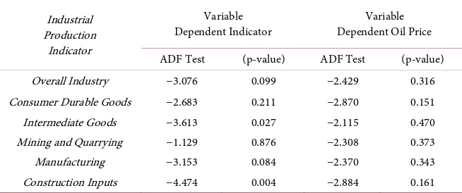
Table 3 shows the cointegration test results. It is possible to infer, at the 10% level of significance, that the Brent crude oil price is cointegrated with the Over-all Industry, Intermediate Goods, Manufacturing and Construction Inputs in-dustrial production indicators. It must be highlighted that the inin-dustrial produc-tion of capital goods and semi-durable and nondurable goods are integrated in more than one order, that is, nonstationary for difference. It would be inappro-priate to use them in Engle-Granger cointegration tests. For those time series that showed no cointegration the VAR models are used to observe the behavior of time series returns studied here and the significance of crude oil price on them. These models were built using the log returns or the log variations of the time series studied. As shown in Table 1 the macroeconomic indicator time se-ries do not present stationarity. This occurs also with the crude oil price. The lag numbers for all VAR model estimated were determined using the Akaike criteria selection model limited up to 12 lags or 12 months. The values of Akaike criteria for various lags can be observed in Table 1, in which the lag numbers for each model are indicated.

The Granger causality test is determined through these bivariate VAR models estimated with the Brent crude oil price returns and industrial production indi-cators selected for this work, that is, these tests verify if the returns after Brent

Table 3. Cointegration test results.

Industrial Production

Indicator

Variable

crude oil price used in the model cause the contemporary variations of the va-riables studied. As described earlier the Granger causality hypothesis test con-sists in verifying if the coefficients of the VAR model are jointly close to zero. It can be inferred that the Brent crude oil price returns, at a 10% level of signific-ance, cause the industrial production time series variations for durable consum-er goods, intconsum-ermediate and mining industry goods. Thconsum-erefore, it is possible to infer that at a 10% level of significance that the Brent crude oil price returns should explain the Brazilian industrial production indicators studied.

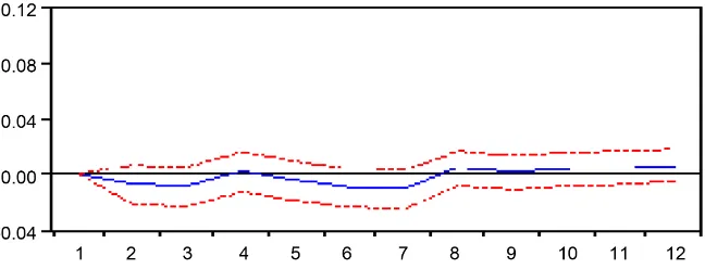
To obtain impulse response functions that permit to observe the oil price re-turn shocks repercussion in the Brazilian industrial production indicators, VAR models were proposed. As mentioned in the methodological approach each VAR model estimated has four impulse response functions associated, that are pre-sented from Figures 1-3 shown below. The solid lines show the dependent vari-able expected behavior before a shock while the dashed red lines show the error average of response expectations interval.

In Figure 1 the VAR model impulse response function of Brent oil price re-turn and the industrial production index for durable consumer goods variations are shown. This index respond quickly to a shock of about 8% in crude oil prices returns with a 1.5% positive variation but it was dissipated in around 3 months’ time. Figure 2 and Figure 3 present the VAR model impulse response function for Mining and Quarrying industrial production and Intermediate Goods indus-trial production indices variations.

Figure 1. IRF-oil return to consumer durable goods industrial production indicator

vari-ation.

Figure 2. IRF-oil return to mining and quarrying industrial production indicator

Figure 3. IRF-oil return to intermediate goods industrial production indicator variation.

Both have little relevance responses to shocks in the oil price returns. The Mining and Quarrying industrial production index show a response of 0.05% to a crude oil price returns impact with lagged about three months, to a crude oil price return shock of around 8%, in which the Brent oil price return was quickly dissipated. The Brent oil price returns has no significant response to shocks on the Mining and Quarrying industrial production index variations while each in-termediate goods production index variations have an response about 1% to 8% shock in oil prices return, and also this response quickly was dissipated.

6. Conclusion and Final Comments

This study aimed to test hypothesis for establishing short and long-term rela-tionships between industrial production indicators of the Brazilian economy and crude oil price in the international market.

It must be noted that industrial production indicators of the Brazilian econo-my time series stationary test conducted indicated that the industrial production of Capital Goods, Consumer Goods as well as Semi and Non-durable Consumer Goods time series are integrated in an order greater than unity. Thus, the stationa- rity assumption can not be accepted for these time series, hindering the work done here. Another problem to be observed concerns the period studied. In the sample interval, fuel prices in Brazil did not fluctuate freely once the Brazilian government authorities imposed a fuel price control seeking to contain inflatio-nary pressures, that is, in an attempt to control prices in the economy. Through the cointegration tests, it can be inferred that there is evidence of a long-term relationship between Brent crude oil price and indices of Overall Industry, In-termediate Goods, Manufacturing and Construction Inputs. The causality tests point out that the Brent oil price returns should allow the understanding of in-dustrial production sectors variations in the Brazilian economy, namely: the Consumer Durable Goods, the Intermediate Goods and the Mining and Qua-rrying industry. Finally, the impulse response functions from the proposed au-toregressive vector models were obtained.

Thus, the preparation of studies seeking to establish appropriate models for the prediction of the Brazilian economy leading indicators, which can provide al-ternatives to formulate key economic policies for the Brazilian economic growth, is what is suggested for future works that may continue this research.

References

[1] Amano, R.A. and van Norden, S. (1998) Oil Prices and the Rise and Fall of the US Real Exchange Rate. Journal of International Money and Finance, 17, 299-316. [2] Cuñado, J. and Gracia, F. (2005) Oil Prices, Economic Activity and Inflation:

Evi-dence for Some Asian Countries. The Quarterly Review of Economics and Finance, 45, 65-83.

[3] Yanan, H., Wang, S. and Lai, K.K. (2010) Global Economic Activity and Crude Oil Prices: A Cointegration Analysis. Energy Economics, 32, 868-876.

[4] Rautava, J. (2014) The Role of Oil Prices and the Real Exchange Rate in Russia’s Economy: A Cointegration Approach. Journal of Comparative Economics, 32, 315- 327.

[5] Bayar, Y. and Kilic, C. (2014) Effects of Oil and Natural Gas Prices on Industrial Production in the Eurozone Member Countries. International Journal of Energy Economics and Policy, 4, 238-247.

[6] Dickey, A.D. and Fuller, A.W. (1979) Distribution of the Estimators for Autoregres-sive Time Series with a Unit Root. Journal of the American Statistical Association, 74, 427-431.

[7] Granger, C. and Newbold, P. (1976) R² and the Transformation of Regression Va-riables. Journal of Econometrics, 4, 205-210.

[8] Cochrane, J.H. (1997) Time Series for Macroeconomics and Finance. University of Chicago, Chicago.

http://www.bseu.by/russian/faculty5/stat/docs/4/Cochran,TimeSeries.pdf

[9] Gujarati, D. (2004) Basic Econometrics. 4th Edition, McGraw-Hill Companies, New York.

[10] Engle, R.F. and Granger, C.W. (1987) Co-Integration and Error Correction: Repre-sentation, Estimation and Testing. Econometrica, 55, 251-276.

https://doi.org/10.2307/1913236

[11] Hill, C. Rand Griffiths, E.W. (2008) Principles of Econometrics. 4th Edition, John Wiley & Sons, New York.

[12] Enders, W. (2009) Applied Econometric Time Series. 3th Edition, John Wiley & Sons, New York.

Submit or recommend next manuscript to SCIRP and we will provide best service for you:

Accepting pre-submission inquiries through Email, Facebook, LinkedIn, Twitter, etc. A wide selection of journals (inclusive of 9 subjects, more than 200 journals)

Providing 24-hour high-quality service User-friendly online submission system Fair and swift peer-review system

Efficient typesetting and proofreading procedure

Display of the result of downloads and visits, as well as the number of cited articles Maximum dissemination of your research work

Submit your manuscript at: http://papersubmission.scirp.org/