On the Eonomic Purpose of General Purpose Technologies: A Combined Classical and Evolutionary Framework

Munich Personal RePEc Archive

On the Eonomic Purpose of General

Purpose Technologies: A Combined

Classical and Evolutionary Framework

Strohmaier, Rita and Rainer, Andreas

Department of Economics, University of Graz, Graz Schumpeter

Centre, University of Graz

5 April 2013

On the Eonomic Purpose of General Purpose

Technologies: A Combined Classical and

Evolutionary Framework

Strohmaier R.

_{, Rainer A.}

April 5, 2013

Abstract

General purpose technologies (GPTs) are technical breakthroughs that are able to spur growth via their pervasive use in the economy. This paper at-tempts to study the effects of these innovations for the economic system on an empirical and theoretical level. A structural decomposition analysis for Denmark from 1966 to 2007 tracks the impact of the current GPT, the in-formation and communication technology (ICT), on aggregate and sectoral labor productivity growth. Findings show that the broad diffusion of ICT affected growth significantly after 2000, owing to technical change, substi-tution and capital deepening, and can be associated with skill-induced wage dispersion. The diffusion process of a GPT is subsequently reconstructed by an evolutionary multisectoral framework: The Sraffian input-output ap-proach is combined with the replicator dynamics apap-proach of evolutionary game theory. Technical unemployment, transitional wage inequality and de-celerating economic growth after the appearance of a GPT can thereby be explained.

∗_{University of Graz, Department of Economics, Universitaetsstrasse 15/F4, A-8010 Austria:}

[email protected].

1

Introduction

By 1900, 38 per cent of vehicles in the U.S. were electric; 40 percent were steam powered and only 22 percent used gasoline. However, because of the limited driving range of electric vehicles and the lacking infrastructure for recharging, the technical advances in internal combustion engineering literally drove the rise of gas-powered automobiles. In 2004, automobiles and light trucks in the USA were responsible for nearly half of all greenhouse gases emitted by automobiles globally, according to a recent study by DeCicco and Fung (2006). Back in 1900, if innovative activities would have been channeled to the prevailing technology, the economy and the environment would have developed along a different, probably more sustainable, path. So history matters and some innovations are able to make history.

This is particularly the case of general purpose technologies (GPTs): major technological breakthroughs that shift physical restrictions and spur growth via their pervasive use in the economy. Prominent examples are the steam engine and electricity, and lately the new information and communication technology (ICT). To understand the inter-sectoral spill-over effects by the emergence of a GPT re-spectively by technical change within a GPT-producing sector therefore facilitates the understanding of economic and social consequences of technical progress. For instance, the productivity slowdown of advanced economies (especially of the U.S.) experienced in the 1980s, followed by substantial growth in the following decade, can be linked to some extent to the rise of ICT: Basic arguments for the slump brought about by ICT were the irreversibility of tailor-fit inputs, obsolescence of capital and a short supply of skilled labor (Helpman,1998).

2000s. Inklaar and Timmer (2007) compared seven economies1 _{with regard to}

industry output, input and multi-factor productivity (MFP) levels. They showed that the U.S. used twice as much ICT-capital than Anglo-Saxon countries where production tends to be more labor-intensive. This high level of IT-capital can be found across all sectors of the American economy. In a recent article, Jorgenson

and Timmer (2011) show that the rapid productivity growth (in terms of MFP)

in the European Union, the U.S. and Japan is accompanied by the growing role of service sectors, the decline of the labor share in value-added, and the increased use of IT-capital across all regions and sectors.

Even though the ICT revolution, starting in the U.S. in the 1960s, took several decades to show up in productivity growth in the computer-using industries, the wage of skilled workers has risen significantly from the emergence of this GPT onward. The most common explanation is that the efficient utilization of ICT makes great demands on the qualification of the workforce: New skills are required that first need to be obtained through investments in education and on-the-job-training. Thus, increasing computerization has been associated with higher levels of both skills and wages in the workforce (Majumdar,2008; Allen, 2001;D. Autor

and Krueger, 1998; E. Berman and Griliches, 1994; Krueger, 1993), as well as

with the substitution of low-skilled by higher-skilled workers (Levy and Murnane,

1996). Thus, the rapid skill-biased technical change has resulted in rising wage inequality both among and within different education groups, despite an increasing supply of better qualified labor (see e.g. Murphy and Welch (1992); D. Autor

and Krueger (1998)). The relation between the emergence of a GPT and skill

and wage differentials have been extensively discussed in the theoretical literature (see e.g. Helpman and Trajtenberg (1998b,a) and Nahuis (2004) for a general equilibrium approach). Furthermore, Aghion and Howitt (1998a, 2002) propose a Schumpeterian framework for explaining the evolution of wage inequality.

This paper aims at contributing both to the empirical as well as to the theoret-ical literature. It therefore advances along two dimensions: (1) On the empirtheoret-ical level, the paper attempts to assess the impact of ICT (the current GPT) on

ag-1

gregate and sectoral productivity for Denmark between 1966 and 2007 by use of a structural decomposition analysis (SDA). Denmark is chosen due to the extent of the available data and its size, which characterizes it as a small open economy. We revert to labor productivity growth, since ICT has had a special impact on the labor market: On the one hand, labor intensity of production decreased through automation owing to ICT-capital, on the other hand the IT-boom has raised the demand for qualified workers. Combining the Sraffian (price-) with the Leontief (quantity-) system, annual changes in labor productivity are decomposed into dis-embodied technical change, shifts in the employment of low and high skilled labor, factor substitution, and technical change embodied in capital goods. Contrast-ing these results with the changes in the electricity sector allows comparContrast-ing the different maturity stages of these general purpose technologies. (2) Supported by empirical evidence, the theoretical part of the article proposes a Sraffian multi-sectoral approach that is embedded in an evolutionary framework. This model is capable of reconstructing the output slump after introduction of a GPT as well as transitional wage inequality during the diffusion process of the new GPT.

The paper proceeds as follows: Section 2 introduces the inter-sectoral frame-work. Section3describes the structural decomposition analysis and the underlying data. A detailed presentation of the SDA and the industry classification can be found in the Appendix. Section 4displays the most important results with a spe-cial emphasis on the GPT at work, ICT. In Section5the Sraffian static framework is augmented by the replicator dynamics approach of evolutionary game theory to gain some deeper understanding of how the inter-sectoral linkages work. Conclud-ing remarks are given in Section 6.

2

Methodology and notation

the economic implications of some GPT in a multi-sector setting. Therefore a classical input-output model developed by Piero Sraffa (1960) serves as the ba-sis of our investigation. Subsection 2.1 introduces the general notation for the long-period position of the economy. This prepares ground for two further steps: Firstly, for the structural decomposition analysis outlined in Subsections 2.2 and in the Appendix A.1 for further refinement of the subsequent empirical analysis; and secondly for embedding the static model into an evolutionary framework in Section5 to investigate dynamical aspects of the diffusion process.

2.1

A Sraffian multi-sectoral framework

In an N-sector economy, let amn ∈ (0,1) be the amount of good m produced in

sectormto produce one unit of output in sectorn. A new GPT such as the ICT is accompanied by new skills necessary to operate the innovative technologies. Skill diversification, including the existence of wage premia, is considered by allowing for K different skills. lmk > 0 then denotes the quantity of skill k necessary to

produce one unit of output of sector m. The input matrices A ∈ [0,1]N×N

and

L∈RN×_K

+ with coefficientsamn and lmk characterize the utilized technology. The

n-th entrypnof the price vectorp ∈RN+ denotes the price of commodityn. wis the

wage vector with thek-th entrywkdenoting the remuneration of skillk. Assuming

prices to be determined by unit costs of production, one gets the following price system

(1 +r)Ap+Lw=p (1) with normal rate of profitsr(Kurz and Salvadori,1995). Defining some commodity bundle d ∈ RN+ as num´eraire by dTp = 1 and wage level w = kwk, the falling

w−r relationship

w= 1

dT _{(I−(1 +r)A)}−1

Lu (2)

0 0.2 0.4 0.6 0.8 1 1.2 1.4 0

0.5 1 1.5 2 2.5 3 3.5x 10

−4

1966 1976 1986 1996 2006

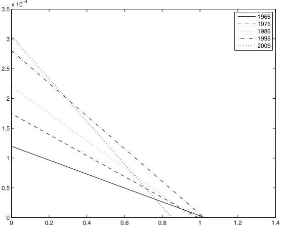
Figure 1: Wage-profit curve for Denmark from 1966 to 2006

corresponds to an anti-clockwise rotation. Hicks-neutral or factor-saving techni-cal change leads to a parallel shift outwards. If two curves–related to different technologies–intersect, then technical progress is not unambiguous and one has to draw on actual income distribution w and r to scrutinize the sort of change

(Degasperi and Fredholm,2010, p.274).

Figure 1 shows the corresponding wage-profit-frontier for Denmark from 1966 to 2006. The intersection with the axes determines the maximum wage rate (for

r = 0), and the maximum rate of profits (for w= 0) respectively. Until 1986 the curve rotates clockwise around a more or less stable rate of profit in the range of 0.92. Since this value is in reality unlikely to occur, one can conclude that in the 20 years between 1966 and 1986, labor-saving technological change took place. For 1996 the w−r-relationship shows unambiguous technical progress, because both intersection points moved outwards. Since then, however, the maximum rate of profits has decreased and the curves of 1996 and 2006 intersect at a rate of profit equal to 0.31. Comparing this value to the average interest rates for 20062 _{it is}

2

clear that within a realistic range of profit rates the latter technique turns out to be labor-saving and capital-using relatively to the former production system.

In the case of a zero profit rate r = 0, equation (2) reads

¯

w= 1

dT _{S Lu} (3)

with the Sraffa Inverse S ≡ (I−A)−1

. The higher ¯w, the less direct and indirect labor inputs are necessary for the production of the exogenously specified com-modity bundle. An increase in the maximum wage rate over time thus indicates productivity gains due to technical progress. The relative change in the maximum wage rate from one year to the next therefore provides a measure for the annual labor productivity growth:

gl t =

¯

wt−w¯t−1

¯

wt−1

= ¯wt

1 ¯

wt−1

− 1

¯

wt

(4)

This measure differs from the conventional indicator of labor productivity growth in so far as it considers not only the labor that is directly employed in the respective sector, but also takes into account the labor input in the upstream production. This means that an industry exhibits a higher labor productivity (as defined by Eq.3) whenever the supplying industries operate less labor-intensively.

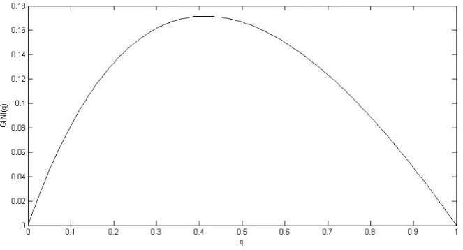
Labor productivity growth is in case of innovations accompanied by the emer-gence of new skills and respective skill premia captured by the vector u in equa-tions (2) and (3). For the simple case of two different skills, and each employed in another process within the economy, wage inequality can be calculated by

GIN I =qh(1−qh)

u−1 1 + (u−1)qh

, (5)

whereqh denotes the share of high skilled labor which is utilized by the innovative

process and remunerated by some wage premium u >1 relative to the low skilled labor utilized by the incumbent technology. Figure 2 graphically demonstrates the dependence of wage inequality on the share of high skilled labor with a wage

Figure 2: The GINI coefficient depending on the share of high-skilled labor

premium of u= 2.

2.2

Structural decomposition analysis

SDA has been a prominent tool in input-output analysis for associating changes in one variable, most often gross output or value-added, to changes in other variables (Miller and Blair,2009;Rose and Casler,1996;Dietzenbacher and Los,1997,1998). With regard to labor productivity, Yang and Lahr (2008) use two multi-regional input-output tables of China to decompose the change in labor productivity growth between 1987 and 1997 into five determinants3 _{and subsequently assess the results}

at a regional level. In a follow-up study, the analysis is extended to further com-ponents, with a special focus on the intra- and inter-sectoral composition of final demand, and extended to the year 2005 (Yang and Lahr, 2010). The account-ing framework goes back to Jacob (2003), who analyzed the growth experience in Indonesia between 1971 and 1995, distinguishing between a pre- and a post liberalization phase.

In this paper, SDA is used to break down the change in the maximum wage rate

3

(labor productivity) into its different components. Therefore the afore discussed Sraffian model is coupled with the analytical framework developed by Wassily Leontief4_.

In the Leontief system, gross output x is calculated from the demand side, as market clearing implies

xTA+yT =xT.

y gives total final demand (from private households and government, investment and exports). Furthermore, total labor demand l(weighted by its relative wages) can be calculated as the product of the labor intensity L and the gross output vector x:

l= diag(Lu)x= diag(Lu)Hy (6)

H ≡(I−AT₎−1

=ST _{denotes the Leontief Inverse.}

Combining (6) with (3), the maximum wage rate is given by

¯

w= 1

dT _{S Lu} =

1 dT _Sˆl ˆx−₁

e =

1

dT _Sˆl_[diag(Hy)]−₁

e, (7) where ˆ indicates a diagonalized vector and e ∈ RN _{is a vector with coefficients}

en = 1 for alln = 1, . . . , N. Considering two different snap shots in time, from (4)

and (7) labor productivity growthgl

t can be derived as

gl

t = wt dT

h

St−1ˆl_t−1 [diag(H_t−1y_t−1)] −1

−Stˆlt diag(Htyt)]

−1

)ie. (8)

Given equation (8), the relative change in the maximum wage rate can be decomposed into four partial factors: (1) technical change as indicated by a change in the direct input matrix A (∆S ≡St−St−1), (2) change ∆l≡l_t−l_t−₁ of total

employment, (3) substitution effect indicated by a change inAT _{(∆H ≡Ht−H} t−1)

and (4) change ∆y ≡ yt −yt−1 of final demand. This initial decomposition is

extended by differentiating between low and high skilled labor, and capital flows

4

of ICT and Non-ICT related investments. The decomposition can be found in detail in A.1.

3

Data

3.1

National account data

Denmark is used as a case study for the following two reasons: Firstly, it is a small open economy acting as a net-importer of ICT-products5_{. ICT can therefore be}

analyzed from a more general perspective, since the focus is on the impact of a GPT as an input of production and not on its impact on final demand. Economies such as the U.S., Japan or Finland – which are net-exporters of ICT-products – would cause a bias with regard to this research question: It is their extensive trade with these products that affects economic development, and not primarily the pervasive use of this GPT in production.

Moreover, Statistics Denmark also provides a very good data base that fits the purpose of this work: Annual IO tables for 130 sectors in ISIC 3.2. Rev. classi-fication, in current as well as constant prices of the year 2000, entailing domestic and import flows, and covering a long period of time (1966 to 2007). Applying the criterion of Jovanovic and Rousseau (2005a), whereby the emergence of a GPT can be dated to the year when the new technology reaches a one percent share in the industrial sector’s stock equipment – which in Denmark’s case was in 1979 – we can therefore also study the pre-arrival time.

The 130 sectors in the original classification were subsumed under 53 indus-tries for the sake of better illustration of the results and in order to ensure the non-singularity of the system (see Table2inA.2). In the following, the years 1970 until 1972 will be excluded due to the lack of data reliability, because for these periods the results indicate a hardly viable system (i.e. with a profit-rate close to zero). Concerning the definition of the ICT-producing sector, a broad classifi-cation scheme is used, including not only the ICT manufacturing sector, but also

5

computer related business activities and software consultancy. The following in-dustrial and service classes comprise the notion of ICT in the scope of the present analysis: (1) Mfr. of information and communication technology (ICM): Mfr. of office machinery and computers, Mfr. of other electrical machinery and apparatus, Mfr. of radio and communications equipment etc. (2) ICT-related services (ICS): Computer activities, Software consultancy and supply.6

Investments in ICT capital deserve a special consideration, since most ICT products are not used up within one period, but remain in the production process. Thus the analysis needs to include investment flows as well. From 1993 to 2007 real investment matrices, in constant prices of year 2000, were available in 5 categories: (1) buildings other than residential, (2) machinery, (3) transport, (4) software, (5) construction. The classification of delivering sectors is identical to the one in the IO-scheme. However, the set of investing sectors corresponded to the national standard classification of 53 sectors, whereby 3 industries (health, research and education, culture) are further disaggregated, resulting in 56 sectors in total. In a first step, the investment matrices were re-classified according to the 53 sectors in the Sraffian classification, which was in most cases a one-to-one concordance. The only industry that needed to be split up further was electricity, since in the original classification it is presented together with gas and water supply. The assigned share was therefore derived from total deliveries of these two sectors to investment demand. However, the distribution across sectors was assumed to be the same for the electricity and the gas and water supply industry. Investment demand before 1993 was only available at an aggregate level in the aforementioned categories (1)– (5). For these years, the sectoral shares in the demand for the respective asset were calculated from the purchases of intermediate products. It is therefore assumed that sectors with higher demand for intermediate (circular) products also invest more in this technology. These estimations were backed up with investment data (industry by industry) from 1966 to 1992.

6

3.2

Employment data

As regards employment, total working hours of employed persons and self-employees were obtained from Statistics Denmark. For the discrimination of the labor force according to the attained education we used the Denmark labor input data pro-vided by the EU KLEMS database (Edition 2008). This dataset comprises the shares in total hours worked as well as the shares in total labor compensation for three different qualification levels for a time-span of 26 years (1980–2005). Since these data are only broken down for 15 sectors, each subsector is approximately characterized by the same labor composition. For the purpose of this paper, only between low-skilled and higher (i.e. middle and high)-skilled workers was discrim-inated; no differences in age and gender are considered. For Denmark, low-skilled labor refers to basic schooling, whereas middle and high skilled labor comprises short, middle and long cycle higher education as well as vocational education and training (for further details on the labor accounts see the EU KLEMS manual, pp. 24–31). For both qualification levels, the ratio between the respective wage share and the share in total working hours is calculated in order to obtain the compensation level of the respective skills compared to the industry average.

3.3

A note on the num´

eraire

1966 1971 1976 1981 1986 1991 1996 2001 2006 2011 −0.05

−0.03 −0.01 0.01 0.03 0.05 0.07

0.09 LPG national accountsLPG SRAFFA

Figure 3: Growth of labor productivity (LPG) from 1966 to 2007. Figures from the Sraffian system and the system of national accounts.

the monetary IO-tables are set out in constant prices as of 2000.7

dn =

xn−

P53

j=1znj

P53

n=1

P53

j=1ynj

Figure 3 presents the growth of labor productivity (LPG) obtained from the national accounts,8 _{together with the productivity measure derived from the}

Sraf-fian system (solid line). The LPG measure deviates in two years (1981 and 1983) from the indicator based on national accounts, but otherwise represents a good fit to the conventional figures (with a correlation-coefficient ρ= 0.87).

7

Since competitive imports are included in the transaction matrix, a negative net output is likely to occur in those periods where domestic production depends largely on imported interme-diate products. Therefore it is necessary to ensure that the num´eraire is strictly positive. Note that the more negative the net-product, the higher would be the positive impact of the sector on the productivity measure, thus causing a severe bias on the aggregate level.

8

4

Results and Discussion

The results of the SDA are presented first on the aggregate level (Subsection 4.1) and then with regard to the ICT (Subsection 4.2). In the latter part a discussion is included how the diffusion of ICT is linked to the evolution of wages and wage inequality.

4.1

Aggregate results

Figure 3 shows that labor productivity growth has been steadily decreasing in the past 40 years: 4.0% per annum in the 1960s compared to around 1% in the last decade. These historically low growth rates also lag behind other countries: Whereas Denmark ranked eighth among OECD countries in terms of labor pro-ductivity in 2000, it dropped back to position 12 by 2011 (McGowan and Jamet,

positive impact on labor productivity growth (except for the period 1970–1980). The most important driver for LPG, however, was final demand, whereby the effect of investment demand for ICT products grew by factor seven.

The remainder of Table 1 presents the sectoral origin of growth. According to the focus of the paper, the 53 sectors are aggregated into producing, ICT-using and Non-ICT industries. As also shown in Figure4, the impact of Non-ICT industries is significant given their share in total value-added of about 70% over this period. But it has been continuously declining, from 2.9% in the 1960s to 0.13% in the first decade of the 21st century.

On the other hand, the contribution of ICT-using industries (which account for another one third of value-added) was significant right after the emergence of the new ICT with a share in aggregate LPG of 24% or 1.99 percentage points between 1970 and 1975. This might be due to the fact that at that time office machinery already played an important role in these sectors and that the new ICT replaced the old technology step by step. In the following 20 years, the impact of ICT-using industries rose slightly (see Figure 4), until the mid 1990s, where their contribution to labor productivity growth dropped to 15%. From 2000 onwards, it seems as if ICT has finally been rejuvenating growth: ICT-using industries account for 55% (0.55 percentage points) and, in the last period of study, even for 77% (0.66 percentage points) of aggregate labor productivity growth. This rise in magnitude can directly be traced back to the ICT-producing industries, despite their small share in value added (1966: 0.6%, 2007: 4.0%). From 1966 to 1970 these five industries (three in manufacturing, two in the service sector) contributed less than half a percentage point to aggregate labor productivity. Between 1970 and 2000 their share in LPG increased moderately from 2.5% to 4%. In the most recent years of study, ICT-producing industries accounted for 0.06 percentage points of LPG (or 8%).

1966- 1970- 1975- 1980- 1985- 1990- 1995 2000- 2005-1970 1975 1980 1985 1990 1995 2000 2005 2007 LPG (annual average) 4.01 3.32 2.32 2.71 3.01 2.35 0.86 1.02 0.85

Factors

Technical change 0.45 0.11 (0.47) 0.06 0.21 (0.29) (0.40) (1.06) (1.63) Labor input 0.58 2.07 (0.92) (0.25) 0.65 0.44 (1.86) 0.08 (1.64)

-Low skilled (LS) - - 9.38 1.29 1.51 1.45 0.17 0.38 (25.14)

-High skilled (HS) - - (10.31) (1.54) (0.86) (1.01) (2.03) (0.30) 23.50

Substitution 11.51 (11.65) (0.92) 0.03 0.23 0.30 0.48 1.08 1.72 Final demand (8.53) 12.78 4.65 2.87 1.92 1.90 2.64 0.92 2.40

-ICT products (0.14) 0.02 0.07 0.16 0.22 0.13 0.39 0.09 0.19

-Non-ICT products (8.40) 12.76 4.58 2.71 1.70 1.77 2.25 0.83 2.21

Industries

ICT-producing 0.04 0.11 0.08 0.09 0.08 0.11 0.03 0.05 0.06 ICT-using 1.07 1.22 0.55 0.76 0.83 0.68 0.13 0.55 0.66 Non-ICT 2.89 1.99 1.70 1.88 2.10 1.59 0.67 0.40 0.13

-Electricity (0.02) 0.04 0.01 0.02 0.01 0.00 0.00 (0.01) (0.01)

Table 1: Growth in aggregate labor productivity and the growth factors. All figures are average annual percentages. The industry classification is defined in the appendix. ICT includes Mfr. of ICT equipment and Computer and related activities.

in the economic system, as new products and industries arose and the industry organization changed from small-scale production to assembly lines. Electricity also involved huge changes in the labor market: workers were replaced by the new technology which moreover lowered the basic skill level required for formerly skilled jobs (Lipsey et al., 2005, p.199). Thus, whereas electricity entails decreas-ing demand for human capital, ICT caused the opposite. Yet it was the former technology that enabled the development of the latter. When ICT arrived in the 1970s, electricity was already in its final maturity stage. As one can see from Table 1, the impact of electricity was almost continuously declining. In the last two periods of study, the effects even turned negative.

4.2

The case of general purpose technologies: ICT

show-1975−1980 1980−1985 1985−1990 1990−1995 1995−2000 2000−2005 0

0.1 0.2 0.3 0.4 0.5 0.6 0.7 0.8 0.9

ICT−producing ICT−using Non−ICT

Figure 4: Sectoral contribution to annual labor productivity growth (LPG=1) in five year interval. 1975–2005

ing the spill-over effects of GPT-producing sectors for all other industries. More specifically, we seek to understand both the origins and the evolution of ICT-induced productivity growth by answering the following questions: (1) What is the impact of innovational complementarities, i.e. the impact of technical change within the ICT-sector, on the labor productivity growth in all other industries? (2) How does the utilization of ICT products affect sectoral labor productivity growth? (3) Which role can be attributed to ICT-related capital deepening? For this analysis the sectoral weights in the structural decomposition are dropped to show the impact of ICT for the different industries, regardless of their share in the net product9_{. In order to gain further insights into the relation between}

diffusion and productivity, a fourth dimension is introduced which shows the sec-toral employment of ICT. Therefore it is necessary to cover all channels through which ICT-related products could enter the production system (presented by the transaction matrix) by incorporating imports as well as capital flows. The for-mer makes sense, since Denmark is a net-importer of ICT products; the latter is

9

essential, since most products of ICT (such as computers and office machinery) are of fixed capital type and are thus not included in the intermediate demand. Hence, the compound direct requirements matrix representing both intermediate and capital demand produced domestically and abroad was used (see e.g.Lenzen,

2003) for ranking the industries according to the intensity of ICT in the respective production processes.

Since the analysis involves a time span of 42 years and 53 different industries, and the full range of data across industries is to be examined, the results are presented at a graphical level. Moreover, since the effects within the own sector are usually the strongest, the respective industry is removed from the graphs. Hence, just the inter-sectoral – and not the intrasectoral – contributions are plotted. The intensity of ICT in each sector is represented by the shades of gray of the surface: The higher the share of ICT-products, the darker the color. Industries that are displayed in black shades thus produce with the highest ICT-intensity.

1970 1980 1990 2000 2010 1 3 5 7 9 11 13 15 17 19 21 23 25 27 29 31 33 35 37 39 41 43 45 47 49 51 −0.01 −0.008 −0.006 −0.004 −0.002 0 0.002 0.004 0.006 0.008 0.01 time Mfr. FOOD Mfr. MAS Mfr. OPT Mfr. TRAN CON sectors POST REST RD CONS PUB MEM impact

Figure 5: The contribution of technical change in the ICT manufacturing sector to sectoral labor productivity growth.

Mfr.=Manufacturing of; FOOD=Food, beverages and tobacco; MAS=Machinery and equipment n.e.c.; OPT=Optical and medical equipment; TRAN=Transport equipment; CON=Construction; POST=Post and telecommunications; REST=Real estate activities; RD=Research and development; CONS=Consultancy etc.; PUB=Public administration; MEM=Activities of membership organizations n.e.c.

and medical instruments, Transport equipment, Real estate activities, Consulting, and Public administration.

Turning to the impact of demand for ICT-capital, the pervasiveness of this GPT becomes evident once more: The increasing demand for ICT-capital has raised labor productivity growth not only in ICT-using, but also Non-ICT industries. The food manufacturing sector, for example, benefits from the capital deepening in the industries upstream (see Figure 7).

1970 1980 1990 2000 2010 1 3 5 7 9 11 13 15 17 19 21 23 25 27 29 31 33 35 37 39 41 43 45 47 49 51 −0.02 −0.01 0 0.01 0.02 0.03 0.04 0.05 0.06 time Mfr. FOOD Mfr. MAS Mfr. OPT Mfr. TRAN CON sectors POST REST RD CONS PUB MEM impact

Figure 6: The contribution of factor substitution for ICT manufacturing products to sectoral labor productivity growth.

Mfr.=Manufacturing of; FOOD=Food, beverages and tobacco; MAS=Machinery and equipment n.e.c.; OPT=Optical and medical equipment; TRAN=Transport equipment; CON=Construction; POST=Post and telecommunications; RES=Real estate activities; RD=Research and Development; CONS=Consultancy etc.; PUB=Public administration; MEM=Activities of membership organizations n.e.c.

1970 1980 1990 2000 2010 1 3 5 7 9 11 13 15 17 19 21 23 25 27 29 31 33 35 37 39 41 43 45 47 49 51 −0.02 −0.01 0 0.01 0.02 0.03 0.04 time Mfr. FOOD Mfr. BASM Mfr. PLAST Mfr. NMET Mfr. MAS Mfr. OPT Mfr. TRAN CON WHO OTH RET sectors POST REST RD CONS PUB MEM impact

Figure 7: The contribution of capital demand for ICT manufacturing products to sectoral labor productivity growth.

Mfr.=Manufacturing of; FOOD=Food, beverages and tobacco; PLAST=Rubber and plastic products; NMET=Other non-metallic mineral products; BASM=Basic metals; MAS=Machinery and equipment n.e.c.; OPT=Optical and medical equipment; TRAN=Transport equipment; CON=Construction; WHO=Wholesale and commisson trade, exc. of m. vehicles’; OTH RET=Other retail sale, repair work; POST=Post and telecommu-nications; RES=Real estate activities; RD=Research and development; CONS=Consultancy etc.; PUB=Public administration; MEM=Activities of membership organizations n.e.c.

the 1990s and had a more significant impact on the economy.

GPT diffusion and skill-induced wage dispersion

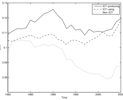
The era of ICT is also characterized by changes in the industrial organization and the institutional landscape. In this respect, one social aspect of ICT, namely its impact on skill-induced wage differentials, is discussed. As Figure 8 reveals, be-tween 1980 and 1990 the GINI-coefficient as a measure of wage dispersion bebe-tween low and high skilled labor rose sharply in the ICT-producing sectors due to the high demand of qualified workers, but decreased thereafter. Since 2000 the GINI-coefficient has been increasing again. With regard to ICT-using sectors, the GINI evolves along a similar path, though at a lower level and with an earlier peak in 1997. After 2000, the indicator decreased, but since 2003 it has shown an up-ward tendency again. Not surprisingly, the wage dispersion in Non-ICT-industries has declined significantly. Figure 9 links the evolution of wages of low and high skilled labor to the diffusion of ICT. A more sophisticated analysis would require econometric tools; however, as the empirical part of this paper focuses on the inter-sectoral linkages, comparing the development of ICT use among the different industries with the changes in wage dispersion of low and higher qualified work-ers suffices. To derive the diffusion pattern of ICT, again the compound direct requirements matrix (including imports and capital flows) is reverted to. As an indicator for dating the arrival of a GPT in a specific sector, following Jovanovic

and Rousseau (2005b) the year when the new technology reaches a one per cent

1980 1985 1990 1995 2000 2005 0.08

0.09 0.1 0.11 0.12 0.13

GINI

Time

ICT−producing ICT−using Non−ICT

Figure 8: Dispersion of wages of low and high-skilled labor between 1980 and 2005

technology. Another leap is observable before the dot.com-crash in 2000. As re-gards ICT-related services, particularly software, their diffusion follows the typical sigmoid path with a first bump in 1985 and a turning point after 1995. In the most recent years under study, both ICT manufacturing products and services have spread across the same range of sectors (about two third of all industries). Contrasting this diffusion pattern with the evolution of wage differentials, one can see that the wage dispersion peaked when the rate of adoption of ICT was about taking off in the mid 1990s. Interestingly, wage differentials between low and high-skilled labor have also increased significantly after 2000; at a time when the diffusion process had already slowed down and ICT begun to unfold its impact on labor productivity growth.

5

An evolutionary model of technological

diffu-sion

The time path of productivity measured by the maximum real wage ¯win equation (3) and the respective growth rategl

19650 1970 1975 1980 1985 1990 1995 2000 2005 2010 0.2

0.4 0.6 0.8

Diffusion

time

1965 1970 1975 1980 1985 1990 1995 2000 2005 20100.1 0.12 0.14

Gini

Diffusion ICS Diffusion ICM GINI

Figure 9: The diffusion of ICT manufacturing products (ICM) and ICT service products (ICS) across sectors (left ordinate) and the GINI-coefficient for low and high-skilled labor (right ordinate).

to understand the empirical results of the previous section. A thorough discussion of the underlying causes of the observed patterns is facilitated by a theoretical reconstruction of the observed data. Helpman and Trajtenberg(1996) andAghion

and Howitt (1998b) provide examples of how to explain on theoretical grounds

effects of the diffusion of innovative GPTs. Both modeling approaches include R&D activities as crucial in explaining observed patterns of the diffusion process, something which induces endogeneous technical change. It is possible to provide a sound theoretical explanation of output slump and transitory wage inequality by means of an evolutionary framework based on firm growth processes. To this end, the multi-sector formalism introduced in Section 2.1 is embedded into repli-cator dynamic equations. Time dependency of ¯w is therefore introduced since the technical coefficients change in time.

5.1

General model setting

The basic assumption is that for each sector n a number In of processes exists to

produce the respective good. At time t a fraction qin

is produced by processin. If ainmn is the input of good m and l in

nk the input of skill

k labor to produce one unit of goodn by means of process in, then

¯

anm = In X

i=1

qin

n a in

nm and ¯lnm= In X

i=1

qin

nl in

nm

are the respective input coefficients of the average technology defined by ¯A(t) and ¯

L(t). In this setting, (3) can be rewritten in a time-continuous manner as

¯

w(t) = 1 dT_[I−A¯_(t)]−1¯

L(t)u. (9) What remains to be answered is the time development of the market sharesqin

n

of the different technologies within their sector. Extra profits ρin

n gained by some

specific technology induce firm growth as follows. Assuming pricespto equal unit costs of production, they are implicitly given by

(1 +r+ρin

n)p T_ain

n +w(t)u T_lin

n =pn (10)

with vectors (ain

n,li

n

n) of input coefficients of technologyinin sectorn. Firm output

xin

n now grows according to extra profits. Consequently,

˙

xin

n

xin

n

=ρin

n

and due to xin

n =qi

n

nxn and ˙xn =

PIn

in=1x˙

in

n one gets ˙xn/xn= ¯ρn. Here xn denotes

total output of sectorn, and ¯ρn=PI

n

i=1qi

n

nρi

n

n is the average extra profit generated

in sectorn. Acknowledging ˙xin

n = ˙qi

n

nxn+qinnx˙n, the evolution of the system in the

presence of technical change is described by the replicator dynamics ˙

qin

n

qin

n

=ρin

n −ρ¯n. (11)

5.2

General Purpose Technology innovations: a two-sector

example

The introduced evolutionary multi-sector framework can be applied to the case of GPTs as follows. Technical progress due to a new GPT implies the existence of some new kind of technical device produced by a new (basic) sector. For the case of ICTs, let sector 1 be the one producing a commodity used for reproduction and for consumption. Prior to the existence of the new GPT, the economy is described by unit production input a1

11 and labor inputl11. As an aggregate of all

consumption commodities, this sector also serves as the num´eraire to express real wages w. At timet= 0, a new GPT is invented, leading innovating firms in sector 1 to introduce some new process characterized by

(1 +r+ρ2)(a211+a12p) +wul12 = 1 (12)

with unit production input a2

11 of the good itself and unit production input a12

of the GPT. ρ2 denotes the extra profits gained by the new process supported

by the GPT. Extra profit (respectively losses) ρ1 of the old technology are then

determined by

(1 +r+ρ1)a111+wl11 = 1. (13)

The new process needs high skilled labor remunerated by the wage premiumu >1. The GPT itself is produced in the new sector 2 according to

(1 +r)a2+wul22=p (14)

with capital input a2 from the incumbent sector 1 and high skilled labor inputl22,

yielding a pricep.

Equations (11-14) determine the dynamics of the system. For the special case of (a1

11, l11) = (0.3,0.3) and (a211, a12, l12) = (0.4,0.1,0.2) for the incumbent and

innovative process in sector n = 1 as well as (a2, l22) = (0.1,0.1) the diffusion

can also be observed, which is formally derived and graphically plotted in Figure

11based on expression (5) with

qh =

q(l12+a12l22)

(1−q)l11+q(l12+a12l22)

.

Also the slump after the innovation as a consequence of labor saving and cap-ital augmenting technological progress gets apparent in Figure 10. This is an illustration of Schumpeter’screative destruction in a more severe manner than he imagined: the decline of the incumbent process outperforms the rise of the innvoa-tion. As a consequence, output on average declines due to the destructive effect the innovation has on the incumbent technology.

0 −0.12 −0.1 −0.08 −0.06 −0.04 −0.02 0

Time

¯

ρ

Figure 10: Negative growth in case of a GPT innovation

6

Conclusion

The economic dynamics which is triggered off by the arrival of a general purpose technology is studied on both an empirical and theoretical level.

0

0 1

Time

0 10 20 30 40 50 60 700

0.005 0.01 0.015 0.02 0.025

q (left axis) GINI (right axis)

Figure 11: The diffusion of an innovative process and the resulting wage inequality.

just started, up to 2007. By accounting not only for the labor demand of a single industry, but also for the labor embodied in the upstream products, the derived labor productivity indicator gives more comprehensive insights into the impact of ICT on the economic system.

At the aggregate level, we have seen a falling trend of labor productivity par-ticularly over the last decades. Assessing the impact on overall growth within the whole period, the ICT-producing and ICT-using industries show an increasing contribution. However, it took two decades for ICT to become a major source of productivity growth, which indicates the long time span necessary for a GPT to reach maturity and for the economic system to adapt to the new technology. Comparing ICT to another general purpose technology, namely electricity, reveals that this sector has continuously lost in importance over time. This reflects the late stage in development of this GPT.

intensity. Furthermore, the distinction between an manufacturing and ICT-service sector allows tracking the different diffusion path of the related products. In this context, the final take-off of the ICT-manufacturing industry in the 1990ies was accompanied by a sharp rise in ICT services; this underpins the hypothesis that the diffusion of a GPT essentially depends on the development of complementary inputs that facilitate the switch from the old to the new technique. As regards the impact of ICT on the labor market, the diffusion of this technology can also be associated with transitional wage dispersion in the ICT-using industries.

Based upon this empirical evidence, ICT has been playing a crucial role in Denmark particularly in recent years, and given the current low growth rates of labor productivity, this role needs to be considered in future policy design.

As the second feature proposed by this article, the just described empirical results are reconstructed to some extent by an evolutionary multi-sectoral model. The retarded diffusion process and the induced transitional wage inequality are the two basic features which can be explained by the theoretical model. The former is a result of relative growth of innovative and non-innovative firms, and the latter is a consequence of skill premia, which are assumed to be paid for skills which are used for innovative production processes.

A

A.1

Structural decomposition analysis

Given Equation (8), the relative change in the maximum wage rate can be decom-posed into four partial factors: (1) technological change (as indicated by a change in the direct input matrixA, ∆S≡St−St−1), (2) change ∆l≡lt−lt−1of total

em-ployment, (3) substitution effect (indicated by a change in AT_{, ∆H ≡H}

t−Ht−1)

and (4) change ∆y ≡ yt−yt−₁ of final demand. The result of each

determinant to sectoral labor productivity growth:

SSt−1 ≡ −d

T

∆Sˆlt−1 [diag (Ht−1 yt−1)] −₁

wt e (15a)

llt−1 ≡ −d

T

St ∆ˆl[diag (Ht−1 y_t−1)] −1

wt e (15b)

LLt−1 ≡d

T

Stˆlt ˆx

−1

t [diag (∆H yt−1)] ˆx −1

t−1

wt e (15c)

Y Yt−1 ≡d

T

Stˆlt ˆx

−₁

t [diag (Ht ∆y)]ˆx

−₁

t−1

wte (15d)

Depending on data availability, the labor input is further decomposed into low-skilled (l1_{) and higher-skilled (l}2_{) labor (hours per unit of output).}

ll1t−₁ ≡ −d

T

St ∆ˆl1 [diag (Ht−1 yt−1)] −1

wt e (16a)

ll2_t−1 ≡ −d

T

St ∆ˆl2 [diag (Ht−1 y_t−1)] −1

wt e (16b)

Equations (16a-16b) replace (15c) for the time span of 1980 to 2005. Furthermore, final demand is decomposed into ICT-related and Non-ICT investments:

Y YICT t−1 ≡d

T

Stˆlt ˆx

−1

t [diag (Ht ∆yICT)]ˆx

−1

t−1

wte (17a)

Y YN onICT

t−1 ≡d

T

Stˆlt ˆx

−1

t [diag (Ht ∆yN on

−_ICT

)]ˆx−1

t−1

wte (17b)

Equations (17a) and (17b) sum up to (15d).

and taking the average of the two:

SSt≡ −dT

∆Sˆlt [diag(Htyt)]

−₁

wt e (18a)

llt≡ −dT

St−1 ∆ˆl[diag (H_t y_t)] −1

wt e (18b)

LLt≡dT

St−1ˆl_t−1 xˆ −1

t−1 [diag (∆H yt)

ˆ x−1

t ]wt e (18c)

Y Yt≡dT

St−1ˆlt−1 xˆ −₁

t−1[diag (Ht−1 ∆y)

ˆ x−₁

t ] wt e (18d)

Hence, the initial decomposition of the labor productivity growth indicator10_reads

as follows:

gtl=

1 2d

T

{(LLt−1+LLt}+{Y Y_t−1+Y Yt}+

{SSt−1 +SSt}+{ll_t−1+llt}

wt e

(19)

Inner- and intersectoral linkages

To show the impact of ICT on productivity changes across industries the direct input matricesAand AT _{are decomposed into their submatrices. FollowingMiller}

and Blair (2009, pp.603-605), changes in S and H are related to changes in the

underlying direct input matrices:

Proposition 1. Changes∆A of the input matrixA translate into changes ∆H of the Leontief Inverse and changes ∆S of the Sraffa Inverse according to

∆S=St−1 ∆A S_t and (20a)

∆H =Ht−1 ∆A

T_H

t. (20b)

Proof. (20b) is the transpose of (20a). Thus one only has to show that

(I−At)

−1

−(I−At−1) −1

= (I−At−1) −1

(At−At−1)(I−A_t) −1

.

10

For equations (15c) and (15d) as well as for equations (18c) and (18d), note that

ˆ x−_t1

−1∆ˆxˆx− 1

t =ˆx

−1

t ∆ˆxˆx

−1

t−1=−∆(ˆx−

1

)≡ˆx−_t1

−1−ˆx− 1

But this can be shown to be true by post-multiplication with (I−At) and

pre-multiplication with (I−At−1).

Analyzing the impact of a specific sector on all other sectors necessitates to take a closer look onto the economic structure. To assess how sectors are linked together, the direct input matrixAis split up in such a way that each row composes an own submatrix. By doing so, the isolated effect of one sector on the production technique can be traced back. Decomposing A into individual sectors means to create submatrices such that ∆A=PN

i=1∆A(i) with

∆A(i) ≡

        

0 . . . 0 . . . 0 ... ... ... ∆ai1 . . . ∆aij . . . ∆ain

... ... ... 0 . . . 0 . . . 0

         .

By recalling Proposition 1 and introducing ∆A(i) _{into equations (15a) and}

(18a), the effect of changes in the production process of a specific sector due to, for instance, technical change on labor productivity growth in all other sectors can be analyzed:

SSt ≡ −dT

h

St ∆A St−₁ˆl_t diag(H_ty_t) −1i

wt e

Applying the same procedure to equations (15c) and (18c) allows tracking the effect of changes in demand for a specific factor, i.e. the effect of substituting one input for another:

LLt=dT

h

St−1ˆl_t−1 xˆ −1

t−1 [diag (Ht ∆A

T _H

t−1 y_t)]ˆx −1

t

i

wt e

not captured within the direct input matrix, but are declared in the investment demand of an input-output table, so that for a comprehensive analysis changes in ICT-capital have to be taken into account in one way or the other. One possible approach is to re-weight the direct input-matrix by the share of fixed capital used in the production process. This implies the need for the so-called centre-coefficients for each sector, where the production recipe also represents capital assets and thus needs to be related to rates of profit. Another more simplistic approach that implies the incorporation of investment flows into the previous analysis is taken in this article to facilitate the empirical analysis: The final demand vector y is disentangled into different categories; furthermore the column of investment demand is replaced by the respective investment matrixY_{inv, which shows (similar}

to the industrial transaction matrix) the inner- and inter-sectoral deliveries of capital assets:

Y Yt−1 =d

T

[Stˆlt xˆ

−1

t [diag (Ht ∆(Y_inve+yrest))]xˆ

−1

t−1]wte

A.2

Industry classification

Table 2: Aggregation of Danish industries. Note: The numbers in the sec-ond column indicate the assignment of the respective sector to the Danish 130-industry-classification, the third column to ICT-producing, ICT-using and Non-ICT industries.

Code Industry Aggregation ICT-classification

1 Agriculture 1 Non-ICT

2 Horticulture, orchards etc. 2 Non-ICT 3 Agricultural services; landscape gardeners etc. 3 Non-ICT

4 Forestry 4 Non-ICT

5 Fishing 5 Non-ICT

Table 2 – continued from previous page

Code Industry Aggregation ICT-classification 14 Mfr. of rubber and plastic products 36-38 Non-ICT 15 Mfr. of other non-metallic mineral products 39-41 Non-ICT 16 Mfr. and processing of basic metals 42-47 Non-ICT 17 Mfr. of machinery and equipment n.e.c. 48-52 ICT-using 18 Mfr. of ICT equipment 53-55 ICT-producing 19 Mfr. of optical and medical equipment 56 ICT-using 20 Mfr. of transport equipment 57-59 ICT-using 21 Mfr. of furniture; manufacturing n.e.c. 60-62 Non-ICT 22 Electricity supply 63 Non-ICT 23 Gas and water supply 64-66 Non-ICT

24 Construction 67-70 Non-ICT

25 Sale and repair of motor vehicles etc. 71-73 ICT-using 26 Ws. and commis. trade, exc. of m. vehicles 74 ICT-using 27 Retail trade of food etc. 75 ICT-using 28 Department stores 76 ICT-using 29 Re. sale of phar. goods, cosmetic art. etc. 77 ICT-using 30 Re. sale of clothing, footwear etc. 78 ICT-using 31 Other retail sale, repair work 79 ICT-using 32 Hotels and restaurants 80-81 Non-ICT 33 Land transport; transport via pipelines 82-85 Non-ICT

34 Water transport 86 Non-ICT

35 Air transport 87 Non-ICT

36 Support. trans. activities; travel agencies 88-89 Non-ICT 37 Post and telecommunications 90 ICT-using 38 Financial intermediation 91-92 ICT-using 39 Insurance and pension funding 93-94 ICT-using 40 Activities auxiliary to finan. intermediat. 95 ICT-using 41 Real estate activities 96-98 ICT-using 42 Renting of machinery and equipment etc. 99 ICT-using 43 Computer and related activities 100-101 ICT-producing 44 Research and development 102-103 ICT-using 45 Consultancy etc. and cleaning activities 104-109 ICT-using 46 Public administration etc. 110-113 Non-ICT

47 Education 114-118 Non-ICT

References

Aghion, P., 2002. Schumpeterian growth theory and the dynamics of income in-equality. Econometrica 70 (3), 855–882.

Aghion, P., Howitt, P., 1998a. On the macroeconomic effects of major technological change. In: Helpman, E. (Ed.), General Purpose Technologies and Economic Growth. MIT Press, Cambridge, Ch. 5, pp. 121–144.

Aghion, P., Howitt, P., 1998b. On the macroeconomic effects of major technological change. Annales d’Economie et de Statistique, 53–75.

Allen, S., 2001. Technology and the wage structure. Journal of Labor Economics 19 (2), 440–483.

Basu, S., Fernald, J., 2007. Information and communications technology as a general-purpose technology: Evidence from US industry data. German Eco-nomic Review 8 (2), 146–173.

D. Autor, L. K., Krueger, A., 1998. Computing inequality: Have computers changed the labour market? Quarterly Journal of Economics 113, 1169–214. DeCicco, J., Fung, F., 2006. Global warming on the road. The climate impact of

America’s automobiles. Tech. Rep. 975, Environmental Defense Fund.

URL http://www.edf.org/sites/default/files/5301_

Globalwarmingontheroad_0.pdf

Degasperi, M., Fredholm, T., 2010. Productivity accounting based on production prices. Metroeconomica 61 (2), 267–281.

Dietzenbacher, E., Los, B., 1997. Analyzing decomposition analyses. In: Si-monovits, A., Steenge, A. E. (Eds.), Prices, Growth and Cycles. Macmillan, London, pp. 108–131.

E. Berman, J. B., Griliches, Z., 1994. Changes in the demand for skilled labor within US manufacturing industries. Quarterly Journal of Economics 109 (1), 367–398.

Helpman, E. (Ed.), 1998. General Purpose Technologies and Economic Growth. MIT Press, Cambridge.

Helpman, E., Trajtenberg, M., 1996. Diffusion of general purpose technologies. Tech. rep., National Bureau of Economic Research.

Helpman, E., Trajtenberg, M., 1998a. Diffusion of general purpose technologies. In: Helpman, E. (Ed.), General Purpose Technologies and Economic Growth. MIT Press, Cambridge, Ch. 3, pp. 85–119.

Helpman, E., Trajtenberg, M., 1998b. A time to sow and a time to reap: Growth based on general purpose technologies. In: Helpman, E. (Ed.), General Purpose Technologies and Economic Growth. MIT Press, Cambridge, Ch. 3, pp. 55–83. Inklaar, R., Timmer, M., 2007. Comparisons of industry output, inputs and

pro-ductivity levels. Economic Systems Research 19 (3), 343–363.

Jacob, J., 2003. Structural change, liberalization and growth: The Indonesian experience in an input-output perspective. Tech. rep., available athttp://www.

druid.dk/conferences/winter2003/Paper/jacob.pdf.

Jorgenson, D., Ho, M., Samuels, J., Stiroh, K., 2007. Industry origins of the Amer-ican productivity resurgence. Economic Systems Research 19 (3), 229–252. Jorgenson, D., Timmer, M., 2011. Structural change in advanced nations: A new

set of stylised facts. The Scandinavian Journal of Economics 113 (1), 1–29. Jovanovic, B., Rousseau, P. L., 2005a. General purpose technologies. Tech. Rep.

11093, National Bureau of Economic Research.

Jovanovic, B., Rousseau, P. L., 2005b. General purpose technologies. In: Aghion, P., Durlauf, N. (Eds.), Handbook of Economic Growth. Vol. 1B. Elsevier B.V., Ch. 18, pp. 1181–1224.

Koski, H., Rouvinen, P., Anttila, P., 2002. ICT clusters in Europe: The great central banana and the small Nordic potato. Information Economics Policy 14, 145–165.

Krueger, A., 1993. How computers have changed the wage structure: Evidence from microdata, 1984-1989. Quarterly Journal of Economics 108 (1), 33–60. Kurz, H., Salvadori, N., 1995. Theory of Production: A Long-Period Analysis.

Cambridge University Press.

Lenzen, M., 2003. Environmentally important paths, linkages and key sectors in the australian economy. Structural Change and Economic Dynamics 14, 1–34. Leontief, W., 1928. Die wirtschaft als kreislauf. Archiv f¨ur Sozialwissenschaft und

Sozialpolitik 60, 577–623.

Levy, F., Murnane, R., 1996. With what skills are computers complements? Amer-ican Economic Review 86 (2), 258–262.

Lipsey, R. G., Carlaw, K. I., Bekar, C. T., 2005. Economic Transformations. Gen-eral Purpose Technologies and Long-Term Economic Growth. Oxford University Press, New York.

Majumdar, S., 2008. Broadband adoption,jobs and wages in the us telecommuni-cations industry. Telecommunitelecommuni-cations Policy 32, 587–599.

McGowan, M. A., Jamet, S., 2012. Sluggish productivity growth in Denmark: The usual suspects? Tech. Rep. 975, OECD Economics Department Working Papers. Miller, R. E., Blair, P., 2009. Input-output analysis; Foundations and extensions.

Murphy, K., Welch, F., 1992. The structure of wages. Quarterly Journal of Eco-nomics 107, 255–85.

Nahuis, R., 2004. Learning of innovation and the skill premium. Journal of Eco-nomics 83 (2), 151–179.

Rainer, A., 2012. Technical change in a combined classical - evolutionary multi-sector economy, graz Schumpeter Centre Working paper No. 2.

Rose, A., Casler, S., 1996. Input-output structural decomposition analysis: a crit-ical appraisal. Economic Systems Research 8 (1), 33–62.

Sraffa, P., 1960. Production of Commodities by Means of Commodities. Prelude to a Critique of Economic Theory. Cambridge University Press, Cambridge. Yang, L., Lahr, M. L., 2008. Labor productivity differences in china 1987-1997:

An interregional decomposition analysis. The Review of Regional Studies 38 (3), 319–341.