A Model of Progressive Employee Compensation and Superstardom

(1)

A Model of Progressive Employee Compensation and

Superstardom

Susan Hamlen, William Hamlen, Lawrence Southwick School of Management, State University of New York at Buffalo, Buffalo, USA

Email: {mgthamle}@buffalo.edu

Received February 24, 2013; revised March 24, 2013; accepted April 24,2013

Copyright © 2013 Susan Hamlen et al. This is an open access article distributed under the Creative Commons Attribution License, which permits unrestricted use, distribution, and reproduction in any medium, provided the original work is properly cited.

ABSTRACT

This paper identifies the condition leading to a progressive salary situation wherein the elasticity of compensation with respect to ability is greater than unity, i.e., a small percentage advantage in ability results in a disproportional increase in compensation. This analysis also helps explain the “superstar phenomenon” made famous by Rosen (1981). Two as-sumptions are made. The first is that there is a generalized Cobb-Douglas type of production function wherein different hierarchies of employees of different abilities are viewed as distinct inputs. The second is that the distribution of ability is bell-shaped or approximately normally distributed, and can be approximated by a Poisson distribution. The model is applied using average outgoing salaries of MBA students from different universities compared to their average test scores.

Keywords: Progressive Salaries; Managers; Superstardom

1. Introduction

Our primary goal is to analyze the combined supply and demand factors that determine the elasticity of employee compensation relative to ability, where ability is assumed to be bell-shaped or normally distributed. Although the results are applicable to any occupation, we use the market for new managers as a relevant example. We attribute this application to early work by Rosen [1], who was interested in the progressive nature of managers’ salaries. Rosen [2] also introduced the “superstar phenomenon”, which seeks to explain why the top performers in many fields of endeavor, e.g., sports and music, receive compensation that is highly elastic with respect to ability. Progressive salary structures in the upper tail of the distribution of ability tend to result in highly skewed incomes in favor of the few most able managers. This, in turn, can cause social and political discontent.

In the second section below we present a brief over- view of the relevant literature. The third section intro- duces the Cobb-Douglas style production function assumed in the analysis. It, in turn, is used to generate demand functions for employees of any ability level. The fourth section identifies distributional assumptions concerning ability over the population of competing employees. The discrete Poisson distribution is used for mathematical convenience since it can be used to appro-

ximate a continuous normal distribution, and yields results that are easier to derive than those obtained by assuming a continuous distribution. The Poisson distribution of ability is combined with the demand functions from the third section to produce the final condition under which the progressive salary will exist. The fifth section applies the result to the relationship between average potential ability of graduating MBA (Master of Business Administration) students and their average outgoing salaries. As predicted by the model, the elasticity of compensation is greater than unity at higher levels of ability and less than unity at lower levels of ability. The sixth section summarizes our conclusions.

2. Literature Review

(2)

hierarchy managers. From a modeling perspective, having a distinct set of hierarchical positions implies that we cannot treat management as a single class of homogene- ous managers. Each level of the hierarchy must be viewed as a distinct factor of production. This also implies that there is a matching mechanism that efficiently allocates talent to the appropriate hierarchy.

The superstar phenomenon was defined by Rosen [2] as the situation where “small differences in talent become magnified into larger earnings differences, with great magnification if the earnings-talent gradient increases sharply near the top of the scale” (p. 846). He motivated the theory by describing how Alfred Marshall [3] was concerned with the distributional effects of a progressive salary structure with respect to ability, par- ticularly at the upper tail of the distribution for ability. The superstar concept has been applied to various economic situations in the entertainment industry, e.g., Scully [4], Jones and Walsh [5], Hamlen [6,7], Chung and Cox [8] and Lucifora and Simmons [9].

Murphy, Shleifer, and Vishny [10] (MSV) introduce a model of superstardom in the market for managers. They examine the situation where there are basically two hierarchies of management: one where less able managers receive a salary or wage based on standard marginal productivity conditions, and another where more able managers receive compensation based on some portion of the firm’s profits. They show that, in progressing from the lower management hierarchy to the higher management hierarchy, compensation can increase to an extent that is more than proportional to the manager’s differences in ability. Thus they considered this outcome an example of the “superstar phenomenon”. The MSV model provides a rationale for superstardom in the market for managers, but, as shown in this paper, the same phenomenon exists even if there is no hierarchy that receives a portion of the profits.

3. Production and Demand for Employees

We begin with an aggregate production function, written as a generalized Cobb-Douglas type production function.

  



1

i

m i i i

Y A H n 



 



(1)

In Equation (1), the output, Y, is the real GDP. The parameter “A

 

 ” incorporates both the state of technol- ogy and all inputs not under study, e.g., physical capital stock. The coefficients i,i1, , m, are the elasticities

of output relative to the increases in human capital stock,

i i, 1, , .

H n i  m These coefficients will be referred to as the production elasticities in order to distinguish these from the elasticities of salary or wage relative to a measure of ability, which is the primary interest of this paper.

Assume there are m distinct hierarchies of employees. In

of em

the hierarchical system described by Rosen these different hierarchies are treated as separate factors of production. Individuals seek employment in the highest hierarchy for which they may be considered, and the hiring agents for each hierarchy seek the potentially most able employees that are available. The variable Hi is a common

measure of the ability associated with individuals currently hired in hierarchy i, and ni is the number of such

individuals employed in that hierarchy. It must be em- phasized that each ni consists of the stock of existing

managers suited for that hierarchy. New additions to each hierarchy are relatively small in number relative to the existing stock of such employees. They accept the going wage rate for that hierarchy set by the supply and demand in the larger market of existing employees. This is basically the same as the assumption made in Witte’s [11] classic model for physical capital stock, where the larger market for existing capital stock determines the compensation rate in the smaller market for new capital stock.

We assume for convenience that the hierarchies ployees in Equation (1) are arranged from the lowest hierarchy, i1, to the highest level, i m . The product Hini becom approximate measure total amount

of human capital stock currently used in the ith hierarchy. We assume that as i approaches a continuum of hierar-

chies from i 1

es an of the

 to m, the difference between each i and i+1 become all, even though the difference between

1 and m may be quite significant.

Next, we make the usual assumpti s sm

on on employee hiring, that the salary of each individual in hierarchy i is based on the standard competitive model of optimal hiring within that hierarchy. The salary to the ith hierarchy em-ployee is equal to the value of the marginal product of the last individual hired in that hierarchy, or:

 













11

1

ˆ

, 1, , .

j i

i i i

m

j j i i i i

j i

i i i i i i

w  Y n n

A H n H n H

Y H n H Y n i m

 _ 

 



 

 

  

 

  





(2)

In Equation (2) the term Aˆ

r

implies that the other inputs are assumed to be at thei optimal values. In the final form of Equation (2), members of hierarchy i1 receive a higher salary than those of hierarchy i if i1i or

1

i i

n n



 or some combination of both. In o rds ages go to the employees in higher hierarchies if they have a higher production elasticity of output with respect to number of employees hired or if there are less individuals qualified to be employed in the higher hierarchy. The components i1

ther wo higher w

_ and _i are demand-side conditions for hiring in the pectiv ierarchy while the components n_i₁

res e h

 and ni are supply-side conditions. It is

useful to note at from quation (2) the ratio th E



w_i₁ w_i



,

(3)



wi1 wi

 

 i1 i



. Thus the ratio



i1 i



, which

appears throughout the paper, represents the ratio of “near intercepts” of the demand curves for employees in hierarchies i1 and i. When ni1 ni 1 we expect the

demand curve for employees of a greater hierarchy, i1, to have a greater intercept than that of the lower hiera , i. It follows that we expect

rchy



i1 i



1.

Equation (2) does not explicitly contain the measu ab

re of ility, Hi, but it is indirectly related since the number of

individuals in any employee hierarchy of level i will be determined by some probability distribution relating the level of ability, Hi, to the relative number of individuals, ni

that possess that ability level and are thereby included in that category. Therefore we can substitute n H_i

 

_i for ni

in Equation (2) producing:

 

i i i i

w Y n H (3)

4. The Distribution of Ability and Elasticity

A progressive wage or salary system exists when the elasticity of the wage or salary with respect to the measure of potential ability is greater than unity. The elasticity is above unity if the percentage change in the wage or salary, divided by the percentage change in the measure of ability, is above unity, or:



















 



1 1

1

or : 1 1

or : for all 1, , 1

i i i i i i i i i i i i i i

H H

w w H H

w w H H i m

 



 

   

  

   

(4)

Using Equation (3) for the wage on the left of Equation (4

w w w H

   

) the condition for the elasticity of wages with respect to the measure of ability to be above unity is:





 









 









1 1 1 1

, or :

i i i i i i i i

H

n H n H H H

 

   

 

  

 

(5)

Condition (5) crucially depends on the current number of

Y n H Y n H H

  

individuals, ni and ni+1 in adjacent hierarchies of employment. As noted above, Hi and ni are linked by some

distribution relating the measure of ability Hi to the

number of such individuals ni that have the required level

of ability to be hired in hierarchy i. A reasonable assumption is that ability among potential employees has a continuous bell-shaped distribution. In other words, there are relatively few with below average and above average ability but a large number with average ability. This is the assumption made by Neal and Rosen [12]. Such continuous distributions, however, seldom yield closed-form solutions and become difficult to analyze. Alternatively, since the Poisson distribution can be used to approximate a normal distribution, we approximate ability across the m hierarchies of employees using a discrete Poisson dis- tribution. Others have suggested that when using data for

only the very best employees, i.e., when only the upper tail of the normal distribution of ability is used, then the Yule-Simon distribution could be used, as it resembles the upper tail of the normal distribution. Appendix B contains the alternative results of this paper if that assumption is appropriate. For most situations, however, the Poisson probability function is preferred since it allows for bell-shaped distributions and can be used to approximate the normal distribution. Its probability density function is given by:

 

Prob Hiexp !, 1, 2, ,

i i

H  H H H i  m (6)

In the Poisson distribution there are m distinct hierarchies of employment and His the mean of the distribution. As the number of h archies becomes large, the discrete Poisson distribution approximates the normal distribution. If N is the total number of employees in all hierarchies of employment in a particular field, the predicted number of employees in each hierarchy i is:

ier

 

Prob

i i

n N H , where N is the total number of po- for all hierarchies. This allows us to substitute for ni and ni+1 on the left side of Equation (5). Thus for every i and i+1 in Equation (5) we have: tential employees

 

1

 

1 1

exp ! , 1, ,

and exp ! , 1, , 1

i H

 

  

i

i i

H

i i

n N H H H i m

n N H  H H i m

 

 

 

 

 _  _  

 



(7)

The measure of ability, H, can be treated as having ca

i

rdinal properties since we are interested in the elasticity and thus its percentage change. Here, for simplicity, we assume that the measure of ability takes on successive integer values such that Hi₁Hi1 for all i. This would be true for many mea an capital stock, e.g., discrete test scores, or years of education, or some measure of the quality of the education or training of an institution. Under this assumption, where Hi+1 and Hi

take on successive integer values, both



H H



1

sures of hum

1

i  i 

and

 

Hi1 Hi

H  _H

. In addition it is always true that



Hi1! Hi!



Hi1.

results of Equatio

Using these facts and substituting the n (7) into Equation (5), the elasticity of salary with respect to changes in the measure of ability,

S H  , is:



1







S H i i H Hi

  _  (8) We see from Equation (8) that the ratio of production elasticities,



i1 i



, is crucial to the resulting condition.

The ratio, as ove, is expected to be greater than one, but not highly greater than one if there are many hierarchies. Nevertheless, even if the ratio is close to unity a greater elasticity of salary or wage relative to ability will depend primarily on the ratio

noted ab

i

H H

 

 . In this case the ela-

(4)

S H

 , will always increase with increases in the hierarchy unde

rearranged in order to obtain the co

res of ab

r consideration. Equation (8) can be

ndition under which the elasticity, εS/H, will be greater

than unity, yielding the progressive salary result. Condition: For a system with discrete measu ility as described above, the condition that the elasticity of salary with respect to ability above unity is (Appendix A):



1



i i i

H    H (9) The condition (Equation (9)) th

co

at the elasticity of mpensation with respect to the measure of ability be greater than unity depends on the relative demand components,



 _i _i_₁



,and the mean of the distribution of ability, H . If there are many hierarchies, i1, , m, then it is expected that i1 and i are fair

value. In this situation t progressive salary schedule holds for any level of ability above the mean ability level ly close in he

H . When



 _i _i_₁



1 (the expected case) the pro- ssive sala exists at values of ability less than the mean

gre ry structure

H, and if under some condition we have



 i i1



1 i ccurs at values greater than the mean.

ly and demand conditions are required in tht o Both supp

re

5. An Application

city of compensation with respect

ple of

ates av

(10)

In Figure 1 the curved line within the data is based on pr

dition given by Equation (9), th

is sult. The elasticity of salary with respect to ability is above unity in the upper tail of the distribution of ability. Like the MSV model it qualifies as an example of the superstar phenomenon, but unlike the MSV model it does not require a separate hierarchy of employee that receives a share of profits rather than a higher salary based on the value of the marginal product within the hierarchy. The usual bell-shaped distribution of ability and a greater demand for more potentially able employees results in a progressive salary structure in the upper tail of the distribution of ability. This is also a condition which supports the superstar phenomenon with the minimum of assumptions concerning the distribution of ability and the demand for more able employees.

An example of the elasti

to ability can be observed by examining Stanford Uni- versity’s MBA program. In 2006 the average Graduate Management Admission Test (GMAT) score of entering students in all MBA programs was 560 [13] while the GMAT score for students entering Stanford’s MBA program was 720 [14]. Thus Stanford’s average GMAT score is approximately 29% higher than the national average. The average outgoing salary for all MBAs was $53,490 [15] while the average for Stanford was $165,500 [16]. The Stanford salary for graduating MBAs was approximately 209% above the national average. One measure of the elasticity of the differences between Stanford’s program and the national average is 7.22 (= 209%/29%).

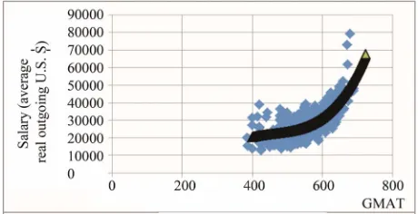
For a more inclusive analysis we make use of a sam 894 observations collected over seven years and 226 different MBA programs in the USA. The data is obtained from the various published editions of Miller [17]. As a measure of ability we use the average GMAT scores of entering students. A smaller sample of the data was ini- tially used by Hamlen and Southwick [18] to examine the relationship between input ability and output salaries for MBA programs. Figure 1 shows average outgoing salaries (all in real terms) plotted against average GMAT scores. From Figure 1 it is not difficult to predict that the elasticity of compensation with respect to ability will be higher for the upper level hierarchies of ability.

One convenient functional relationship that associ erage outgoing salary with average GMAT score is obtained by using a cubic regression of average salary as a function of GMAT score. The cubic regression adequately captures changes in slope and can be justified by the Stone-Weierstrass [19] theorem that states that any con-tinuous function can be approximated to any degree of accuracy by a polynomial of finite degree. Using a poly-nomial of degree greater than three results in strong mul-ticollinearity (_R2_{approaching 1). The result of the cubic} regression, wit _R2__0.62_{and t-values given in} paren-thesis, is:

Salary

h

   

2.81 3.54

2 3

4.10 4.87

184840 1368.18

2.92329 0.002119

GMAT

GMAT GMAT



  

 

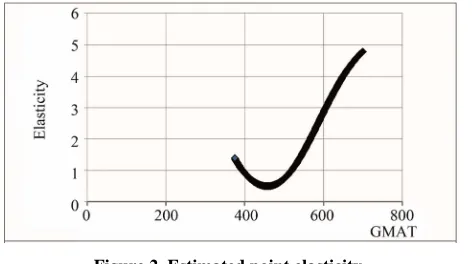
edicted salaries using Equation (9). In Figure 2, using Equation (10), the estimated point elasticity of salary with respect to GMAT score is calculated and plotted against the average GMAT score.

In agreement with the con

[image:4.595.308.538.601.719.2]

e elasticity is greater than unity for GMAT scores above the mean, GMAT = 560. The fact that the elasticity begins to exceed unity for values of GMAT scores slightly below the mean suggests, within the context of the above model, that



 i i1



1. We find that the results agree with the predictions of the model. The elasticity of average out-

(5)

[image:5.595.57.293.84.216.2]

Figure 2. Estimated point elasticity.

oing salary with respect to average GMAT score is ap-

ry structure with sp

6. Summary

assumptions regarding production and

s tested using average beginning salaries fr

REFERENCES

[1] S. Rosen, “A

g

proximately 0.49 for programs with below-average GMAT scores and approximately 1.77 for all programs with above-average GMAT scores.

As predicted, the progressive sala re- ect to potential ability becomes highly elastic (statisti- cally) when only the MBA programs with above-average GMAT scores are included, while those programs with below-average GMAT scores exhibit a low, inelastic relationship between compensation and potential ability. In essence, a greater demand for more able employees is matched with a smaller supply of such employees to produce a definite progressive salary in the upper tail of the distribution of potential ability.

Using standard

ability, and following Rosen’s [1] hierarchy structure, we find that progressivity of salary with respect to ability exists for employees with above average ability. Since it exists in the upper tail of the distribution of ability, this implies, as described by Rosen [2], that there is a superstar phenomenon. Within the same context, if only the upper tail of the normal distribution of ability is exam- ined and the Yule-Simon distribution [9] is appropriate, the progressive salary condition occurs for all hierarchies of employees.

The model wa

om various MBA programs in the USA and average test scores from the same programs. The elasticity of salary with respect to test scores was below unity for programs with below average test scores and above unity for programs with above average test scores. In addition the elasticity increases as the average test score increases.

uthority, Control, and the Distribution of Earnings,” The Bell Journal of Economics, Vol. 13, No. 2, 1982, pp. 311-323. doi:10.2307/3003456

[2] S. Rosen,“The Economics of Superstars,” The American

on,

rmance in Major League

. Walsh, “Salary Determination in

Economic Review, Vol. 71, No. 5, 1981, pp. 845-858.

[3] A. Marshall, “Principles of Economics,” 8th Editi MacMillan, New York, 1947.

[4] G. W. Scully, “Pay and Perfo

Baseball,” The American Economic Review, Vol. 64, No. 6, 1974, pp. 915-930.

[5] J. C. H. Jones and W. D

the National Hockey League: The Effects of Skills, Fran-chise Characteristics, and Discrimination,” Industrial and

Labor Relations Review, Vol. 41, No. 4, 1988, pp. 592-

604. doi:10.2307/2523593

[6] W. Hamlen, “Superstardom in Popular Music: Empirical Evidence,” The Review of Economics and Statistics, Vol. 73, No. 4, 1991,pp. 729-733. doi:10.2307/2109415 [7] W. A. Hamlen Jr. “Variety and Superstardom in Popular

Music,” Economic Inquiry, Vol. 32, No. 3, 1994, pp. 395- 406. doi:10.1111/j.1465-7295.1994.tb01338.x

[8] K. H. Chung and A. K. Cox, “A Stochastic Model of Superstardom: An Application of the Yule Distribution,”

The Review of Economics and Statistics, Vol. 76, No. 4,

1994, pp. 771-775. doi:10.2307/2109778

[9] C. Lucifora and R. Simmons, “Superstar Effects in Sport: Evidence from Italian Soccer,” Journal of Sports Eco- nomics, Vol. 4, No. 1, 2003, pp. 35-55.

doi:10.1177/1527002502239657

[10] K. M. Murphy, A. Shleifer and R. W. Vishny, “The Al- location of Talent: Implications for Growth,” The Quar-

terly Journal of Economics, Vol. 106, No. 2, 1991, pp.

503-530. doi:10.2307/2937945

[11] J. G. Witte, “The Microfoundations of the Social Invest- ment Function,” Journal of Political Economy, Vol. 71, No. 5, 1963, pp. 441- 456. doi:10.1086/258793

[12] D. Neal and S. Rosen, “Theories of the Distribution of Earnings,” In: A. B. Atkinson and F. Bourguignon, Eds.,

Handbook of Income Distribution, North-Holland, New

York, 2000, pp. 379-427.

doi:10.1016/S1574-0056(00)80010-X

[13] K. Schweitzer, “Taking the GMAT—GMAT Score,” 2006.

tarting Salaries at the Top Business

y Survey Report,” 2006.

h/US/Degree=Master of

.

/articles/biz/b

e to Graduate Business Schools,”

Output in MBA Programs: http://businessmajors.about.com/od/satgmatpreparation/a/ GMATscores.htm

[14] “Average MBA S Schools,” 2006.

http://www.admissionsconsultants.com/mba/compensatio n.asp

[15] “Salar

http://www.payscale.com/researc Business Administration (MBA)/Salary [16] “Admissions to Business Schools,” 2006

http://education.yahoo.com/college/essential school-admissions.html

[17] E. Miller, “Barron’s Guid

Barron’s Educational Series, Inc., Hauppauge, 1988, 1990, 1992, 1994, 1997, 1999, 2005.

[18] W. Hamlen and S. Southwick, “

Inputs, Outputs or Value Added?” Journal of Economic and Social Measurement, Vol. 15, No. 1, 1989, pp. 1-26. [19] M. Stone, “The Generalized Weierstrass Approximation

(6)

e general condition that the elasticity of respect to ability is greater than unity

Appendix A

In this appendix th compensation with is given by Equation (9).



i1 i



n Hi

 

i ni1



Hi1



 



Hi1 Hi



(A1) If the Poisson distribution of ability is assum given by Equations (6) and (7), Equation (A1) becomes:

ed and





₁



_



_

1

[ Hi exp !

i

1 1

exp !

i H

i

i i i i

N H H H

H H

  

   

  _{ }

  (A2)

N H  H H





 

 

Equation (A2) reduces to:











1



1! 1

i

i i i

! [

i

H H

i i H Hi H

  _ _  H H H

   (A3) This, in turn, reduces to:





1





1 1

i

i i i

1 i

H H

i i H   H H H (A4)

Given that and

eliminated from uatio obtain:

  

 

1

– 1

i i

H H  

both sides of Eq 1

0

i H  n (A4), we

can be





1

 

1 1

i i H Hi

  

    (A5) Finally rearranging Equation (A5) w

dition given by Equation (9).

we find that the Yule-Simon distribution ity of compensation relative to ability to e have the con-

Appendix B

In this appendix yields an elastic

be greater than unity as long as _i₁_i. The probability

density function for the Yule-Simon distribution is:

 









Pr Hi B Hi,1 ,0,Hi 1, 2, (B1)

and is the beta dist

s give y:



i, 1



B H 

This i n here b



, 1

 







B Hi   Hi1 ! !  Hi ! (B2) Substituting (B1) and (B2) into Equations (6) and (7) th



e condition that the elasticity of salary with respect to ability be greater than one becomes:









with 0 ribution.





_

_

_

_





1

1 1

1

1 !

1 ! ! 1 !

i i

H H



 

  



 



1 ! !

N  H  H

     

  

_ _

  

 

 



(B3)

Equation (B3) reduces to:





_



 

_{ }

1



_





1 1

1 !

1 1

i i

i i i i

i i

1 !

H H

 

 



 

  

  _

_ _{ } _{ } _

 

  (B4)

It further reduces to:

  

 



i1 i





1Hi



Hi1







Hi1 Hi



(B5) This yields the final result that assuming a Yule-Sim di

  _ _

on stribution of ability the condition that the elasticity of salary with respect to the measure of ability be greater than unity requires that:



i1 i



1



 Hi1



1 (B6)

Since we have assumed that



_i_₁ _i



1 and ρ and 1

i

H are both positive, then the salary with ct to ability is greater than unity for all i 1, ,m

elasticity of

respe   .

Thus if we assume that only the upper tail of l distribution is contained within the data set, and this can be approximated by a Yule-Simon distribution, then a progressive or superstar compensation system will exist at all levels of ability.