Munich Personal RePEc Archive
Estimation and Inference in Univariate
and Multivariate Log-GARCH-X Models
When the Conditional Density is
Unknown
Sucarrat, Genaro and Grønneberg, Steffen and Escribano,
Alvaro
BI Norwegian Business School, BI Norwegian Business School,
Universidad Carlos III de Madrid
11 August 2013
Estimation and Inference in Univariate and Multivariate Log-GARCH-X
Models When the Conditional Density is Unknown ∗
Genaro Sucarrat†, Steffen Grønneberg‡and ´Alvaro Escribano§
First version: 9 June 2010 This version: 23rd February 2015
Abstract
Exponential models of Autoregressive Conditional Heteroscedasticity (ARCH) are of special interest, since they enable richer dynamics (e.g. contrarian or cyclical), provide greater robustness to jumps and outliers, and guarantee the positivity of volatility. The latter is not guaranteed in ordinary ARCH models, in particular when additional exogenous and/or predetermined variables (“X”) are included in the volatility specifi-cation. We propose a general framework for the estimation and inference in univariate and multivariate Generalised log-ARCH-X (i.e. log-GARCH-X) models when the con-ditional density is not known. The framework employs (V)ARMA-X representations and relies on a bias-adjustment in the log-volatility intercept. The bias is induced by (V)ARMA estimators, but the remaining parameters are consistently estimated by (V)ARMA methods. We derive a simple formula for the bias-adjustment, and a closed-form expression for its asymptotic variance. Next, we show that adding exogenous or predetermined variables and/or increasing the dimension of the model does not change the structure of the problem. Accordingly, the univariate bias-adjustment is applicable not only in univariate log-GARCH-X models, but also in multivariate log-GARCH-X models. An empirical application illustrates the usefulness of the methods.
JEL Classification: C22, C32, C51, C52
Keywords: Log-GARCH-X, ARMA-X, multivariate log-GARCH-X, VARMA-X
∗An earlier version of this paper was entitled “The Power Log-GARCH Model”, seeSucarrat and
Escribano (2010). We are grateful to Jonas Andersson, Luc Bauwens, Christian Francq, Andrew
Harvey, Emma Iglesias, Sebastien Laurent, Enrique Sentana and seminar and conference participants at Nuffield College (Oxford University), Universit´e de Lille, Universidad Carlos III de Madrid, BI Norwegian Business School (Oslo), IHS (Vienna), 2nd. Rimini Time Series Workshop (2013), 21st. SNDE Symposium (Milan, 2013), ESEM 2011 (Oslo), Interdisciplinary Workshop in Louvain-la-Neuve 2011, CFE conference 2010 (London), FIBE 2010 (Bergen), IWAP 2010 (Madrid) and Foro de Finanzas 2010 (Elche) for useful comments, suggestions and questions. Funding from the 6th. European Community Framework Programme, MICIN ECO2009-08308 and from The Bank of Spain Excellence Program is gratefully acknowledged.
†Corresponding author. Department of Economics, BI Norwegian Business School, Nydalsveien
37, 0484 Oslo, Norway. Email [email protected], phone +47+46410779, fax +47+23264788. Webpage: http://www.sucarrat.net/
‡Department of Economics, BI Norwegian Business School. Email: [email protected].
§Department of Economics, Universidad Carlos III de Madrid (Spain). Email:
1 Introduction 2
2 Univariate log-GARCH 5
2.1 Notation and specification . . . 5
2.2 The ARMA representation . . . 6
2.3 On consistency . . . 6
2.4 On normality . . . 8
2.5 Log-GARCH-X . . . 9
3 Multivariate log-GARCH 10 3.1 Notation and specification . . . 10
3.2 The VARMA representation . . . 11
3.3 Multivariate log-GARCH-X . . . 12
4 Application: Modelling the uncertainty of electricity prices 13 4.1 Data . . . 13
4.2 Univariate log-GARCH models . . . 14
4.3 Multivariate log-GARCH models . . . 15
5 Conclusions 16
References 19
A Proof of Theorems 1 and 3 19
B Proof of Theorem 2 23
1
Introduction
The Autoregressive Conditional Heteroscedasticity (ARCH) class of models due to
Engle (1982) is useful in a wide range of applications. In finance in particular, it has been extensively used to model the clustering of large (in absolute value) finan-cial returns. Engle (1982) himself, however, originally motivated the class as useful in modelling the time-varying conditional uncertainty (i.e. conditional variance) of economic variables in general, and of UK inflation in particular. Other areas of ap-plication include, amongst other, the uncertainty of electricity prices (e.g. Koopman et al. (2007)), the evolution of temperature data (e.g. Franses et al. (2001)) and – more generally – positively valued variables, i.e. socalled Multiplicative Error Models (MEMs), seeBrownlees et al. (2012).
In fact, the greater the dimension of X, the more restrictions are needed in order to ensure positivity. Another desirable property is that volatility forecasts are more robust to jumps and outliers. Robustness can be important in order to avoid volatility forecast failure subsequent to jumps and outliers.
The log-GARCH class of models can be viewed as a dynamic version of Harvey’s (1976) multiplicative heteroscedasticity model, and was first proposed independently byPantula(1986),Geweke(1986) andMilhøj(1987). Engle and Bollerslev(1986) ar-gued against log-ARCH models because of the possibility of applying the log-operator (in the log-ARCH terms) on zero-values, which occurs whenever the error term in a regression equals zero. A solution to this problem, however, is provided in Sucarrat and Escribano (2013) for the case where the zero-probability is zero (e.g. because zeros are due to discreteness or missing values).1 The solution is only available when
estimation is via the (V)ARMA representation. Finally, two competing classes of exponential ARCH models are Nelson’s (1991) EGARCH and Harvey’s (2013) Beta-t-EGARCH model. The former has proved to be much more difficult theoretically (more on this below), and the latter is not – by its very nature – amenable to the assumption of an unknown conditional density (i.e. the conditional density must be known).
The assumption that the conditional density is unknown is particularly convenient from a practitioner’s point of view, since the user then does not need to worry about changing the conditional density from application to application, or alternatively to work with a sufficiently general density that will often make estimation and infer-ence numerically more challenging. This explains the attraction of Quasi Maximum Likelihood Estimators (QMLEs). In the univariate case consistency and asymptotic normality of QMLE for GARCH models under mild conditions were first established byBerkes et al. (2003) and Francq and Zako¨ıan(2004). In the exponential case most of the attention has been directed at Nelson’s (1991) EGARCH, whose asymptotic properties have turned out to be very difficult to establish, see e.g. Straumann and Mikosch (2006). Only recently was consistency and asymptotic normality proved (for the univariate EGARCH(1,1) only) under the complicated condition of contin-uous invertibility, see Wintenberger (2013). The log-GARCH model is much more tractable. Francq et al. (2013) prove consistency and asymptotic normality of the Gaussian QMLE for an asymmetric log-GARCH(p, q) model under mild conditions. Their method does not employ ARMA representations, which means it is more ef-ficient when the conditional error is normal or close to normal, but not when the conditional density is fat-tailed, see the asymptotic efficiency comparison in Francq and Sucarrat(2013)). Moreover, the estimator of Francq et al. (2013) cannot handle zero-errors or missing values as suggested in Sucarrat and Escribano (2013). Fi-nally, Francq and Sucarrat (2013) propose an estimator that achieves efficiency for conditional densities that are normal or close to the normal, by combining the ARMA-approach with the Centred Exponential Chi-Squared as instrumental QML-density. In the multivariate case, QML results have been established for the BEKK model of
Engle and Kroner (1995) by Comte and Lieberman (2003), for an ARMA-GARCH with constant conditional correlations (CCCs) byLing and McAleer(2003), for a
fac-1The same idea can be extended to the case where the zero-probability is non-zero and
tor GARCH model byHafner and Preminger (2009), for a multivariate GARCH with CCCs by Francq and Zako¨ıan(2010) and for a multivariate GARCH with stochastic correlations byFrancq and Zako¨ıan (2014) under the assumption that the system is estimable equation-by-equation.2 For exponential ARCH models there are no
mul-tivariate results. Kawakatsu (2006) has proposed a multivariate exponential ARCH model, the matrix exponential GARCH, which contains a multivariate version of Nel-son’s 1991 model. But there are no proofs for the estimation and inference methods that he proposes.
This paper makes four contributions. It is well-known that all the coefficients apart from the log-volatility intercept in a univariate log-GARCH specification can be estimated consistently (under suitable assumptions) via an ARMA representation, see for example Psaradakis and Tzavalis (1999), and Francq and Zako¨ıan (2006). However, the estimate of the log-volatility intercept will be asymptotically biased, and the bias is made up of a log-moment expression that depends on the unknown density of the conditional error. We propose a simple estimator of the log-moment expression that is made up of the empirical residuals of the ARMA regression, and derive an expression for its asymptotic variance (Sections 2.3-2.4). The practical consequence of this is that the log-volatility intercept can be estimated consistently, and hence thatall the log-GARCH parameters can be estimated consistently via the ARMA representation.
In the second contribution of our paper (Section 2.5), we show that the addition of exogenous, determinstic and/or predetermined conditioning variables, i.e. the log-GARCH-X model, does not alter the relation between the ARMA coefficients and the log-GARCH coefficients. So consistent estimation of the ARMA-X representation will produce exactly the same bias as earlier, and the bias correction procedure described above is applicable also for ARMA-X models.
In the third contribution (Section 3) we propose a multivariate log-GARCH-X model that admits time-varying conditional correlations. The model has a VARMA-X representation with a vector of error-terms. The vector is either IID, which cor-responds to the Constant Conditional Correlation (CCC) case, or independent but non-identical (ID), which corresponds to the time-varying correlations case. In both cases, however, each entry in the vector of errors is marginally IID. So the bias-correction from the univariate case can be used equation-by-equation – under suitable assumptions – subsequent to the estimation of the VARMA-X representation.
In the fourth contribution (Section 4) we illustrate the usefulness of our results by an application to the modelling of the uncertainty of electricity prices. Electricity prices are characterised by autoregressive persistence, day-of-the week effects, large spikes or jumps, ARCH and non-normal conditional errors that are possibly skewed. For robust (to jumps) forecasts of uncertainty (i.e. volatility) that accommodates all these characteristics, the log-GARCH-X model is particularly suited. The investiga-tion shows that volatility can be substantially underestimated if sufficient ARCH-lags and day-of-the-week effects are not accommodated.
The rest of the paper is organised as follows. The next section, section2, presents
2Jeantheau (1998) established general conditions for strong consistency for QML estimation of
the univariate log-GARCH model, the relation between the univariate log-GARCH model and its ARMA representation, and derives the log-moment estimator and its asymptotic variance. Also, it is shown that the addition of exogenous and predeter-mined variables does not alter the relationship between the log-GARCH and ARMA parameters. Section3shows how the ideas extend to the multivariate case. Section4
contains our empirical application, whereas Section5 concludes. Tables and Figures are placed at the end.
2
Univariate log-GARCH
2.1
Notation and specification
The univariate log-GARCH(p, q) model is given by
ǫt = σtzt, zt ∼IID(0,1), P(zt= 0) = 0, σt >0, (1)
lnσ2t = α0+
p
X
i=1
αilnǫ2t−i+ q
X
j=1
βjlnσ2t−j, t∈Z, (2)
where p is the ARCH order and q is the GARCH order. In finance, ǫt is often
interpreted as return or mean-corrected return, but more generally it is simply the error in a regression model. Throughout we will assume ǫt is observable and known.
Of course, this is not a realistic nor a desirable assumption, but simply reflects the current state of the theoretical literature.3 Denoting p∗ = max{p, q}, if the roots of
the lag polynomial 1−(α1+β1)L−· · ·−(αp∗+βp∗)Lp ∗
are all greater than 1 in modulus and if |E(lnz2
t)| <∞, then lnσt2 is stable. For common densities like the Student’s
t with degrees of freedom greater than 2, and the Generalised Error Distribution (GED) with shape parameter greater than 1, then σ2
t will generally be stable as well
if lnσ2
t is stable. Practitioners are often interested in the dynamics of other powers
than the 2nd., e.g. the 1st. power (i.e. the conditional standard deviation). For that purpose it should be noted that thedth. power log-GARCH(p, q) model can be written as
lnσdt =α0,d+ p
X
i=1
αiln|ǫt−i|d+ q
X
j=1
βjlnσtd−j, d >0, (3)
where α0,d = α0d/2. This means a complete analysis of the dth. power log-GARCH
model can be undertaken in terms of thed= 2 representation.
The log-GARCH model accommodates a broader range of persistency structures than the ordinary GARCH model. In particular, in contrast to the ordinary GARCH model, the unconditional autocorrelations of log-GARCH models depend on the dis-tribution ofzt: The more fat-tailed, the weaker correlations. Also, the log-GARCH is
capable of generating both weaker and stronger autocorrelations than the GARCH, and autocorrelation functions that decline either more rapidly or more slowly.
3To the best of our knowledge there are only two results in the literature that do not need to
2.2
The ARMA representation
If|E(lnz2
t)|< ∞, then the log-GARCH(p, q) model (1)-(2) admits the ARMA(p, q)
representation
lnǫ2t =φ0+
p
X
i=1
φilnǫ2t−i+ q
X
j=1
θjut−j +ut, (4)
where
φ0 =α0+ (1−
q
X
j=1
βj)·E(lnzt2), (5)
φi =αi+βi, 1≤i≤p, θj =−βj, 0≤j ≤q, (6)
ut = lnzt2−E(lnz2t). (7)
Consistent and asymptotically normal estimates of all the ARMA parameters – and hence all the log-GARCH parameters except the log-volatility interceptα0 – is thus
readily obtained via usual ARMA estimation methods subject to appropriate assump-tions, see e.g. Brockwell and Davis (2006). In order to obtain an estimate of α0 the
most common solutions have been to either impose restrictive assumptions regard-ing the distribution of zt (say, normality, see e.g. Psaradakis and Tzavalis (1999)),
or to use an ex post scale-adjustment (see e.g. Bauwens and Sucarrat (2010), and
Sucarrat and Escribano(2012)). What our argument below shows is that theex post
scale-adjustment (i.e. formula (8) below) provides a consistent estimate of E(lnz2
t).
Consequently, the final log-GARCH parameter,α0, can also be estimated consistently.
2.3
On consistency
To obtain an understanding of the motivation behind the scale-adjustment, consider writing (1) as
ǫt=σ∗tzt∗, zt∗ ∼IID(0, σz2∗),
where σ∗
t is a time-varying scale not necessarily equal to the standard deviation,
and where z∗
t does not necessarily have unit variance. Of course, by construction
σt =σt∗σz∗ and zt =zt∗/σz∗. Next, suppose a log-scale specification (e.g. an ARMA
specification contained in (4)) is fitted to lnǫ2
t, with lnσbt∗2 denoting the fitted value
of the ARMA specification such that bσ∗
t = exp(lnbσt∗), and with the ARMA residual
defined as ubt = lnǫ2t −ln ˆσ∗t2. In order to obtain an estimate of the time-varying
conditional standard deviation, which is needed for comparison with other volatility models, then it is natural to consider adjustingbσ∗
t by multiplying it with an estimate
ofσz∗, say, the sample standard deviation of the standardised residualszbt∗. Although
this argument is fine heuristically, it may not be apparent what underlying magnitude the adjustment in fact estimates, nor may it be straightforward to obtain the limiting properties of the adjustment under suitable conditions. In the log-GARCH model, however, the log of the scale-adjustment provides an estimate of −E(lnz2
this consider the scale adjustment and its approximation:
b
σz2∗ =
1
T −1
T
X
t=1
(zbt∗−zb∗t)2 ≈ 1
T
T
X
t=1
(zbt∗)2 = 1
T
T
X
t=1
exp(but).
The population analogue of the final expression on the right is E[exp(ut)]. Taking
the natural log of E[exp(ut)] gives lnE[exp(ut)] =−E(lnz2t) under the assumption
that E(z2
t) = 1, i.e. the identifiability assumption from (1). This suggests
−ln
"
1
T
T
X
t=1
exp(but)
#
(8)
provides a consistent estimate of E(lnz2
t) due to the continuity of the logarithm
function.
The expression in square brackets in (8), i.e. T−1P
t=T exp(ubt), is well-known as
the “smearing estimate”, seeDuan(1983). It provides an estimate of the adjustment needed for an unbiased estimate ofE(yt|xt) when the left-hand side of the estimated
model is lnyt.4 The proof of Duan(1983), however, is for static models. In dynamic
models, e.g. when the ubt’s are ARMA residuals, then a different proof strategy is
needed. Complete proofs under mild assumptions that hold under all the configura-tions covered in this paper, however, is well beyond our scope. For simplicity and convenience, therefore, we instead formulate the set of minimal assumptions and con-ditions that we rely upon throughout, and only provide a proof of the key condition (A2) in the log-ARCH(p) case.
Formally, we rely on the following assumptions:
A1: E(z2
t) = 1 and |E(lnzt2)|<∞.
A2: Let but, t= 1, . . . , T, denote the ARMA-residuals resulting from estimating the
ARMA representation (4). Then:
1
T
T
X
t=1
exp(ˆut)−
1
T
T
X
t=1
exp(ut) =oP(1). (9)
In A1 the first moment condition is simply the identifiability condition from (1), whereas the other moment condition|E(lnz2
t)|<∞ is required for the ARMA
rep-resentation (4) to exist. For the two most commonly used densities of zt in finance,
i.e. N(0,1) andt,E(lnz2
t) is finite. Regarding A2, it immediately implies that (8) is
a consistent estimator ofE(lnz2
t) due to the continuity of the logarithm function. As
we have already noted, though, a complete proof of A2 under all the configurations covered by this paper is beyond our scope. However, in the log-ARCH(p) case the proof is relatively straightforward.
Theorem 1. Suppose lnσ2
t = α0 +Ppi=1αilnǫ2t−i in (1)-(2), that lnǫ2t is strictly
stationary and that A1 holds. The mean-corrected AR(p) representation is then
4Specifically, if the estimated model is lnyt=β′x
t+ut with ut∼IID(0, σ2u), thenE(yt|xt) = E[exp(ut)]·exp(β′x
given by (lnǫ2
t −E(lnǫ2t)) =
Pp
i=1φi(lnǫ2t−i −E(lnǫ2t)) +ut, where φi = αi as in
(6). Define Yet = lnǫ2t −T−1
PT
t=1lnǫ2t. Let φb1, . . . ,φbp denote the OLS estimates of
φ1, . . . , φp based on the Yet’s, let ubt = Yet−Ppi=1φbiYet−i for t > p and let uet = 0 for
0< t≤p. If E(z4
t)<∞and |E[(lnzt2)2]|<∞, then A2 holds.
Proof. See Appendix A.
The Theorem states that A2 holds when the mean-corrected AR(p) representa-tion of a log-ARCH(p) model is estimated by OLS, which then implies that (8) is a consistent estimator of E(lnz2
t). Next, it follows straightforwardly that all the
log-ARCH(p) parameters can be estimated via the relationships (5) and (6), since
b
φ0 = (1−Ppi=1φbi)·T−1PTt=1lnǫ2t provides a consistent estimate of φ0 under the
assumptions of the Theorem. Strict stationarity of lnǫ2
t follows if the roots of the
AR-polynomial are all outside the unit-circle.
2.4
On normality
Our main interest is a consistent estimator ofE(lnz2
t), so that we can use the
ARMA-estimates to consistently estimate all the log-GARCH parameters via (5)-(6). To this end the limiting distribution of our estimator of E(lnz2
t) is of minor interest. In
simulations, however, the limiting distribution and an expression for the asymptotic variance can be useful in verifying simulation results.5
Let (8) be modified to
b
τT =−ln
"
1
T
T
X
t=1
exp(ubt−buT)
#
, (10)
where buT is the empirical mean of the ARMA-residuals. The mean-correction term
b
uT is needed, since condition A3 (below) may not be valid without it (see e.g. the
related discussion inYu(2007), where high moment partial sum processes of residuals in ARMA models are treated). Of course, in some cases, e.g. when OLS is used to estimate the AR(p) representation of a log-ARCH(p) model, then ubT is zero by
construction, and so (10) equals (8). The following two assumptions are needed for asymptotic normality:
A3: Let {but}Tt=1 denote the ARMA-residuals resulting from estimating the ARMA
representation (4). Denoting ubT and uT as the averages of ubt and ut,
respec-tively:
√ T
"
1
T
T
X
t=1
exp(but−ubT)−
1
T
T
X
t=1
exp(ut−uT)
#
=oP(1).
A4: E(z4
t)<∞ and |E[(lnzt2)2]|<∞.
5Of course, the limiting distribution is also useful for inference on E(lnz2
t), but this is not the
Condition A3 is slightly stronger than A2, since A3 implies that (10) provides a consistent estimate of E(lnz2
t) as long as A1 holds. The moment conditions in A4
are needed for the asymptotic variance of (10) to be finite.
Theorem 2. Suppose (1)-(2), A1, A3 and A4 hold. Then
√
TbτT −E(lnzt2)
D
−→N(0, ζ2), (11)
where
ζ2 =Var(zt2−lnz2). (12)
Proof. See Appendix B.
The key assumption for asymptotic normality to hold isA3, but a complete proof of it under all the configurations covered by this paper is beyond our scope. However, just as for consistency in the log-ARCH(p) case (see Theorem1), a proof of asymptotic normality in the log-ARCH(p) case is relatively straightforward.
Theorem 3. Suppose the assumptions of Theorem1 holds. If in addition E (u4
t) <
∞, then A3 holds.
Proof. See Appendix A.
AssumptionA4holds under the assumptions of Theorem1. The additional condition
E(u4
t)<∞ is in fact a very weak assumption, since it follows from E(e|ut|)<∞.
An extensive set of Monte Carlo simulations have been performed, of which Table
1only contains a small subset (more simulations are contained in Tables 2to 6, and additional simulations are available on request). The last three columns of Table 1
confirm that the Gaussian QMLE via the ARMA representation (w/mean-correction) provides consistent estimates and empirical sample standard errors that coincide with their asymptotic counterparts. Although, as expected, a larger number of observa-tions is needed as the persistence parameterφ1 =α1+β1 approaches 1, and when α1
goes towards zero (i.e. a common root). Additional simulations (available on request) show similar properties for the Gaussian QMLE without mean-correction, and for the Least Squares Estimator (LSE). All simulations and computations are inR (R Core Team (2014)) with thelgarch package (Sucarrat (2014b)).
2.5
Log-GARCH-X
Additional exogenous or predetermined variables (“X”) can be added linearly or non-linearly to the log-volatility specification lnσ2
t without affecting the relationship
be-tween the log-GARCH coefficients and the ARMA coefficients. Specifically, let the log-GARCH-X model be given by
lnσt2 =α0+
p
X
i=1
αilnǫ2t−i+ q
X
j=1
βjlnσt2−j+g(λ, xt), (13)
that all (or any) of its elements are contemporaneous. If |E(lnz2
t)| <∞, then (13)
admits the ARMA-X representation
lnǫ2t =φ0+
p
X
i=1
φilnǫ2t−i+ q
X
j=1
θjut−j +g(λ, xt) +ut, (14)
where the ARMA coefficients are defined as before, i.e. by (5)-(6), and where ut is
the same as earlier, i.e. ut = lnzt2 −E(lnzt2). Rigorous proofs of consistency and
asymptotic normality, which we do not provide here, would of course require precise assumptions on the behaviour of xt, see for example Hannan and Deistler (2012,
chapter 4). However, if all the ARMA-X parameters are estimated consistently, then a reasonable conjecture is that (8) provides a consistent estimate of E(lnz2
t), and
hence that all the log-GARCH parameters can be estimated consistently.
One type of conditioning variable that is of special interest in financial applications is leverage or volatility asymmetry. Table2provides simulation results that suggests Theorem 2holds for a simple version of leverage, namely
lnσt2 =α0+α1lnǫ2t−1+β1lnσt2−1+λ1I{zt−1<0}, (15)
where I{zt−1<0} is an indicator function equal to 1 if zt−1 <0 and 0 otherwise. Note
that I{zt−1<0} is observable, since I{zt−1<0} = I{ǫt−1<0}. The simulations suggest all
the parameters are estimated consistently, and the last three columns suggest the finite sample empirical standard errors of the estimate ofE (lnz2
t) correspond to their
asymptotic counterparts for both the normal and the t distributions. Additional simulations are contained in Table 5, where the univariate log-GARCH-X form is used equation-by-equation to estimate a multivariate log-GARCH(1,1) model with diagonal GARCH matrix and time-varying correlations.
3
Multivariate log-GARCH
3.1
Notation and specification
The M-dimensional log-GARCH model is given by
ǫt ∼ ID(0, Ht), t∈Z, (16)
D2t = diagσm,t2 , m= 1, . . . , M, (17)
zt = D−t1ǫt, ∀m:zm,t ∼IID(0,1), P(zt= 0) = 0, (18)
lnσ2t = α0 +
p
X
i=1
αilnǫ2t−i + q
X
j=1
whereǫt, σ2t andztare M×1 vectors, and whereHtand Dtare M×M matrices. In
(19) we have that α0 = (α1.0, . . . , αM.0)′,
αi =
α11.i · · · α1M.i
... . .. ...
αM1.i · · · αM M.i
and βj =
β11.j · · · β1M.j
... . .. ...
βM1.j · · · βM M.j
, (20)
where′ is the transpose operator. Equation (16) meansǫ
t is independent with mean
zero and a time-varying conditional covariance matrix Ht. The IID assumption in
equation (18) states that each marginal series {zm,t} is IID(0,1). Marginal
identi-cality is a key characteristic of the ARCH class of models, and is needed for (8) (or (10)) to be applicable after estimation via the VARMA representation. An implica-tion of (18) is that zt ∼ID(0, Rt), where Rt is both the conditional covariance and
correlation matrix – possibly time-varying – of zt. In other words, the vector zt is
ID but not necessarily IID, even though each marginal series {zmt} is IID. In the
special case where the vectorzt is IID, thenRt is a Constant Conditional Correlation
(CCC) model. Estimation of the volatilitiesD2
t does not require that the off-diagonals
of Ht (i.e. the covariances) are specified explicitly. Nor need we assume that ǫt is
distributed according to a certain density, say, the normal.
3.2
The VARMA representation
If|E(lnz2
t)|<∞, then the M-dimensional log-GARCH(p, q) model (19) admits the
VARMA(p, q) representation
lnǫ2t = φ0+
p
X
i=1
φilnǫ2t−i+ q
X
j=1
θjut−j +ut, (21)
where
φ0 =α0 + (IM − q
X
j=1
βj)·E(lnz2t), φi =αi+βi, θj =−βj and (22)
ut= lnzt2−E(lnzt2). (23)
In the special case where the vector zt is IID, which implies a CCC model for the
correlations (assuming they exist), then the vectorut is IID as well. In this case it is
well known that the multivariate Gaussian QMLE provides consistent and asymptot-ically normal estimates of the VARMA coefficients under suitable assumptions, see e.g. L¨utkepohl (2005). Accordingly, consistent estimation and asymptotically nor-mal inference regarding all the log-GARCH coefficients – apart from the log-volatility intercept α0 – is available as well. In order to obtain a consistent estimate of α0,
then an estimate of theM ×1 vector E(lnz2
t) is needed. Since the process {um,t} is
marginally IID for eachm, an equation-by-equation application of (8) (or of (10)) af-ter estimation of the VARMA representation is likely to provide consistent estimates of each element in E(lnz2
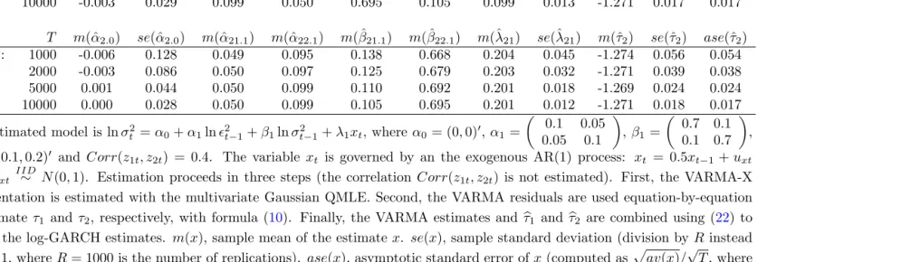
t). Tables 3 and 4 contain simulation results that support
columns suggest the empirical sample standard errors coincide with their asymptotic counterparts as implied by (12).
In the case where the vectorztis only ID, which is implied by time-varying
corre-lations, then the vectorut is only ID as well. This corresponds to a VARMA model
with heteroscedastic error ut. Fewer QML results are available in this case, e.g.
Bardet and Wintenberger(2009). However, in the special case where theβj matrices
are diagonal, then theM-dimensional VARMA model can be estimated equation-by-equation by univariate ARMA-X methods, since – equation-by-equation-by-equation-by-equation – each error term um,t is IID (along the lines of Francq and Zako¨ıan (2014)). Next,
equation-by-equation application of (8) is likely to provide consistent estimates of each element inE(lnz2
t), and hence of the log-volatility intercept α0. Table 5 contains simulation
results that supports this hypothesis when the time-varying correlations are governed by Engle’s (2002) Dynamic Conditional Correlations (DCC) model. The estimates of
α0andE(lnzt2) are consistent, and the last two columns suggest the empirical sample
standard errors coincide with their asymptotic counterparts as implied by (12).
3.3
Multivariate log-GARCH-X
Just as in the univariate case, the multivariate log-GARCH model permits exogenous and/or predetermined conditioning variables in each of theM equations. Specifically, write the multivariate log-GARCH-X specification as
lnσt2 =α0+
p
X
i=1
αilnǫ2t−i+ q
X
j=1
βjlnσt2−j+λxt, (24)
where xt is an L×1 vector of predetermined or exogenous variables, and where λ
is an M ×L matrix. Here, for notational economy, we let the predetermined or exogenous variables xt enter linearly, but in principle they can enter non-linearly as
in the univariate case, see (14). Similarly, the indext inxt does not necessarily mean
that all (or any) of its elements are contemporaneous. The VARMA-X representation of (24) is then given by
lnǫ2t = φ0+
p
X
i=1
φilnǫ2t−i+ q
X
j=1
θjut−j+λxt+ut,
with the VARMA coefficients and ut defined as before, i.e. by (22). In other words,
the relation between the VARMA coefficients and the log-GARCH coefficients are not affected by adding λxt to (24). So VARMA-X methods can be used to estimate
all the log-GARCH parameters (under suitable assumptions on xt) except the
log-volatility interceptα0 in a first step, and then in a second step equation-by-equation
application of (8) can be used to estimate each element in E(lnz2
t) and hence the
log-volatility intercept α0. Also here it is useful to distinguish between between the
CCC and time-varying correlations cases. If ut is IID, i.e. the CCC case, then –
can be estimated separately in terms of their ARMA-X representations.
4
Application: Modelling the uncertainty of
elec-tricity prices
Short-term electricity price modelling and forecasting is of great importance for en-ergy market participants. On the supply side, producers need forecasts of prices and the time-varying uncertainty associated with those forecasts in order to appropri-ately determine price and production levels. On the demand side, consumers and speculators need the same type of information to decide when and where to pro-duce, whether to speculate and/or hedge against adverse price changes, and for risk management purposes. Daily electricity prices are characterised by autoregressive persistence, day-of-the week effects, large spikes or jumps, ARCH and non-normal conditional errors that are possibly skewed. Koopman et al.(2007), Escribano et al.
(2011), and Bauwens et al.(2013) have proposed univariate and multivariate models that contain some or several of these features. However, in none of these models is the volatility specification – a non-exponential GARCH – robust to the large spikes that is a common characteristic of electricity prices (robustness is important to avoid large and persistent volatility forecast failure following spikes or “jumps”). Nor are they flexible enough to accommodate a complex and rich heteroscedasticity dynamics similar to that of the mean specification without imposing very strong parameter restrictions (e.g. non-negativity). Finally, automated model selection with a large number of variables is infeasible in practice due to computational complexity and positivity constraints. The log-GARCH-X class of models, by contrast, remedies these deficiencies. The objective of this section is to illustrate this.
4.1
Data
The data consist of the daily peak and off-peak spot electricity prices (in Euros per kw/h) from 1 January 2010 to 20 May 2014 (i.e. 1601 observations before lag-adjustments) for the Oslo region in Norway.6 Electricity forwards for this region is
traded at the Nord Pool Spot energy exchange, which is the leading European market for electrical energy. Factories, companies and other institutions with electricity con-sumption may want to shift part of their activity to and from peak hours for efficient cost management, since the difference between peak and off-peak prices can be very large at times, see Figure 1. As an aid in the decision-making process, forecasts of future prices and of price uncertainty (volatility) can therefore be of great usefulness. The daily peak spot price S1,t is computed as the average of the spot prices during
peak hours, that is,S1,t = (St(8am)+· · ·+St(9pm))/14, whereas the daily off-peak spot
price S2,t is computed as the average of the spot prices during off-peak hours, that
is, S2,t = (St(0am)+· · ·+St(7am)+St(10pm) +St(11pm))/10. Note that St(8am) should
be interpreted as the electricity price from 8am to 9am,St(9am) should be interpreted
6The source of the data ishttp://www.nordpoolspot.com/, and the sample was determined by
as the electricity price from 9am to 10am, and so on. Graphs of S1,t, S2,t and their
log-returns (rt = ∆ lnSt) are contained in Figure 1. The price and returns figures
exhibit the usual characteristics of electricity prices, namely that the price variability is substantially larger than those of financial prices (say, stocks, stock indices and exchange rates), and that big jumps occur relatively frequently.
4.2
Univariate log-GARCH models
The conditional mean is specified as a two-dimensional Vector Error Correction Model (VECM) augmented with day-of-the-week dummies in both equations.7 The residuals
or mean-corrected returns from the estimated model are then used for the estimation of the log-volatility specifications. The univariate models that we fit to each of the two mean-corrected returns are
log-GARCH(1,1) : lnσt2 =α0+α1lnǫt2−1+β1lnσt2−1, (25)
log-GARCH(7,1) : lnσt2 =α0+ 7
X
i=1
αilnǫ2t−i+β1lnσt2−1, (26)
log-GARCH(7,1)−X : lnσt2 =α0+ 7
X
i=1
αilnǫ2t−i+β1lnσt2−1+ 6
X
l=1
λlxlt, (27)
log-GARCH(7,1)−X∗ : lnσ12t=α0+ 7
X
i=1
α1.ilnǫ21,t−i+β1lnσ12,t−1+ 6
X
l=1
λlxlt
+
7
X
i=1
α2.ilnǫ22,t−i, (28)
log-GARCH(7,0)−X∗ : lnσ12t=α0+ 7
X
i=1
α1.ilnǫ21,t−i+
6
X
l=1
λlxlt
+
7
X
i=1
α2.ilnǫ22,t−i, (29)
whereǫt is the mean-corrected return in question, and wherex1t, . . . , x6t are six
day-of-the-week dummies for Tuesday to Sunday. In the last two specifications, where we add an asterisk ∗ to X, then ǫ
2,t is the mean-corrected off-peak return when ǫ1,t is
the mean-corrected on-peak return, and vice-versaǫ2,t is the mean-corrected on-peak
return whenǫ1,t is the mean-corrected off-peak return. Of course, this means the last
two equations could be considered as an Equation-by-Equation-Estimation (EbEE) scheme similar to that ofFrancq and Zako¨ıan(2014) (except that we do not estimate the time-varying correlations). The last specification, i.e. log-GARCH(7,0)–X∗,
actu-ally refers to a more parsimonious version than the one displayed. The parsimonious specification is obtained by automated General-to-Specific (GETS) model selection starting from (29), see Sucarrat and Escribano(2012).
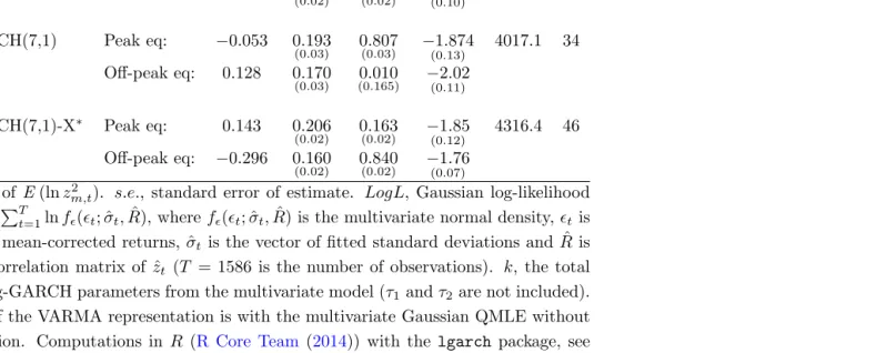
Table7contains the estimation results of the univariate models (only a selection of
7The R-squared of the two equations are 0.26 and 0.17, respectively. More details are available
the estimated parameters are reported for parsimony). The first striking characteris-tic of the results is the large ARCH(1) estimate of about 0.2 or just below for almost all the models. By contrast, daily financial returns typically exhibit an ARCH(1) estimate of about 0.05 (or lower). This means the uncertainty (i.e. volatility) of elec-tricity returns is much more volatile in comparison. Moreover, the estimate of about 0.2 does not change much if additional variables (e.g. lags of lnǫ2
t and day-of-the-week
dummies) are added. By contrast, the GARCH(1) termis affected when additional terms are added. In the plain log-GARCH(1,1) models, for example, it is estimated to 0.64 (peak) and 0.80 (off-peak), respectively. By contrast, when additional terms are added it falls – most of the time – to about 0 or close to 0. An interesting exception to this is the log-GARCH(7,1)-X∗ specification of the mean-corrected peak returns, and
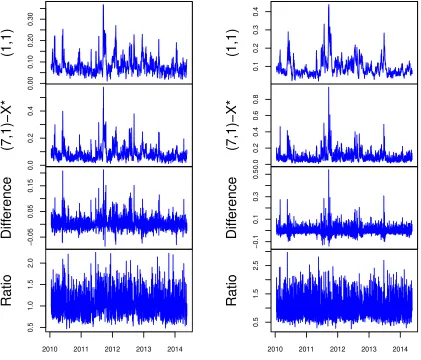
the log-GARCH(7,1)-X specification of the mean-corrected off-peak returns. Finally, Figure2 shows that the different specifications can produce fundamentally different volatility forecasts. In particular, the bottom graphs show that the log-GARCH(1,1) underestimates volatility on average, and that the log-GARCH(7,1)-X∗ models can
produce fitted standard deviations that are more than twice as big. In other words, one may seriously underestimate volatility if one does not properly take lags and day-of-the-week effects into account.
4.3
Multivariate log-GARCH models
The multivariate models that we fit to the vector of mean-corrected return ǫt are
m-log-GARCH(1,1) : lnσt2 =α0+α1lnǫt2−1+β1lnσt2−1, (30)
m-log-GARCH(7,1) : lnσt2 =α0+ 7
X
i=1
αilnǫ2t−i+β1lnσt2−1, (31)
m-log-GARCH(7,1)−X∗ : lnσt2 =α0+ 7
X
i=1
αilnǫ2t−i+β1lnσt2−1+λxt, (32)
where bothαi andβ1 are 2×2 matrices,xtis a 6×1 vector containing the six
day-of-the-week dummies andλis a 2×6 matrix. Table8contains the estimation results of the three multivariate models (again only a selection of the estimated parameters are reported for parsimony). Just as in the univariate case the ARCH(1) estimates are considerably higher than for daily financial returns – often close to 0.2, and they do not fall when additional terms are added. The m-log-GARCH(1,1)-X∗ estimates might
suggest that the model is not stable, since ˆα22.1 + ˆβ22.1 is very close to 1. However,
the roots of the lag-polynomial are in fact both outside the unit circle. Finally, also in the multivariate case is there sometimes a large difference between the fitted standard deviations. Specifically, just as in the univariate case, the plain multivariate log-GARCH(1,1) model may seriously underestimate the uncertainty (i.e. volatility) when compared with the multivariate model that also include lags and day-of-the-week periodicity in the volatility specification (i.e. m-log-GARCH(7,1)-X∗). This is
5
Conclusions
We have proposed a general and flexible framework for the estimation of and infer-ence in univariate and multivariate Generalised log-ARCH-X (i.e. log-GARCH-X) models when the conditional density is not known. Estimation is via the (V)ARMA-X representation, which induces a bias in the log-volatility intercept made up of a log-moment expression that depends on the conditional density. We proposed an esti-mator of the log-moment expression, and derived its asymptotic variance under mild assumptions. Due to the structure of the problem the bias-correction procedure is likely to also hold for univariate log-GARCH-X models, and – equation-by-equation – for multivariate log-GARCH-X models. An extensive number of simulations sup-port our conjecture. Finally, our empirical application shows that the methods are particularly useful when the volatility dynamics are complex and possibly affected by many factors.
The results in this paper suggests a vast range of new possible research ques-tions, both empirical and theoretical. Empirically, since the methods enable a much richer and flexible approach to volatility modelling in general – both univariate and multivariate, many problems that earlier could not be handled in practice due to computational complexity are now readily implemented. Theoretically, since estima-tion is via the (V)ARMA representaestima-tion, the vast literature on ARMA models and variants thereof serves as a source of ideas for possible extensions.
An early version of this paper (Sucarrat and Escribano(2010)) initiated the larger research agenda of which it is part. Sucarrat and Escribano(2012) relies explicitly on the results of this paper, whereasBauwens and Sucarrat (2010) is a precursor. These papers led to the development of the R (R Core Team (2014)) software packages
AutoSEARCH (Sucarrat (2012)) and gets (Sucarrat (2014a)) for automated General-to-Specific (Gets) modelling of ARCH-X models. An early critique of the log-ARCH class of models was that the log-log-ARCH terms in the log-volatility specification may not exist, since the errors of a regression in empirical practice can be zero. A solution to this problem, however, is proposed in Sucarrat and Escribano (2013). This solution is only available when estimation is via the (V)ARMA representation. Finally, Francq and Sucarrat (2013) propose another ARMA-based QMLE for log-GARCH models (with the centred exponential chi-squared as instrumental density) that is asymptotically more efficient when the conditional error is normal or close to normal.
References
Bardet, J.-M. and O. Wintenberger (2009). Asymptotic normality of the quasi maxi-mum likelihood estimator for multidimensional causal processes. Unpublished work-ing paper.
Bauwens, L., C. Hafner, and D. Pierret (2013). Multivariate Volatility Modelling of Electricity Futures. Journal of Applied Econometrics 28, 743–761.
Rate Volatility: A Forecast Evaluation. International Journal of Forecasting 26, 885–907.
Berkes, I., L. Horvath, and P. Kokoszka (2003). GARCH processes: structure and estimation. Bernoulli 9, 201–227.
Brockwell, P. J. and R. A. Davis (2006). Time Series: Theory and Methods. New York: Springer. 2nd. Edition, first published in 1991.
Brownlees, C., F. Cipollini, and G. Gallo (2012). Multiplicative Error Models. In L. Bauwens, C. Hafner, and S. Laurent (Eds.), Handbook of Volatility Models and
Their Applications, pp. 223–247. New Jersey: Wiley.
Comte, F. and O. Lieberman (2003). Asymptotic Theory for Multivariate GARCH Processes. Journal of Multivariate Analysis 84, 61–84.
Duan, N. (1983). Smearing Estimate: A Nonparametric Retransformation Method.
Journal of the Americal Statistical Association 78, pp. 605–610.
Engle, R. (1982). Autoregressive Conditional Heteroscedasticity with Estimates of the Variance of United Kingdom Inflations. Econometrica 50, 987–1008.
Engle, R. (2002). Dynamic Conditional Correlation: A Simple Class of Multivari-ate Generalized Autoregressive Conditional Heteroskedasticity Models. Journal of
Business and Economic Statistics 20, 339–350.
Engle, R. F. and T. Bollerslev (1986). Modelling the persistence of conditional vari-ances. Econometric Reviews 5, 1–50.
Engle, R. F. and K. F. Kroner (1995). Multivariate simultaneous generalized ARCH.
Econometric Theory 11, 122–150.
Escribano, A., , J. I. Pe˜na, and P. Villaplana (2011). Modelling Electricity Prices: International Evidence. Oxford Bulletin of Economics and Statistics 73, 622–650.
Francq, C. and G. Sucarrat (2013). An Exponential Chi-Squared QMLE for Log-GARCH Models Via the ARMA Representation.http://mpra.ub.uni-muenchen. de/51783/.
Francq, C., O. Wintenberger, and J.-M. Zako¨ıan (2013). GARCH Models Without Positivity Constraints: Exponential or Log-GARCH? Forthcoming in Journal of
Econometrics, http//dx.doi.org/10.1016/j.jeconom.2013.05.004.
Francq, C. and J.-M. Zako¨ıan (2004). Maximum likelihood estimation of pure GARCH and ARMA-GARCH processes. Bernoulli 10, 605–637.
Francq, C. and J.-M. Zako¨ıan (2006). Linear-representation Based Estimation of Stochastic Volatility Models. Scandinavian Journal of Statistics 33, 785–806.
Francq, C. and J.-M. Zako¨ıan (2014). Estimating multivariate GARCH and stochastic correlation models equation by equation. MPRA Paper No. 54250. Online athttp: //mpra.ub.uni-muenchen.de/54250/.
Franses, P. H., J. Neele, and D. Van Dijk (2001). Modelling asymmetric volatility in weekly Dutch temperature data. Environmental Modeling and Software 16, 131– 137.
Geweke, J. (1986). Modelling the Persistence of Conditional Variance: A Comment.
Econometric Reviews 5, 57–61.
Hafner, C. and A. Preminger (2009). Asymptotic theory for a factor GARCH model.
Econometric Theory 25, 336–363.
Hannan, E. and M. Deistler (2012). The statistical theory of linear systems. Philadel-phia, PA: Society for Industrial and Applied Mathematics (SIAM). Originally published in 1988 by Wiley, New York.
Harvey, A. C. (1976). Estimating Regression Models with Multiplicative Het-eroscedasticity. Econometrica 44, 461–465.
Harvey, A. C. (2013). Dynamic Models for Volatility and Heavy Tails. New York: Cambridge University Press.
Ibragimov, R. and P. C. Phillips (2008). Regression asymptotics using martingale convergence methods. Econometric Theory 24(4), 888–947.
Jeantheau, T. (1998). Strong consistency of estimators for multivariate arch models.
Econometric Theory 14, pp. 70–86.
Kawakatsu, H. (2006). Matrix exponential GARCH. Journal of Econometrics 134, 95–128.
Koopman, S. J., M. Ooms, and M. A. Carnero (2007). Periodic Seasonal REG-ARFIMA-GARCH Models for Daily Electricity Spot Prices. Journal of the
Amer-ican Statistical Association 102, 16–27.
Lee, S. (1997). A note on the residual empirical process in autoregressive models.
Statistics and Probability Letters 32(4), 405–411.
Ling, S. and M. McAleer (2003). Asymptotic theory for a vector ARMA-GARCH model. Econometric Theory 19, 280–310.
L¨utkepohl, H. (2005). New Introduction to Multiple Time Series Analysis. Berlin: Springer-Verlag.
Milhøj, A. (1987). A Multiplicative Parametrization of ARCH Models. Research Report 101, University of Copenhagen: Institute of Statistics.
Pantula, S. (1986). Modelling the Persistence of Conditional Variance: A Comment.
Econometric Reviews 5, 71–73.
Phillips, P. C. and V. Solo (1992). Asymptotics for linear processes. The Annals of Statistics, 971–1001.
Psaradakis, Z. and E. Tzavalis (1999). On regression-based tests for persistence in logarithmic volatility models. Econometric Reviews 18, 441–448.
R Core Team (2014). R: A Language and Environment for Statistical Computing. Vienna, Austria: R Foundation for Statistical Computing.
Straumann, D. and T. Mikosch (2006). Quasi-Maximum-Likelihood Estimation in Conditionally Heteroscedastic Time Series: A Stochastic Recurrence Equations Approach. The Annals of Statistics 34, 2449–2495.
Sucarrat, G. (2012). AutoSEARCH: General-to-Specific (GETS) Model Selection. R package version 1.2.
Sucarrat, G. (2014a). gets: General-to-Specific (GETS) Model Selection. R package version 0.2. http://cran.r-project.org/web/packages/gets/.
Sucarrat, G. (2014b). lgarch: Simulation and estimation of log-GARCH models.
Sucarrat, G. and ´A. Escribano (2010). The Power Log-GARCH Model. Universidad Carlos III de Madrid Working Paper 10-13 in the Economic Series, June 2010.
http://e-archivo.uc3m.es/bitstream/10016/8793/1/we1013.pdf.
Sucarrat, G. and ´A. Escribano (2012). Automated Model Selection in Finance: General-to-Specific Modelling of the Mean and Volatility Specifications. Oxford
Bulletin of Economics and Statistics 74, 716–735.
Sucarrat, G. and ´A. Escribano (2013). Unbiased QML Estimation of Log-GARCH Models in the Presence of Zero Returns. MPRA Paper No. 50699. Online athttp: //mpra.ub.uni-muenchen.de/50699/.
Wintenberger, O. (2013). Continuous Invertibility and Stable QML Estimation of the EGARCH(1,1) model. Scandinavian Journal of Statistics 40, 846–867.
Yu, H. (2007). High moment partial sum processes of residuals in ARMA models and their applications. Journal of Time Series Analysis 28, 72–91.
A
Proof of Theorems
1
and
3
We provide a common proof for both theorems, as they share much of the same structure.
Proof. We first note that we are here in the OLS case, which means that the residuals
estimator of φ:= (φ1, . . . , φp) based on mean corrected observations (Yt−Y¯T)1≤t≤T
where ¯YT = T−1PTt=1Yt. Let us write γ := Eeu0 and ˆγ = T1 PTt=1exp(ˆut). We
remind the reader that (ut) is assumed to be a zero mean IID sequence. In both
Theorem1and 3, we are given assumptionA3, which impliesVaru2
0 =E [(lnz12)2]−
[E ln(z2
1)]2 < ∞ as well as E exp(u1) = 1/(exp[E ln(z12)]) < ∞. When proving
Theorem 3, we are also given assumption A4, which implies that Var[exp(u1)] =
(Ez4
1−1)/({exp[E ln(z12)]}2)<∞, and soEe2u0 <∞.
Using this notation we see that Theorems 1 and 3 respectively follow from the following two cases which we will now show.
Case (i): If Eu2
0 < ∞ and Eeu0 < ∞ then ˆγ = γ +oP(1), i.e. ˆγ =T−1PTt=1exp(ut) +
oP(1).
Case (ii): IfEu4
0 <∞andEe2u0 <∞then
√
T(ˆγ−γ) =T−1/2PT t=1(eu
t−¯uT
−γ) +oP(1).
As a preliminary remark, we recall the standard result that √T( ˆφ′ −φ′) = OP(1)
under our assumptions (Brockwell and Davis,2006).
We first provide some expansions that will be useful for proving both case (i) and case (ii). Let δt,T := ˆut,T −ut. Note that δt,T = −ut when t ≤ p. We will for
notational simplicity omit theT subscript from both ˆut,T and δt,T in most cases. For
t ≤p we have euˆt = e0 = 1. We will see that these initial values are asymptotically insignificant and could be arbitrary. For the more interesting caset≥p+ 1, a Taylor expansion shows that
eut+δt =eut
+δteut+δ2t
Z 1
0
(1−x)eut+xδt
dx=eut
+δteut+eutδt2
Z 1
0
(1−x)exδt
dx. (33)
We are therefore interested in bounding δt, which we will do using a simple case of
the main argument in Theorem 1 ofLee (1997).
Letµ=EY0 =φ0/(1−Ppi=1φj). We have that ut=Yt−µ−Ppi=1φi(Yt−i−µ).
The definition of ˆut, as well as addition and subtraction shows that fort≥p+ 1, we
have that ˆut=ut−( ˆφ−φ)′(Yt−1−µ, . . . , Yt−p−µ)−T−1PTs=1(Ys−µ)(1−Ppi=1φˆi)
so that
δt,T =−( ˆφ−φ)′(Yt−1 −µ, . . . , Yt−p−µ)−T−1 T
X
s=1
(Ys−µ)(1− p
X
i=1
ˆ
φi). (34)
as in Lee (1997). Lee (1997) applies the so-called Phillips-Solo device (Phillips and Solo,1992) and concludes that
T−1/2
T
X
s=1
(Ys−µ) =
√
Tu¯T(1− p
X
i=1
φi)−1+ξT
with ξT = oP(1), see the proof of Theorem 1 in Lee (1997) immediately before his
eq.(2.6). Combining this with eq. (34) implies that for t≥p+ 1,
δt,T =−( ˆφ
′
whereRT =oP(T−1/2) does not depend on t. To see this, note that
√
T RT = (
√
Tu¯T)−(
√
Tu¯T)(1− p
X
i=1
φi)−1(1− p
X
i=1
ˆ
φi) +ξT(1− p
X
i=1
ˆ
φi)
Since√T( ˆφ−φ)′ =O
P(1) we have (1−Ppi=1φˆi) = (1−Ppi=1φi) +oP(1). Hence,
√
T RT = (
√
Tu¯T)−(
√
Tu¯T)(1− p
X
i=1
φi)−1(1− p
X
i=1
ˆ
φi) +ξT(1− p
X
i=1
ˆ
φi)
= (√Tu¯T)−(
√
Tu¯T)(1 +oP(1)) +oP(1) =oP(1),
where the last equality follows, since the central limit theorem implies that√Tu¯T =
OP(1). This implies that
MT := sup p+1≤t≤T|
δt,T| ≤ sup p+1≤t≤T|
( ˆφ′ −φ′)(Yt−1−µ, . . . , Yt−p−µ)|+|u¯T|+|RT|
= sup
p+1≤t≤T |
( ˆφ′−φ′)(Yt−1−µ, . . . , Yt−p−µ)|+|u¯T|+oP(T−1/2).
We have that
Tα sup
p+1≤t≤T|
( ˆφ′−φ′)(Yt−1−µ, . . . , Yt−p−µ)| ≤Tα sup
1≤j≤p|
ˆ
φj −φj| sup p+1≤t≤T|
Yt−µ|
=√T sup
1≤j≤p|
ˆ
φj−φj|Tα−1/2 sup p+1≤t≤T|
Yt−µ|.
We now recall that √T( ˆφ′−φ′) =OP(1). Also, because (Yt) is a strictly stationary
linear process with exponentially decreasing coefficients, it has the same number of moments as (ut) in the sense that Euκ0 < ∞ implies EY0κ < ∞ for any κ > 0.
Suppose 0≤α <1/2. It is a standard result that Tα−1/2sup
p+1≤t≤T |Yt−µ|=oP(1)
ifEu0−1/(α−1/2) <∞, see e.g. Lemma 12.4 ofIbragimov and Phillips (2008). For case (i), we knowEu2
0 <∞which corresponds toα= 0. For case (ii), we knowEu40 <∞,
corresponding to α= 1/4. For both of these possibilities, we see that
Tα sup
p+1≤t≤T|
( ˆφ′−φ′)(Yt−1−µ, . . . , Yt−p −µ)|=oP(1). (36)
Hence if Eu2
0 <∞, the assumption we may make under case (i), we conclude that
MT = sup p+1≤t≤T|
( ˆφ′−φ′)(Yt−1−µ, . . . , Yt−p−µ)|+|u¯T|+oP(T−1/2) =oP(1)
since T−1PT
t=1ut=oP(1) by the law of large numbers.
IfEu4
0 <∞, the assumption we may make under case (ii), we get
T1/4MT =T1/4 sup p+1≤t≤T|
( ˆφ′−φ′)(Yt−1−µ, . . . , Yt−p−µ)|+T−1/4|T1/2u¯T|+oP(T−1/4).
Because T1/2u¯
T =OP(1) by the central limit theorem, we see that T−1/4|T1/2u¯T| =
We now show consistency, i.e. case (i). Eq. (33) shows that 1 T T X t=1
euˆt = 1
T
p
X
t=1
euˆt +1
T
T
X
t=q+1
eut +1
T
T
X
t=q+1
δteut+
1
T
T
X
t=q+1
eut
δt2
Z 1
0
(1−x)exδt
dx, (37)
Clearly, T1 Ppt=1euˆt
= p/T = oP(1). We have that R01(1−x)exδtdx ≤ e|δt| because
for 0 ≤ x ≤ 1 we have (1−x) ≤ 1 and exδt
≤ e|xδt| = ex|δt|
≤ e|δt| so that R1
0(1−
x)exδtdx
≤ R01e
|δt|dx = e|δt|. By Eeu0 <
∞, the law of large numbers implies that
1
T
PT t=p+1eu
t
=Eeu0 +o
P(1). Hence, the triangle inequality implies that
|γˆ−γ| ≤ 1 T
T
X
t=p+1
|δt|eut +
1
T
T
X
t=p+1
eut
δt2e|δt|
+oP(1).
Using |δt| ≤MT we get that
|γˆ−γ| ≤MT
1
T
T
X
t=p+1
eut +M2
TeM
t1
T
T
X
t=p+1
eut
+oP(1).
which isoP(1) because MT =oP(1) and T−1PTt=p+1eut =Eeu0+oP(1) =OP(1).
Let us now show asymptotic Normality, i.e. case (ii). From eq. (33), we see that
√
T(ˆγ−γ) = √1
T
T
X
t=p+1
(eut
−γ)+√1
T
T
X
t=p+1
δteut+
1
√ T
T
X
t=p+1
eut
δt2
Z 1
0
(1−x)exδt
dx+oP(1)
The last sum isoP(1). To see this, we again use thatR01(1−x)exδtdx≤e|δt|combined
with the fact thatT1/4MT =oP(1) and we see that
1 √ T T X
t=p+1
eut
δ2t
Z 1
0
(1−x)exδt
dx ≤M 2
TeM
T 1
√ T
T
X
t=p+1
eut
=
T1/4
T1/4MT
2
eMT 1
√ T
T
X
t=p+1
eut
= (T1/4MT)2eMT
1
T
T
X
t=p+1
eut
,
which is oP(1) because (T1/4MT)2 = [oP(1)]2 = oP(1) by continuity, that eMT =
eoP(1)
=e0+o
P(1) = 1+oP(1) =OP(1), and by the law of large numbersT−1PTt=p+1eu
t =
OP(1).
We have therefore shown that√T(ˆγ−γ) = T−1/2PT
t=p+1(eu
t
−γ)+T−1/2PT
t=p+1δteu
t +
oP(1) =T−1/2PTt=1(eut−γ) +T−1/2PTt=p+1δteut+oP(1). To deal with the term
in-cludingδt, we apply eq. (35), which implies that
T−1/2
T
X
t=p+1
δteut =−( ˆφ
′
−φ′)T−1/2
T
X
t=p+1
(Yt−1−µ, . . . , Yt−p−µ)eut
−u¯T T−1/2 T
X
t=p+1
eut
!
+RTT−1/2 T
X
t=p+1
eut
Because Yt−j and ut are independent for j ≥ 0, we have that T−1PTt=p+1(Yt−1 −
µ, . . . , Yt−p−µ)eut =E [(Y−1−µ, . . . , Y−p−µ)eu0]+oP(1) = (0,0, . . . ,0)Eeu0+oP(1) =
(0,0, . . . ,0) +oP(1). Hence,
( ˆφ′−φ′)T−1/2
T
X
t=p+1
(Yt−1−µ, . . . , Yt−p−µ)eut =
√
T( ˆφ′−φ′)[(0,0, . . . ,0) +oP(1)],
which isoP(1) because
√
T( ˆφ′−φ′) = OP(1). RecallingRT =oP(T−1/2) implies that
RTT−1/2 T
X
t=p+1
eut
= (T1/2RT)T−1 T
X
t=p+1
eut
=oP(1)[Eeu0 +oP(1)] =oP(1).
We further have that
¯
uT T−1/2 T
X
t=p+1
eut
!
=√Tu¯T[Eeu0 +oP(1)]
=√Tu¯TEeu0 +oP(1)
√ Tu¯T
| {z }
=OP(1)
=√Tu¯TEeu0 +oP(1).
In conclusion, this shows that√T(ˆγ−γ) =T−1/2PT t=1(eu
t
−γ)−√Tu¯TEeu1+oP(1).
We now show that T−1/2PT t=1(eu
t−u¯T
− Eeu0) fulfils exactly the same expansion.
Indeed, we have thatT−1/2PT t=1(eu
t−u¯T
−Eeu0) = T−1/2PT
t=1e−¯u
Teut
−√TEeu0 =
e−¯uT
(T−1/2PT
t=1eu
t
)−√TEeu0
=e−u¯T
(T−1/2PT
t=1eu
t
−E eu0
+Eeu0
)−√TEeu0
=
e−¯uT(T−1/2PT
t=1[eu
t
−Eeu0]) +e−¯uT√TEeu0
−√TEeu0 = eoP(1)(T−1/2PT
t=1[eu
t
−
Eeu0
]) + [e−u¯T
−1]√TEeu0
. By the central limit theorem, which holds because we assume that Ee2u0 <
∞ we have that T−1/2PT t=1[eu
t
−Eeu0] = O
P(1) and hence
eoP(1)T−1/2PT
t=1[eu
t
−Eeu0] = (1 +o
P(1))T−1/2PTt=1[eut−Eeu0] =T−1/2PTt=1[eut−
Eeu0] +o
P(1)T−1/2PTt=1[eu
t
−Eeu0] = T−1/2PT
t=1[eu
t
−Eeu0] +o
P(1). The delta
method now implies that [e−u¯T
−1]√TEeu0
=√T[e−u¯T
−e0]Eeu0
=−√Tu¯TEeu0+
oP(1). The conclusion follows.
B
Proof of Theorem
2
Assumption A4 and the smoothness of the logarithm function imply that ˆτT and
˜
τT =−ln
" 1 T T X t=1
exp(ut−uT)
#
have the same behaviour up to oP(T−1/2). Denoting τ =E ln(z12) = −lnEeut, this
means√T(ˆτT −τ) =
√
T(˜τT −τ) +oP(1). Slutsky’s Theorem hence implies that we
only need show that ˜∆T =
√
T(˜τT −τ) is asymptotically normal. We have that
˜
τT =−ln
1
T
T
X
t=1
eut−¯uT
= ¯uT −ln
1
T
T
X
t=1
eut
so
˜ ∆T =
√ Tu¯T +
√ T " f 1 T T X t=1
eut
!
−f(Eeu1
)
#
,
wheref(x) =−lnx, withf′(x) =−1/|x|. By the smoothness off, the delta method
implies that
˜ ∆T =
√
Tu¯T +f′(Eeu1)
√ T " 1 T T X t=1
eut
−Eeu1
#
+oP(1)
= (f′(Eeu1
),1)√1
T
T
X
t=1
eut
−Eeu1
ut
+oP(1).
By the Multivariate Central Limit Theorem, we have that
1 √ T T X t=1
eut
−Eeu1
ut d −→ X Y ∼N 0 0 ,
Vareu1
Eu1eu1 Eu1eu1 Varu1
where we used thatEu1 = 0 andCov(u1, eu1) =Eu1eu1. Hence, ˜∆T d
−→f′(Eeu1
)X+
Y, which is mean zero normal with variance equal to
ζ2 = (f′(Eeu1
))2VarX+VarY + 2f′(Eeu1
)Cov(X, Y)
= Var[exp(u1)] [E exp(u1)]2
+Var(u1)−2
E[u1exp(u1)] E exp(u1)
.
Using the equalities
Var(u1) =E[(lnz21)2]−[E ln(z12)]2
Var[exp(u1)] =
1
{exp[E ln(z2 1)]}
2 ·(E z 4 1 −1)
E exp(u1) =
1 exp[E ln(z2
1)]
E[u1exp(u1)] =
1 exp[E ln(z2
1)] ·
E[(lnz21)z12]−E ln(z12)
we see that
ζ2 =E[(lnz12)2]−[E(lnz21)]2+ (E(z14)−1)−2E[(lnz12)z12] + 2E (lnz12)
From A4 we have that E(z4
1) < ∞ and E[(lnz12)2] < ∞. The Cauchy-Schwarz
inequality implies that |E[(lnz12)z12]|2 ≤ (E[(lnz12)2])(Ez14), so ζ2 is finite. Finally,
the expression simplifies to
Table 1: Finite sample properties of the Gaussian QMLE via the ARMA representation (w/mean-correction)
DGP (α0,α1,β1,τ)
T m(ˆα0) se(ˆα0) m(ˆα1) se(ˆα1) ase(ˆα1) m( ˆβ1) se( ˆβ1) ase( ˆβ1) m(ˆτ) se(ˆτ) ase(ˆτ)
zt∼N(0,1):
0,0.1,0.8,−1.27 1000 -0.020 0.056 0.101 0.023 0.022 0.783 0.065 0.053 -1.269 0.055 0.054 2000 -0.009 0.034 0.100 0.015 0.016 0.794 0.040 0.038 -1.270 0.038 0.038 5000 -0.003 0.020 0.100 0.010 0.010 0.797 0.024 0.024 -1.270 0.025 0.024 10000 -0.003 0.015 0.100 0.007 0.007 0.797 0.017 0.017 -1.268 0.016 0.017
0,0.05,0.9,−1.27 1000 -0.041 0.149 0.052 0.018 0.016 0.865 0.116 0.040 -1.272 0.054 0.054 2000 -0.011 0.032 0.050 0.012 0.012 0.891 0.036 0.028 -1.271 0.039 0.038 5000 -0.004 0.015 0.050 0.008 0.007 0.896 0.020 0.018 -1.270 0.024 0.024 10000 -0.004 0.011 0.050 0.005 0.005 0.897 0.012 0.013 -1.270 0.019 0.017
zt∼t(10):
0,0.1,0.8,−1.39 1000 -0.022 0.070 0.100 0.022 0.022 0.785 0.067 0.053 -1.390 0.059 0.061 2000 -0.008 0.038 0.101 0.015 0.016 0.792 0.041 0.038 -1.392 0.044 0.043 5000 -0.004 0.024 0.100 0.010 0.010 0.797 0.025 0.024 -1.388 0.028 0.027 10000 0.001 0.015 0.099 0.007 0.007 0.802 0.017 0.017 -1.389 0.018 0.019
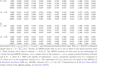
0,0.05,0.9,−1.39 1000 -0.025 0.076 0.051 0.018 0.016 0.879 0.068 0.040 -1.384 0.061 0.061 2000 -0.011 0.032 0.050 0.012 0.012 0.891 0.033 0.028 -1.389 0.043 0.043 5000 -0.004 0.017 0.050 0.007 0.007 0.896 0.019 0.018 -1.389 0.027 0.027 10000 -0.002 0.012 0.050 0.005 0.005 0.899 0.012 0.013 -1.391 0.021 0.019 The estimated model is lnσ2
t =α0+α1lnǫ2t−1+β1lnσ2t−1, and estimation proceeds in three steps. First,µ=E(lnǫ2t) is estimated
with the sample mean ˆµ=T−1PT
t=1lnǫ2t. Second, an ARMA-model withφ0 set to zero is fitted to the mean-corrected series
{lnǫ2
t−µˆ}. Third, formula (10) is used to estimateτ =E(lnzt2). The ARMA estimates are then used via the relationships (5)
and (6) to obtain the log-GARCH estimates. m(x), sample mean of the estimate x. se(x), sample standard deviation (division by R instead of R−1, where R = 1000 is the number of replications). ase(x), asymptotic standard error of x (computed as p
av(x)/√n, whereav(x) is the asymptotic variance ofx). The expressions ofav(ˆα1) and av( ˆβ1) are based on the ARMA(1,1) formulas inBrockwell and Davis (2006, pp. 259-260), whereas av(ˆτ) = ζ2, see (12). Computations in R (R Core Team (2014)) with a developer-version of thelgarchpackage, seeSucarrat(2014b).
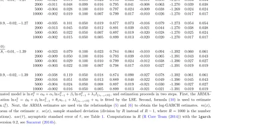
Table 2: Finite sample properties of the Least Squares Estimator (LSE) via the ARMA representation (without mean-correction) for a log-GARCH(1,1) with leverage
DGP (α0,α1,β1,λ1,τ)
: T m( ˆα0) se(ˆα0) m( ˆα1) se(ˆα1) m( ˆβ1) se( ˆβ1) m(ˆλ1) se(ˆλ1) m(ˆτ) se(ˆτ) ase(ˆτ)
zt∼N(0,1):
0,0.1,0.8,−0.01,−1.27 1000 -0.021 0.079 0.099 0.023 0.785 0.065 -0.011 0.088 -1.271 0.054 0.054 2000 -0.011 0.048 0.099 0.016 0.795 0.041 -0.008 0.063 -1.270 0.039 0.038 5000 -0.004 0.028 0.100 0.010 0.797 0.024 -0.009 0.038 -1.269 0.024 0.024 10000 -0.002 0.019 0.100 0.007 0.799 0.017 -0.010 0.026 -1.270 0.017 0.017
0,0.05,0.9,−0.02,−1.27 1000 -0.035 0.101 0.050 0.019 0.877 0.073 -0.016 0.079 -1.273 0.054 0.054 2000 -0.013 0.045 0.050 0.012 0.891 0.039 -0.021 0.044 -1.270 0.038 0.038 5000 -0.005 0.022 0.050 0.007 0.897 0.019 -0.020 0.028 -1.270 0.025 0.024 10000 -0.002 0.015 0.050 0.005 0.899 0.013 -0.020 0.020 -1.270 0.017 0.017
zt∼t(10):
0,0.1,0.8,−0.01,−1.39 1000 -0.023 0.079 0.100 0.023 0.784 0.064 -0.010 0.094 -1.392 0.060 0.061 2000 -0.009 0.050 0.100 0.016 0.793 0.039 -0.010 0.065 -1.391 0.043 0.043 5000 -0.001 0.029 0.100 0.010 0.799 0.024 -0.012 0.038 -1.390 0.027 0.027 10000 -0.003 0.022 0.100 0.007 0.798 0.017 -0.010 0.027 -1.391 0.019 0.019
0,0.05,0.9,−0.02,−1.39 1000 -0.038 0.119 0.050 0.018 0.874 0.090 -0.027 0.078 -1.392 0.061 0.061 2000 -0.016 0.051 0.050 0.013 0.889 0.040 -0.022 0.049 -1.390 0.045 0.043 5000 -0.004 0.024 0.050 0.008 0.897 0.019 -0.021 0.030 -1.390 0.027 0.027 10000 -0.002 0.016 0.050 0.005 0.899 0.013 -0.021 0.021 -1.391 0.019 0.019 The estimated model is lnσ2
t =α0+α1lnǫ2t−1+β1lnσt2−1+λ1I{zt−1<0}, and estimation proceeds in two steps. First, the
ARMA-representation lnǫ2
t = φ0+φ1lnǫ2t−1 +θ1ut−1+λI{zt−1<0} +ut is fitted by the LSE. Second, formula (10) is used to estimate τ = E(lnz2
t). Next, the ARMA estimates are used via the relationships (5) and (6) to obtain the log-GARCH estimates. m(x),
sample mean of the estimate x. se(x), sample standard deviation (division by R instead of R−1, whereR = 1000 is the number of replications). ase(ˆτ), asymptotic standard error of ˆτ, see Table 1. Computations in R (R Core Team (2014)) with the lgarch
package version 0.2, seeSucarrat(2014b).