An Autonomous Incremental Learning Algorithm
for Radial Basis Function Networks
Seiichi Ozawa1, Toshihisa Tabuchi1, Sho Nakasaka1, Asim Roy2
1
Graduate School of Engineering, Kobe University, Kobe, Japan; 2Department of Information Systems, Arizona State University, Tempe, USA
Email: [email protected], [email protected]
Received March 29th, 2010; revised September 14th, 2010; accepted September 17th, 2010.
ABSTRACT
In this paper, an incremental learning model called Resource Allocating Network with Long-Term Memory (RAN-LTM)
is extended such that the learning is conducted with some autonomy for the following functions: 1) data collection for initial learning, 2) data normalization, 3) addition of radial basis functions (RBFs), and 4) determination of RBF cen-ters and widths. The proposed learning algorithm called Autonomous Learning algorithm for Resource Allocating Network (AL-RAN) is divided into the two learning phases: initial learning phase and incremental learning phase. And the former is further divided into the autonomous data collection and the initial network learning. In the initial learning phase, training data are first collected until the class separability is converged or has a significant difference between normalized and unnormalized data. Then, an initial structure of AL-RAN is autonomously determined by selecting a moderate number of RBF centers from the collected data and by defining as large RBF widths as possible within a proper range. After the initial learning, the incremental learning of AL-RAN is conducted in a sequential way whenever a new training data is given. In the experiments, we evaluate AL-RAN using five benchmark data sets. From the ex-perimental results, we confirm that the above autonomous functions work well and the efficiency in terms of network structure and learning time is improved without sacrificing the recognition accuracy as compared with the previous version of AL-RAN.
Keywords: Autonomous Learning, Incremental Learning, Radial Basis Function Network, Pattern Recognition
1. Introduction
In general, when a learning model is applied to real-world problems, it does not always work well un-less a human supervisor participates initial settings such as choosing proper parameters and selecting the data preprocessing (e.g., feature extraction / selection and data normalization) depending on given problems. This dependence on human supervision is one of the highest barriers to wide deployment of artificial learn-ing systems. Therefore, removlearn-ing or alleviatlearn-ing human intervention in artificial learning systems is a crucial challenge. In fact, there have been proposed several approaches to autonomous learning [1-5].
On the other hand, the radial basis function network (RBFN) is one of the most popular models that has been applied to many applications such as pattern rec-ognition and time-series prediction [6]. Although RBFN has mainly been used as batch learning, the
sig-nificance of its extension to incremental learning is growing from a practical point of view [7,8]. Espe-cially, one-pass incremental learning [9] is an impor-tant concept for large-scale high-dimensional data. In this type of learning, the learner is required to acquire knowledge with a single presentation of training data (i.e., training data are never presented repeatedly for retraining purposes), and the learning must be carried out by keeping minimum information on past training data. Developing a stable one-pass incremental learn-ing algorithm for RBFN will give a great impact to many practical applications.
know, there is no online version of such an automated learning algorithm. This is because the distribution of training data is generally unknown in incremental learning environments where the data are only given in a sequential way. Besides, it is well known that the classifier performance could be affected by data pre-processing; especially, it could depend on whether data are normalized or not. As mentioned earlier, in most of the incremental learning algorithms, the parameter set-ting and the selection of a preprocessing method is conducted by an external supervisor on a trial and error basis when a learning algorithm is applied to a par-ticular problem. However, in incremental learning, this would sometimes be difficult for the supervisor if only a small number of training data are given in the begin-ning. Therefore, it is important to develop autonomous incremental learning algorithms so that a system can learn on its own without external help [12].
For this purpose, we have proposed an autonomous
learning algorithm for RBFN called Autonomous
Learning algorithm for Resource Allocating Network
(AL-RAN) [13]. AL-RAN is a one-pass incremental learning model which consists of the following auto-nomous functions: 1) data collection for initial learning, 2) data normalization, 3) addition of radial basis func-tions (RBFs), and 4) determination of RBF centers and widths. The first function enables AL-RAN to decide the necessity of data normalization from incoming training data, and if it is needed, the data scaling is autonomously carried out in an online fashion. And the third and fourth functions allow AL-RAN to free from tuning proper RBF centers and widths before the learning is started. In this AL-RAN model [13], train-ing data are first collected until both the mean and standard deviation are converged. Then, the average recognition accuracies for normalized and unnormal-ized data are evaluated using the leave-one-out cross-validation method. If the time evolution in rec-ognition accuracy becomes smaller than a threshold, the data collection is stopped and the necessity of data normalization is judged whether the accuracy for un-normalized data is significantly higher than that for normalized data. A problem in this algorithm is that the mean and standard deviation of collected data can largely be fluctuated over time depending on training sequences. Furthermore, evaluating the recognition accuracy at every learning stage would incur large computation costs.
In this paper, to alleviate the above problems, we propose to introduce the class separability instead of the recognition accuracy in a convergence criterion for data collection. The time to stop collecting data is de-termined by confirming the convergence of the class
separability or by finding the significant difference in the class separability for normalized and unnormalized data. In order to determine the initial structure of AL-RAN, a two-stage clustering algorithm is per-formed for the collected data to obtain a moderate number of prototypes and their cluster radii. These prototypes and radii are set to RBF centers and widths in AL-RAN, respectively. Then, the initial learning of AL-RAN is performed for the collected data to obtain connection weights and memory items in the long-term memory. After the above initial learning process, the learning is switched to the incremental learning phase and the learning is continued forever.
This paper is organized as follows. In Section 2, we first give a brief review of Resource Allocating Net-work with Long-Term Memory (RAN-LTM) [7,14] which gives a classifier model in AL-RAN, and then a new autonomous learning algorithm for AL-RAN is proposed in Section 3. Then, the performance of AL-RAN is evaluated for the five UCI data sets [15] in Section 4. Finally, conclusions and further work are described in Section 5.
2. Resource Allocating Network with
Long-Term Memory
us denote the number of inputs, RBFs, and outputs as I, J,
K, respectively. The learning algorithm of RAN-LTM is shown in Algorithms 1-3.
Let the inputs of a training data be x={x1, …, xI}’.
Then, the RBF outputs y={y1, …, yJ}’ are calculated as
follow:
2
2 || ||
exp j ( 1, , )
j
j
y j
x μ
J (1)
where jRI and j2 are the center and the width of the jth RBF. Let the weight from the jth RBF to the kth out-put be wkj and the bias of the kth output be k. Then, the
outputs z(x)={z1, …, zK}’ are given by ) , , 1 ( 1
K k
y w g z
J
j
k j kj
k
(2)
where
1
1
1
0
0
0
)
(
u
u
u
u
u
g
(3)The data in LTM are called memory items that corre-spond to representative input-output pairs. These pairs are selected from incoming training data, and they are learned with newly given training data to suppress for-getting. As seen in Algorithm 1, a memory item is cre-ated when an RBF is alloccre-ated; that is, a pair of an RBF center and the corresponding output is stored in LTM as a memory item.
The learning algorithm of RAN-LTM is divided into two phases: the addition of RBFs and the update of con-nection weights (see Algorithm 1). The procedure in the former phase is the same as that in RAN, except that
memory items are created at the same time. Once RBFs are allocated, the centers are fixed afterwards. Therefore, the connection weights W={wkj} are only parameters that
are updated based on the output errors. To minimize the errors, the following linear equation is solved [11]:
D
Φ
W (4) where D is the matrix whose column vectors correspond to the targets. Assume that a class c data (x, c) is given and J memory items (x~l,c~l) (l=1,…,J), where c~ is l
the class label of the l th memory item, are stored in LTM.
Then, the target matrix D is formed as follow:
1, , } ,
{ ~ ~
1 1 1
D
J c c
c . Here, 1c is a K-dimensional target
vector where the cth element is one and others are zeros. Furthermore, Φ{y(x),y(~x1),,y(~xJ)} are defined by the RBF outputs y for the training data and memory items. Using Singular Value Decomposition (SVD), is de-composed as follow: =UHV’. Then, the weight matrix
W in Equation (4) is given by the following equation:
D V H U
W
)
( (5)
where (H’)+ is the pseudo-inverse of H’.
3. Autonomous Incremental Learning
3.1. Assumptions and Learning SchemeLet us assume that no training data is given to a system in the beginning and training data are provided one by one. Since we expect a system to learn from incoming data with some autonomy, the learning system should collect training data on its own in order to determine an initial network with proper parameters, and then it should be able to improve the recognition accuracy consistently through incremental learning. To earn good performance, an autonomous learning system should judge whether some preprocessing (e.g., data normalization and feature extraction) is needed or not. As mentioned in Section 1, we consider only the data normalization for autonomous preprocessing. After the normalization, collected data are used for constructing and learning an initial AL-RAN classifier (i.e., RAN-LTM). The period up to this point is called initial learning phase.
After the initial learning phase, the incremental learning process is evoked. First, the data would be normalized if a system judges that the data normalization is preferable. Then, the incremental learning is conducted not only by updating network weights but also by allocating new RBFs and/or by updating the widths of existing RBFs. This period is called incremental learning phase.
3.2. Initial Learning Phase
3.2.1. Autonomous Data Collection and Normalization
autonomous learning system should collect training data. However, collecting too many training data leads to inef-ficiency in the computation and memory costs, and it also results in loosing the online learning property be-cause the autonomous system cannot make any predic-tion until such a large amount of data are collected. Therefore, it is important for a learning system to esti-mate a sufficient number of data for making a proper decision on the data normalization.
a) Previous Method: In the previous work [13], we proposed a heuristic method to determine the time to stop the data collection based on the following two criteria: the statistics of a data distribution (e.g., mean and stan-dard deviation) and the difference between the recogni-tion accuracies for normalized and unnormalized data (i.e., raw data). First, training data are collected until both the mean and standard deviation are converged. Then, the average recognition accuracy for normalized data Rnor and that for raw data Rraw are evaluated using the leave-one-out method. If the difference between the two recognition accuracies becomes smaller than a thre-shold r (i.e., | Rnor - Rraw | < r), the data collection is
terminated and the necessity of data normalization is judged; otherwise, more training data are collected until the above condition is satisfied. After satisfying the con-vergence condition, a system checks the significant dif-ference between Rraw and Rnor. If Rnor is not significantly lower than Rraw, the collected data are normalized such that they are subject to a normal distribution N (0,1), and all the data given in future are also normalized in the same way. Otherwise, the data normalization is not ap-plied not only to the collected data but also to training data given in future.
A problem of the above method is that the mean and standard deviation of collected data can largely be fluc-tuated over time depending on training sequences. If training data are uniformly drawn from a true distribu-tion, a relatively small number of training data would be sufficient to judge the convergence even with the above simple statistics. However, if training data are given based on a biased distribution, the mean and standard deviation of data would converge very slowly. Therefore, relying on only such simple statistics would result in increasing the average number of collected data.
A way to alleviate this problem is to introduce another stopping criterion. Recall that the purpose of the data collection is to judge the necessity of data normalization. Even though the data distribution does not converge, the data collection could be stopped when a system identifies a significant difference in the recognition accuracy for normalized and raw data. A straightforward way to im-plement this idea is to apply the cross-validation method at every learning stage. Obviously, however, large
com-putation costs are required for this. An alternative way is to adopt the class separability of data to estimate the recognition accuracy.
b) Proposed Method: Assume that n training data , where xi and ci, respectively corresponds to
the ith input and the class label, are collected so far. Let us further assume that the training data belong to either of C classes and the class c data set is denoted as
Xc= (c=1,…,C), where xciRI is the ith data of
class c and nc is the number of class c data. Then, the
whole input data set is denoted as . For the
collected data, the following between-class scatter matrix
SB and the within-class scatter matrix SW are defined: n
i i i,c)} 1 {(x
c n i ci} 1
{x
C c c} 1
{ X X 1 1 ( )( C
B c c c
c n n
S x x x x) (6)
1 1 1 ( )( c n C
W cj c cj
c j n
S x x x xc) (7)
where xc and x are the mean vectors of the class c
data and all data, respectively. The class separability Pn
for n training data is defined as follow:
}
{
tr
W1 Bn
P
S
S
. (8)This class separability Pn can be an alternative
meas-ure for the mean and standard deviation adopted in the previous work [13] because Pn includes the mean xc
and the total variance is defined by SB and SW. Therefore, Pn never converges unless both mean and standard
de-viation converge.
In this paper, we propose a new heuristic algorithm based on the class separability Pn, which could stop the
data collection with a moderate number of training data. Here, let us define the following difference Pn between
the class separability of unnormalized (raw) data Pnraw
and that of normalized data Pnnor:
raw nor
raw nor
|
max{ , }
n n n n n P P P P P
| . (9)
As a convergence criterion, we define the following average time-difference for Pn :
1
1 1
| 1
max{ , }
n k n k
n
k n k n k
P P P P P
|. (10)
In the previous work, the difference between the rec-ognition accuracies for normalized and raw data was adopted. This can be replaced with the difference Pn in
Equation (9). Thus, let us define another measure to ter-minate the data collection as follow:
1 1 k k n n PP . (11)
data collection. As seen in Algorithm 4, the class separa-bility is calculated for both raw and normalized data, and the average time-difference Pn is checked if it is smaller
than 2s. The reason why a large threshold 2s is used
here is to carry out a rough convergence check. After satisfying this condition, the second measure Pn is
checked if there is a significant difference between the class separability for normalized and raw data. Therefore, the data collection is terminated not only when the aver-age time-difference of the class separability Pn
con-verges but also when the average difference in the class separability for normalized and raw data Pn becomes
significant.
After terminating the data collection, the recognition accuracy for raw data Rraw and that for normalized data
Rnor are evaluated using the leave-one-out method. If Rraw
is significantly higher than Rnor, the collected data are used for learning RAN-LTM without normalization, and the data normalization is not also carried out for future training data. Otherwise, the normalized data are used for learning RAN-LTM, and the normalization is always applied to incoming data. Note that the cross-validation is carried out only once. In the following, for a notational convenience, let us express either normalized or raw data by X.
3.2.2. Initial Learning of AL-RAN
Training data collected in the
previous stage are used for the initial learning of AL-RAN, which is divided into the following two
proc-esses: determining an initial network structure and com-puting initial weights.
C c n i ci C c
c} 1 {{x }c1} 1
{
X
X
First, RBF centers are selected from X, and then prop-er RBF widths are detprop-ermined such that the RBF re-sponse fields cover all class regions with a moderate number of RBF centers. It is well known that in order to maximize the generalization performance, the number of RBFs should be as small as possible; therefore, an RBF width should be set as large as possible under the condi-tion that output errors are kept small. For this purpose, we propose an autonomous algorithm (Algorithm 5) to determine RBF centers and widths. The proposed algo-rithm consists of the following two stages: (1) rough se-lection of cluster centers (prototype candidates) and (2) selection of prototypes and determination of cluster radii.
In the first stage, the following procedures are carried out for every class c. First, the minimum distance dci*
between the ith data xci and other data xcj (j≠i) is
calcu-lated as follow:
cj ci i j ci
d
x
x
min
*
. (12)
Then, the minimum distances dci* are averaged over all
the class c data and the average value dc is calculated.
Since dc corresponds to the expected distance to the
nearest neighbors within a class c region, the rough se-lection is performed such that a prototype candidate ycj
represents several collected data within a cluster region whose radius should be set larger than dc. In order to
ensure that at least two data are represented by a proto-type in the rough selection, the radius is set to 2dc here.
As seen in Algorithm 5, the first prototype candidate yc1
is randomly selected from the collected data Xc= ,
and yc1 is put into the prototype candidate set Yc. Then, a
cluster region is defined such that yc1 is set to the center
and the radius is set to
c n i ci x } 1
{
c d
2 . Then, all the data within the region are represented by yc1, and they are removed from
Xc. The above procedures are continued until Xc becomes
empty.
In the second stage, prototype candidates are further selected to obtain prototypes by merging their cluster regions. As seen in Algorithm 5, the following procedures are carried out for every class c. First, a pro-totype candidate yci’ is randomly selected, and the
dis-tance to the nearest prototype of another class is calculated. Then, yci’ and dci* are respectively defined as
the first prototype pc1 and the cluster radius rc1. And all
the data within the cluster are removed from Yc. Such
procedures are continued until Yc gets empty. C c c} 1 {Y
* i c d
At the final stage of the initial learning, the structure of AL-RAN is initialized by creating RBFs and by com-puting weights. As seen in Algorithm 6, every pair of
prototype and the radius C is set to
c m i ci ci
RBF center j and RBF width j (j=1,…, J), respectively.
Here, J is the total number of RBFs (i.e., J
cC1mc).Then, the connection weights Wj from the jth RBF to the
outputs are computed as follow: Wj =1c - z(j) (j=1,…,J).
After initializing AL-RAN, all of the collected training
data 1 1 are given to AL-RAN one by one,
and AL-RAN is learned based on the same incremental
learning algorithm described in the next subsection (see Algorithm 7).
{{ } }nc C ci i c x
X
3.3. Incremental Learning Phase
In the incremental learning phase, the learning algorithm of AL-RAN is basically the same as that of RAN-LTM [7] except that RBF widths are automatically determined or adjusted in an online fashion. Let us explain how RBF widths are determined from incoming data. In pattern recognition problems, when an RBF center is near a class boundary, the RBF width is generally set to a small value in order to avoid serious overlaps between different classes. On the other hand, when an RBF center is lo-cated far from a class boundary, the width should be as large as possible to reduce the number of RBFs. How-ever, since only a part of training data are usually pro-vided at early learning stages, no valid information on class boundaries is generally given; thus, setting too large values to RBF widths could cause serious overlaps to other class regions at later learning stages, resulting in the catastrophic forgetting.
To avoid this, we adopt a safe strategy to determine the width of a newly created RBF. That is, the width of the J th RBF J is given by the distance to the closest
RBF center μj* as follow:
J j J j
Jmin μ μ
. (13)
In some cases, the closest RBF may have a large width that seriously overlaps with the support region of the new RBF. Therefore, the width of the closest RBF j* is
also resized as follow:
* min J * , *
j j j
The incremental learning algorithm of AL-RAN is sum-marized in Algorithm 7.
autonomous learning model. However, these parameters are relatively independent of given problems because normalized convergence criterions are adopted (see Equations (9-11)). Therefore, it is not difficult to set them properly.
3.4. Summary of Learning Algorithm and Intrinsic Parameters
The learning algorithm of AL-RAN is summarized in Algorithm 8. The initial learning phase is shown in Lines 2-5, and the remaining part corresponds to the incre-mental learning phase that could be repeated forever. Therefore, we can say that the proposed AL-RAN model is categorized into a lifelong learning model.
3.5. Discussions on Learning Convergence
Let us discuss the learning stability of AL-RAN by di-viding the learning algorithm into the three parts: 1) the initial learning phase (Algorithms 4-6), 2) incremental learning of individual training data (Algorithm 7), and 3) the main flow of the incremental learning phase (Algo-rithm 8).
Here, it should be noted that the inputs of Algorithm 8 are the parameters s, r, and that are used in the
auto-nomous data collection (see Algorithm 4). Although these parameters should be determined in advance, they are essentially different from so-called network parame-ters such as the number of RBFs and RBF widths which should be properly set depending on given problems. The above parameters mainly determine the behavior of an autonomous learning system.
As seen in Algorithm 4, the autonomous data collec-tion process would not stop if the two condicollec-tions at Line 15 are not satisfied forever. That is to say, the data col-lection could continue forever if the class separability of collected data does not converge or significant difference between the class separabilities for normalized and raw data is not detected. This can happen when the threshold s is too small and r is set too large. These thresholds
are called intrinsic parameters whose values are sup-posed to be set properly by an external supervisor. As long as these parameters are set properly, the data collec-tion would stop after a finite number of data are collected. However, it might not be easy even for a supervisor to set it properly under actual environments where the dis-tribution of training data is dynamically changed over time. Therefore, at the current version of AL-RAN, a perfect convergence for the initial learning phase is not theoretically guaranteed. However, as will be demon-strated later, the data collection always stops in our ex-periments (see Table 3). If the data collection stops, it means that the number of collected data is finite. Then, the other parts in the initial learning phase would termi-nate with finite operations (see Algorithms 5 and 6). As described in Section 3.2.1, the threshold s gives an
upper bound to judge the convergence of the class sepa-rability; thus, if s is set small, a strict convergence
crite-rion is applied, resulting in collecting many training data to make a decision. On the other hand, the threshold r
gives a lower bound of the separability difference be-tween normalized and raw data. Therefore, if r is set
small, this leads to a loose convergence criterion for the data collection. The parameter determines the period to monitor the degree of satisfying the convergence criteria. If is set small, a nearsighted convergence decision would be made, resulting in a loose convergence crite-rion. Hence, we can say that these parameters determine the behavioral property of an autonomous learning sys-tem. Let us call s, r, and intrinsic parameters.
In the current version of AL-RAN, such intrinsic pa-rameters should be set in advance by an external super-visor. In this sense, the proposed AL-RAN is not a fully
As seen in Algorithm 7, the learning algorithm of AL-RAN does not include iterative calculations that can continue forever. The weights are obtained with the ma-trix computation in Equation (5). In the augmentation of hidden units (RBFs), at most one hidden unit is created per training data. Therefore, the convergence of incre-mental learning for individual training data is ensured from the algorithmic point of view.
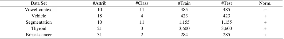
Table 1. Evaluated UCI Data sets. “Norm.” means the preference of data normalization: + means that data should be normalized.
Data Set
#Attrib #Class #Train #Test Norm.
Vowel-context
10 11 485 485 -
Vehicle
18 4234 423 +
Segmentation
10 11 1,155 1,155 +
Thyroid
21 3,6003 3,600 +
Breast-cancer
[image:8.595.55.541.216.443.2]31 2842 285 +
Table 2. The number of collected data and decision accuracy [%] for data normalization.
(a) Vowel-context
s
0.010.005 0.02 0.05
#Collected Data 43.264.6±15.7 31.2±11.7 22.8±7.1 ±5.0
0.1
Accuracy [%]
76 70 64 42
#Collected Data 47.165.8±15.2 34.0±13.7 25.9±9.0 ±6.5
0.25
Accuracy [%]
80 66 64 46
#Collected Data 64.299.0±25.0 43.2±16.2 27.4±11.7 ±6.3
0.5
Accuracy [%]
84 76 70 48
#Collected Data 64.699.0±25.0 43.2±15.7 27.4±11.7 ±6.3
r
1.0
Accuracy [%]
84 76 70 48
(b) Thyroid
s
0.010.005 0.02 0.05
#Collected Data 25.939.2±19.6 17.4±11.7 12.8±7.3 ±5.2
0.1
Accuracy [%]
88 94 88 84
#Collected Data 25.939.2±19.6 17.6±11.7 12.8±7.8 ±5.3
0.25
Accuracy [%]
88 94 88 84
#Collected Data 29.741.4±22.7 19.9±18.1 13.9±9.9 ±6.0
0.5
Accuracy [%]
92 96 90 84
#Collected Data 39.262.7±29.5 25.9±19.6 15.4±11.7 ±5.9
r
1.0
Accuracy [%]
90 88 94 82
routine of the incremental learning phase under such general learning environments.
4. Experiments
4.1. Experimental Setup
Five data sets are selected from UCI Machine Learning Repository [15] to evaluate the performance of AL-RAN.
Table 1 shows the information on the data sets. Al-though training and test data are separately provided in some data, they are merged and randomly divided into two subsets to conduct the two-fold cross-validation. Since the performance generally depends on the se-quence of cross-validation round (i.e., fifty sequences in total) are trained and the average performance is evalu-ated for the test data. We assume that training data are given one by one in a random order. The column ``Norm.'' in Table 1 shows the preference of data nor-malization: + means that the recognition accuracy is higher when the data is normalized. This preference was preliminary examined by evaluating the test performance of an RBF network which is learned with all the training data in a batch mode. Note that this preference is not
informed to AL-RAN.
The performance evaluation of AL-RAN is conducted through the comparison with the previous AL-RAN [13] and RAN-LTM. Let us denote the new and previous AL-RANs as AL-RAN(new) and AL-RAN(old), respec-tively. Here, we adopt the following performance meas-ures: 1) decision accuracy for data normalization, 2) the number of collected training data, 3) learning time, 4) the number of RBFs, and 5) final test recognition accuracy. The first measure is adopted to evaluate the autonomous data collection and the autonomous decision of data normalization in the initial learning phase. The decision accuracy is defined as the rate that the decision of the data normalization is matched with the preference in
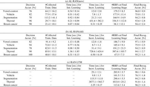
Table 3. Performance evaluations for (a) the proposed AL-RAN, (b) the previous AL-RAN, and (c) non-autonomous learning model RAN-LTM. The two values in each cell are an average value and the standard deviation in the form of x±y.
(a) AL-RAN(new) Decision
Accur. [%]
#Collected Train. Data
Time [sec.] for Init. Learning
Time [sec.] for Incre. Learning
#RBFs at Final Learning Stage
Final Recog. Accur. [%] Vowel-context
76 0.3464.2±16.2 12.0±0.14 179.3±2.0 96.8±8.3 ±0.9
Vehicle
82 0.5177.9±37.6 7.8±0.42 177.9±1.3 75.0±11.4 ±3.1
Segmentation
70 0.92113.2±61.1 21.2±0.84 166.9±4.4 94.2±14.9 ±0.8
Thyroid
96 0.2129.7±18.1 431.6±0.09 336.5±382.3 93.6±112.0 ±2.8
Breast-cancer
98 0.0721.4±10.1 0.31±0.04 38.1±0.25 94.4±12.1 ±2.4
(b) AL-RAN(old) Decision
Accur. [%]
#Collected Train. Data
Time [sec.] for Init. Learning
Time [sec.] for Incre. Learning
#RBFs at Final Learning Stage
Final Recog. Accur. [%] Vowel-context
82 1.1391.4±9.2 12.8±0.48 186.7±1.8 97.1±9.0 ±0.9
Vehicle
94 0.7772.8±11.3 8.7±0.36 185.4±1.2 75.9±9.1 ±2.5
Segmentation
78 0.9882.0±11.3 31.4±0.50 191.2±9.1 94.2±21.5 ±0.9
Thyroid
90 1.3685.0±13.1 728.6±1.83 387.6±624.4 94.1±103.7 ±2.7
Breast-cancer
100 0.3140.8±10.1 0.50±0.13 47.5±0.19 95.2±7.3 ±1.4
(c) RAN-LTM Decision
Accur. [%]
#Collected Train. Data
Time [sec.] for Init. Learning
Time [sec.] for Incre. Learning
#RBFs at Final Learning Stage
Final Recog. Accur. [%]
Vowel-context - - - 25.1±2.1 203.9±5.7 98.1±0.6
Vehicle - - - 9.8±1.3 161.5±5.1 76.3±1.8
Segmentation - - - 115.5±11.0 290.4±5.5 94.2±0.8
Thyroid - - - 3877.1±563.7 653.0±25.2 91.8±1.4
Breast-cancer - - - 2.25±0.17 113.6±3.4 96.2±1.0
4.2. Effects of Intrinsic Parameters
Before evaluating the performance of AL-RAN, let us examine how the intrinsic parameters affect the behavior of AL-RAN. As described in Section 3-4, and r have a
similar effect on the model behavior. Hence, we only study the influence of s and r for simplicity. In the
fol-lowing experiments, is fixed at 5.
Tables 2 (a) and (b) show the number of collected data and the decision accuracy in the initial learning phase for (a) Vowel-context data and (b) Thyroid data. As seen in Tables 2 (a) and (b), when s is getting small,
the number of collected data is increasing and the deci-sion accuracy for data normalization becomes high. The same is true when r is getting large. Although this is not
a surprising result, an interesting interpretation is that these intrinsic parameters control the discretion of a sys-tem. That is, a system with a smaller s would be more
discreet to make a decision, while a system with a smaller r would become more optimistic.
4.3. Performance Evaluation
Table 3 shows the decision accuracy for data normaliza-tion, the number of collected data in the initial learning phase, the time required for initial learning and
incre-mental learning, the number of RBFs, and the test recog-nition accuracy after all the learning is completed. The parameters used in the experiments are r= 0.5 and s =
0.01. For a comparative purpose, we also evaluate two incremental learning models. The one is the previous AL-RAN model (AL-RAN(old)) which adopts different convergence criteria on the data collection and a differ-ent method to initialize AL-RAN in the initial learning phase (see [13] for details). The other is RAN-LTM in which a fixed RBF width is given and the data normali-zation is determined based on the preference shown in
Table 1; that is, the learning of RAN-LTM is not auto-nomously carried out.
time for initial leaning is shortened. This is because the convergence for data collection is checked based on the class separability whose computation costs are smaller than those for the cross-validation in AL-RAN(old).
The experimental results for the five UCI data sets demonstrate that although the decision accuracy for data normalization is relatively lower than the previous AL-RAN model, the number of collected data is de-creased and the time for the initial learning is also short-en. From the fact that the test recognition accuracy of the proposed AL-RAN is not degraded significantly after all incremental learning is completed, the degradation in the decision accuracy for the data normalization is not a critical problem. Therefore, we can conclude that the proposed AL-RAN can estimate a moderate number of training data to conduct an efficient learning. Further-more, the introduction of a two-stage clustering for se-lecting RBF centers and widths results in a smaller net-work structure, which contributes to fast incremental learning. Finally, the recognition performance of AL-RAN is fairly good compared with RAN-LTM, in which proper network parameters and the data normali-zation method are determined by an external supervisor. From the experimental results, we can conclude that the autonomous learning in AL-RAN works very well. On the other hand, the decision accuracy for data
normalization is slightly degraded in AL-RAN(new). Although this may cause different performance degrada-tion, as long as we can see the results in Table 3 (a) and
(b), the test accuracy of AL-RAN(new) is not degraded significantly after all incremental learning is completed. This means that the learning of AL-RAN(new) can compensate the misjudgment in the data normalization process; therefore, the degradation in the decision accu-racy does not harm seriously to the final test performance. The above results also suggest that the online learning property of the proposed AL-RAN(new) is improved without sacrificing the test recognition performance.
As seen in Tables 3 (a) and (b), the number of RBFs in AL-RAN(new) is decreased as compared with AL-RAN(old). This result mainly comes from the dif-ference in how to construct an initial AL-RAN. Since a two-stage clustering is applied to selecting RBF centers and widths in AL-RAN(new), a smaller number of RBFs are selected after the initial learning phase. This results in a compact structure in AL-RAN(new) and contributes to fast incremental learning. As seen in Table 3 (c), the number of RBFs in RAN-LTM could be significantly larger than that of AL-RAN depending on the data sets. This is because the RBF width is fixed with a predeter-mined value1 even for an RBF whose center is located far from decision boundaries. Therefore, we can say that an autonomous determination of RBF widths works well.
There still remain several open problems in AL-RAN. Although the robustness of the convergence condition in the data collection is improved by considering not only the convergence on the average time-difference of the class separability but also the significant difference in the class separability for normalized and raw data, there still be no guarantee to stop the data collection at the moder-ate number of data. If training data are given based on a strongly biased distribution, many training data might be collected, and then a learning system would have to wait for long time until incremental learning is started. Therefore, it might be effective to change the thresholds s and r (see the 15th line in Algorithm 4) over time
during the initial learning phase. The proposed learning algorithm works in real time if the dimensions of data are not too high. For high-dimensional data (e.g., image data and DNA microarray data), however, the real-time learning might not be ensured. To overcome this problem, a dimensional reduction technique (e.g., feature selection and extraction methods) is usually adopted as preproc-essing. For this purpose, we have developed incremental version of LDA [16] and PCA [7]. Therefore, in order to ensure real-time learning, it is useful to combine such incremental feature extraction methods with the pro-posed AL-RAN for high-dimensional data. Since the decision on data normalization is not perfect (see Table
3), it is better to switch to a preferable normalization method even during the incremental learning phase. However, there is one problem to do that. Since the knowledge is encoded in connection weights and RBF centers, it is not easy to learn new knowledge with keep-ing old knowledge if the current and past data are
trans-5. Conclusions
In this paper, we propose a new version of the autono-mous incremental learning algorithm called AL-RAN. AL-RAN consists of the autonomous data normalization and the autonomous scaling of RBF widths which enable a system to learn without external human intervention. There are three intrinsic parameters s, r, and in the
convergence criteria, which should be determined by an external supervisor. However, it should be noted that these thresholds are independent of given problems be-cause normalized convergence criteria are adopted in the data collection. In the current version of AL-RAN, these parameters should be determined from the aspect of what type of autonomous systems the supervisor wants to cre-ate. An interesting approach to making AL-RAN fully autonomous is to introduce an evolutionary computation algorithm to find optimal intrinsic parameters.
1
formed with different normalization methods. If this problem is solved, it is expected that the idea of online normalization would work well to improve the final clas-sification accuracy. Finally, the current version of AL-RAN cannot handle missing values. This function is also solicited for a real autonomous learning algorithm. The above problems are left as our future work.
6. Acknowledgements
The authors would like to thank Prof. Shigeo Abe for his helpful comments. This research was supported by the Ministry of Education, Science, Sports and Culture, Grant-in-Aid for Scientific Research (C) 20500205.
REFERENCES
[1] R. Sun and T. Peterson, “Autonomous Learning of Se-quential Tasks: Experiments and Analyses,” IEEE Transaction on Neural Networks, Vol. 9, No. 6, 1998, pp. 1217-1234.
[2] J. Weng, J. McClelland, A. Pentland, O. Sporns, I. Stockman, M. Sur and E. Thelen, “Autonomous Mental Development by Robots and Animals,” Science, Vol. 291, 2001, pp. 599-600.
[3] X. Song, C.-Y. Lin and M.-T. Sun, “Autonomous Learn-ing of Visual Concept Models,” Proceedings of IEEE In-ternational Symposium on Circuits and Systems, Vol. 5, 2005, pp. 4598-4601.
[4] B. Bolder, H. Brandl, M. Heracles, H. Janssen, I. Mik-hailova, J. Schmudderich and C. Goerick, “Expecta-tion-Driven Autonomous Learning and Interaction Sys-tem,” Proceedings of IEEE-RAS International Confer-ence on Humanoid Robots, Korea, 2008, pp. 553-560. [5] P. M. Roth and H. Bischof, “Active Sampling via
Track-ing,” IEEE-CS Conference on Computer Vision and Pat-tern Recognition Workshop, Anchorage, 2008, pp. 1-8. [6] J.-X. Peng, K. Li and G. W. Irwin, “A Novel Continuous
Forward Algorithm for RBF Neural Modeling,” IEEE
Transactions on Automatic Control, Vol. 52, No. 1, 2007, pp. 117-122.
[7] S. Ozawa, S.-L. Toh, S. Abe, S. Pang and N. Kasabov, “Incremental Learning of Feature Space and Classifier for Face Recognition,” Neural Networks, Vol. 18, No. 5-6, 2005, pp. 575-584.
[8] J. Platt, “A Resource-allocating Network for Function Interpolation,” Neural Computation, Vol. 3, No. 2, 1991, pp. 213-225.
[9] N. Kasabov, “Evolving Connectionist Systems: Methods and Applications in Bioinformatics, Brain Study and In-telligent Machines,” Springer, New York, 2002.
[10] A. Roy, S. Govil and R. Miranda, “An Algorithm to Generate Radial Basis Function (RBF)-Like Nets for Classification Problems,” Neural Networks, Vol. 8, No. 2, 1995, pp. 179-202.
[11] S. Haykin, Neural Networks: A Comprehensive Founda-tion, Prentice-Hall, USA, 1999.
[12] A. Roy, “Connectionism, Controllers and a Brain The-ory,” IEEE Transactions on System, Man and Cybernet-ics, Part A, Vol. 38, No. 6, 2008, pp. 1434-1441.
[13] T. Tabuchi, S. Ozawa and A. Roy, “An Autonomous Learning Algorithm of Resource Allocating Network,” In: E. Corchado and H. Yin, Eds., Intelligent Data Engi-neering and Automated Learning—IDEAL 2009, LNCS, Springer, New York, October 2009, Vol. 5788, pp. 134- 141.
[14] K. Okamoto, S. Ozawa and S. Abe, “A Fast Incremental Learning Algorithm of RBF Networks with Long-Term Memory,” Proceedings of International Joint Conference on Neural Networks, USA, 2003, pp. 102-107.
[15] A. Asuncion and D. J. Newman, “UCI Machine Learning Repository,” UC, Irvine, School of Information and Computer Science, California, 2007.