Aeroelastic stability analysis via multiparameter eigenvalue problems

Aeroelastic stability analysis via multiparameter eigenvalue

problems

Arion Pons, Stefanie Gutschmidt

Abstract:

This paper presents a new method of identifying and analysing stability

boundaries in parametric systems using multiparameter spectral theory. Considering

our driving application, the analysis of aeroelastic flutter instability, we identify

methods by which the location of the stability boundary be expressed as a

multiparameter eigenvalue problem and thus solved. This approach yields

far-reaching results, including direct solvers for arbitrarily large polynomial problems,

iterative and approximate direct solvers for systems that are strongly nonlinear in the

frequency domain, and a novel method of system visualisation. These solvers and

methods are tested on two aeroelastic section models and the Goland wing benchmark

model, and their advantages and limitations are explored.

1.

Introduction

The understanding and prediction of aeroelastic instability is a primary concern in the discipline

of aeroelasticity. Aeroelastic instability, often termed

flutter

when occurring dynamically, be

observed in a wide variety of systems – not only wings and aerofoils, but wall plates [1], hosepipes

[2] and more. In a linear system, or the linearisation of a nonlinear system, the onset of flutter can be

described by the modal stability criterion:

Im(𝜒) > 0

for stability,

(1)

where

𝜒

are the time-eigenvalues of the system, transformed according to

𝑞(𝑡) = 𝑞̂𝑒

for the system

coordinate

𝑞

[3]. Note that other transforms and nondimensional eigenvalue definitions are possible.

A flutter point then be described as a tuple of the modal frequency of instability,

𝜒

∈ ℝ

, and any

relevant system parameters (in particular, a local airspeed). As flutter is often associated with

structural failure, only the first few flutter points are usually of industrial relevance.

Sazesh [12] characterized flutter instability using stochastic methods, and Afolabi [13,14] applied

eigenvector orthogonality conditions from catastrophe theory.

All of these approaches, however, are based on the single-parameter approach of computing a

stability metric (

Im(𝜒)

,

𝜇

or whatever else) across a range of system parameter values and identifying

relevant stability boundaries. We propose an entirely different method of analysis. We show that the

solution of an aeroelastic system for its flutter points – or the analysis of any other frequency-domain

stability problem – is nothing other than a multiparameter eigenvalue problem. We will demonstrate

how this approach leads to a number of improved solvers for a wide range of parametric stability

problems drawn from the field of aeroelasticity. Our methods are equally applicable in other fields.

2.

Multiparameter analysis

Consider a linear finite-dimensional system with eigenvector

𝐱 ∈ ℂ

, continuously dependent on

both an eigenvalue parameter

𝜒 ∈ ℂ

, and another structural or environmental parameter

𝑝 ∈ ℝ

:

A(𝜒, 𝑝)𝐱 = 𝟎,

(2)

where

A ∈ ℂ

. Any complex-valued structural parameter can be split into two real parameters. We

then note that the condition for the stability boundary,

Im(𝜒) = 0

, is equivalent to defining the

problem with

𝜒 ∈ ℝ

. However, under

𝜒 ∈ ℝ

a solution to Eq. 2 only exists on the stability boundary,

and nowhere else. To define some form of solution in the subcritical and supercritical areas (above

and below the stability boundary, respectively), following [15], we take the complex conjugate of Eq.

2 as another equation:

A(𝜒, 𝑝)𝐱 = 𝟎,

(3)

A

̅(𝜒, 𝑝)𝐱̅ = 𝟎.

(4)

3.

Linear and polynomial problems

3.1.

Direct solution

Consider a linear instability problem:

(A + B𝜒 + C𝑝)𝐱 = 𝟎,

(5)

(A̅ + B̅𝜒 + C̅𝑝)𝐱̅ = 𝟎.

(6)

Post-multiplying Eq. 5 by

C̅𝐲

and premultiplying Eq. 6 by

C𝐱

, we obtain

(A + B𝜒 + C𝑝)𝐱 ⊗ (C̅𝐲) = 0,

(7)

(C𝐱) ⊗ (A̅ + B̅𝜒 + C̅𝑝)𝐲 = 0.

(8)

Equations 7 and 8 are equal to zero and so we equate them. After cancelling the terms in

𝑝

, the result

becomes:

Δ

𝐳 = 𝜒Δ

𝐳,

(9)

with an enlarged eigenvector

𝐳 = 𝐱 ⊗ 𝐲

and the operator determinants

Δ

= B ⊗ C̅ − C ⊗ B̅,

(10)

Δ

= C ⊗ A

̅ − A ⊗ C̅,

(11)

Δ

= A ⊗ B̅ − B ⊗ A

̅,

(12)

which are of size

𝑛

relative to system coefficients of size

𝑛

. Equation 9 is a generalized eigenvalue

problem (GEP), in the single parameter

𝜒

. GEP solvers are very widely available.

The operator determinants also define a GEP in

𝑝

. Multiplying by

B̅𝐲

and

B𝐱

, we have:

Δ

𝐳 = 𝑝Δ

𝐳.

(13)

3.2.

Linearisation of polynomials

Any polynomial MEP can be linearised [18,25]; a process which resembles the well-known

linearisation of single-parameter problems. For example, a quadratic problem

(A + B𝜒 + C𝜏 + D𝜒𝑝 +

E𝜒

_{+ F𝑝}

_{)𝐱 = 𝟎}

_{be linearised with the eigenvector definition}

_{𝐪 = [𝐱; 𝜒𝐱; 𝑝𝐱]}

_.

([

A

B

C

0 −𝐼

0

0

0

−𝐼

] + [

𝐼

0 D E

0 0

0

0 0

] 𝜒 + [

0 0 F

0 0 0

𝐼

0 0

] 𝑝) [

𝐱

𝜒𝐱

𝑝𝐱

] = 𝟎.

(14)

Quadratic problems are particularly relevant in aeroelasticity given the near-quadratic dependence of

most systems on airspeed and modal frequency. There is also an alternate method of linearisation,

known as quasilinearisation [18], which increases the number of eigenvalue parameters instead of the

coefficient size. In this brief work however we focus on standard linearisation.

3.3.

Singularity

A linear MEP be singular; as governed by the singularity of

Δ

. When this occurs the operator

determinant method as described breaks down [18,26]. A number of problems that arise in the study

of aeroelasticity are singular, because the linearization of polynomial problems tends to generate

singular linear problems, even if all the coefficients of the original problem are at full rank (cf. Eq.

14). Recently, an extension to the operator determinant method was proposed that allows it to cope

with this singularity. Muhič and Plestenjak [25] proved that the eigenvalues of a polynomial system

are equivalent to the finite regular eigenvalues of the pair of singular operator determinant GEPs

constructed via linearization. The finite regular eigenvalues of Eq. 5 and 6 are the pairs (

𝜒

,

𝑝

) such

that [26]:

rank(A + B𝜒 + C𝑝) < max

rank(A + B𝑠 + C𝑡),

(15)

that is, they are the points that cause the singular problem to have its maximum rank. On the basis of

this proof, Muhič and Plestenjak [25] devised a set of algorithms which would extract the common

regular part of the singular matrix pencils

Δ

− 𝜒Δ

and

Δ

− 𝑝Δ

. This common regular part is

represented by two smaller nonsingular matrix pencils (

Δ

− 𝜒Δ

and

Δ

− 𝑝Δ

), which be

4.

Nonlinear problems

4.1.

Direct methods

A variety of nonlinear eigenvalue problems arise in aeroelasticity, and take a variety of forms.

Note that such problems are not equivalent to nonlinear stability problems; being already in the

frequency domain. One particularly common class are polynomial problems containing a nonlinear

scalar function – in aeroelasticity often Theodorsen’s function [4]. Such problems be transformed

into approximate polynomial problems (and thus solved) with the choice of an appropriate

approximation for the nonlinear function. Polynomial, rational or rational fractional-order

approximations are all admissible. We give a specific example of this method in Section 5.

4.2.

Iterative methods

Another more general approach to nonlinear MEPs is the use of iterative algorithms that assume

nothing about the problem’s internal structure. Ruhe [29] proposed a method of successive linear

problems for one-parameter eigenvalue problems; and generalizations to this method for MEPs were

published independently by Pons [30] and Plestenjak [31]. For the system of Eq. 2-3 taking first-order

Taylor series in the eigenvalue variables, we obtain an implicit fixed-point iteration via a linear MEP:

(A

+ Δ𝜒

X

+ Δ𝑝

P

)𝐱 = 0,

(16)

(A̅

+ Δ𝜒

X̅

+ Δ𝑝

P̅

)𝐱̅ = 0,

(17)

where

A

= A(𝜒

, 𝑝

)

,

P

= 𝜕

A(𝜒

, 𝑝

)

,

X

= 𝜕

A(𝜒

, 𝑝

)

and

Δ𝜒

= 𝜒

− 𝜒

, etc. This linear

problem be solved at each step with the operator determinant method. This however comes at the

cost of

𝒪(𝑛

)

computational complexity [31].

Alternatively, a more computationally efficient method of solving nonlinear MEPs be devised

by applying Newton’s method to the determinant of the nonlinear matrix coefficient. Defining a state

vector

𝐯 = [𝜒, 𝑝]

and the complex-valued scalar determinant function

𝑧 = det(A(𝐯))

, we obtain the

Newton iteration

𝐯

= 𝐯

− J(𝐯

)

𝐅(𝐯

),

(18)

with a real-valued residual function

𝐅(𝐯) = [

Re(𝑧(𝐯))

Im(𝑧(𝐯))

] = 𝟎,

(19)

(in basic form) to two-parameter linear MEPs by Podlevskii [32,33] and to nonlinear MEPs

independently by Pons [30] and Plestenjak [31]. This method has computational complexity

𝒪(𝑛

)

,

for LU-based determinant evaluation [34].

4.3.

The contour plot

Modal damping or root locus plots are traditional methods of visualising the stability behaviour of an

aeroelastic system. However, neither is suitable for visualising our multiparameter formulations, as

we have

𝜒 ∈ ℝ

always. To this purpose we introduce the contour plot, as per Pons and Gutschmidt

[30,35]. This involves plotting contours of

Re(𝑧)

and

Im(𝑧)

, where

𝑧 = det(𝐴(𝜒, 𝑝))

for Eq. 2; i.e.

the real and imaginary parts of the matrix function determinant, as a function of its parameters. These

contours be plotted by evaluating

𝑧

over a grid of

𝜒

and

𝑝

; their intersection represents a point

𝑧 = 0

,

i.e. a stability boundary. This process is particularly useful for strongly nonlinear matrix functions,

including nondifferentiable ones. A variety of contour plots are presented in Section 5.

5.

Numerical experiments

5.1.

Section model

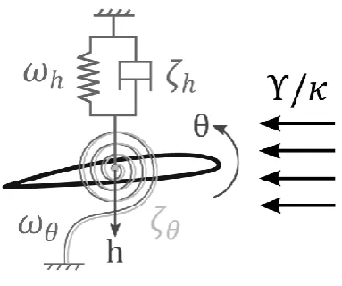
As an initial test system we consider an aerofoil with two degrees of freedom (plunge

ℎ

and twist

𝜃

).

Figure 1 shows a schematic of such a system, with dimensionless parameters as per Table 1 and the

airspeed parameter

Υ

; the airspeed per semichord. A frequency domain analysis of this system, under

Theodorsen’s unsteady aerodynamic theory yields a problem of the form:

((G

+ G

+ G

+ G

) 𝜒

− D

𝜒 − K

) 𝐱 = 𝟎,

(20)

where

𝐱 = [ℎ; 𝜃]

,

𝜅 = Υ 𝜒

⁄

is the reduced frequency, and

𝐶(𝜅)

is Theodorsen’s function, composed

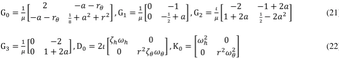
of a number of Bessel functions [4]. The matrix coefficients in Eq. 20 are:

G

=

[

2

−𝑎 − 𝑟

−𝑎 − 𝑟

+ 𝑎

+ 𝑟

] , G

=

[

0

−1

0 −

2

+ 𝑎] , G

=

[

_{1 + 2𝑎}

−2

−1 + 2𝑎

− 2𝑎

2

]

(21)

G

=

[0

_{0 1 + 2𝑎}

−2

] , D

= 2𝜄 [

𝜁

₀

𝜔

_𝑟

_𝜁

0

𝜃

𝜔

] , K

= [

𝜔

0

0

𝑟

_𝜔

2

]

(22)

with parameters as per Table 1. See Pons and Gutschmidt [28] or Hodges and Pierce [4] for details.

Taking

𝐶(𝜅) = 1

corresponds to the assumption of quasisteady aerodynamics, and with a change of

variables produces a polynomial system:

where

Υ = 𝑈 𝑏

⁄

is the local airspeed per semichord. This polynomial system be linearized and solved

with the operator determinant method of Section 3.

Figure 1.

Schematic of section model

Table 1: Parameter values for the section model

Parameter

Value

mass ratio –

𝜇

20

radius of gyration –

𝑟

0.4899

bending nat. freq. –

𝜔

0.5642 rad/s

torsional nat. freq. –

𝜔

1.4105 rad/s

bending damping –

𝜁

1.4105 %

torsional damping –

𝜁

2.3508 %

static imbalance –

𝑟

−0.1

pivot point location –

𝑎

−0.2

The results of this process are shown in Figure 2(a), which includes a contour plot of the system.

The flutter point is located at

𝜒 = 1.20 rad/s

and

Υ = 1.98 Hz

(

𝜅 = 0.606

). This agrees with

nondimensional analytical results by Hodges and Pierce [4]. We can, however, go further than an

analytical approach: we increase the matrix coefficient system size arbitrarily (and the polynomial

system order) and still obtain exact solutions. A direct solver for polynomial flutter problems of

arbitrary size and order has never before been presented.

We can also consider the case when

𝐶(𝜅)

is fully variable. The resulting MEP is nonlinear;

however a variety of approximations for Theodorsen’s function are available. We take a rational

function given by Jones [36]:

𝐶(𝜅) =

with

𝑐

= −0.2808𝜄

,

𝑐

= −0.01365

,

𝑐

= −0.3455𝜄.

Manipulating Eq. 20 we then obtain a

polynomial problem of maximum order

𝜅

𝜒

, requiring a custom linearization of

10

blocks width.

This be solved via the operator determinant method in under 0.2s on a laptop computer. The results

are shown in Figure 2(b), also with a contour plot of the system. The fact that this solver is direct is a

significant advantage over existing solvers for systems of this form.

Figure 2.

Flutter point results for the section model with two aerodynamic models.

5.2.

Goland wing

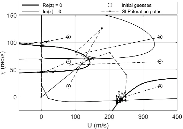
As a benchmark test for our iterative algorithms, we analyse the well-known Goland Wing test

case – representing a cantilever Euler-Bernoulli beam and Saint-Venant torsion model, with strip

theory Theodorsen aerodynamics [37]. Originally a differential MEP (containing spatial derivatives as

well as eigenvalue parameters), it is transformed by the Generalised Laplace Transform Method

(GLTM) [35] into a nonlinear algebraic problem or fixed size (

12 × 12

). This transformation is

without discretisation error, though it comes at the cost of obscuring the internal structure of the

model – hence we treat the transformed problem as black-box nonlinear MEP. There is a small

variation in parameter values for the Goland wing and so we take parameter values from Pons and

Gutschmidt [35] and Wang [38]. For these parameters the Goland wing’s first flutter point is located

at airspeed

𝑈

= 138 m/s

and modal frequency

𝜒

= 69.9 rad/s

. The first divergence point (static

instability) is located nearby at

𝑈

= 253 m/s

. Figure 3 shows example SLP iteration paths

literature. Figure 4 shows the convergence basins of the SLP and ICP algorithms to the flutter point,

computed numerically. The SLP algorithm has the larger basin; though both are very satisfactory and

the ICP is more computationally efficient.. The SLP algorithm is likely to be attractive for smaller

systems with little a priori knowledge, whereas the ICP is effective for larger and more expensive

systems, for which an initial flutter point estimate from an approximate model be available.

Figure 3.

Six example iterations of the SLP algorithms applied to the Goland wing.

6.

Conclusions

In this paper we have demonstrated and discussed the use of multiparameter solution techniques

for the solution of aeroelastic stability problems. We have introduced the link between multiparameter

spectral theory and stability analysis, and we showed how this link can be used to reformulate

stability problems with a complex-valued stability metric and a pertinent environmental parameter

into a two-parameter eigenvalue problem. We demonstrated that this allows the direct solution of

polynomial stability problems, as well as approximate direct and iterative solution methods for

strongly nonlinear problems. The application of multiparameter methods – in aeroelasticity and in

other disciplines – has the potential to provide a wide variety of new methods for stability analysis.

References

[1]

Dowell, E. H.,

Aeroelasticity of plates and shells

, Noordhoff International Publishing, Leyden,

The Netherlands, 1975.

[2]

Dowell, E. H., and Ilgamov, M.,

Studies in Nonlinear Aeroelasticity

, Springer-Verlag, New

York, 1988.

[3]

Bisplinghoff, R. L., Ashley, H., and Halfman, R. L.,

Aeroelasticity

, Addison-Wesley, Reading,

MA, 1957.

[4]

Hodges, D. H., and Pierce, G. A.,

Introduction to Structural Dynamics and Aeroelasticity

,

Cambridge University Press, New York, 2011.

[5]

Hassig, H. J., “An approximate true damping solution of the flutter equation by determinant

iteration.,”

Journal of Aircraft

, 8, 11 (1971), pp. 885–889. DOI:10.2514/3.44311.

[6]

Haddadpour, H., and Firouz-Abadi, R. D., “True damping and frequency prediction for

aeroelastic systems: The PP method,”

Journal of Fluids and Structures

, 25, 7 (2009), pp.

1177–1188. DOI:10.1016/j.jfluidstructs.2009.06.006.

[7]

Namini, A., Albrecht, P., and Bosch, H., “Finite element-based flutter analysis of

cable-suspended bridges,”

Journal of Structural Engineering

, 118, 6 (1992), pp. 1509–1526.

DOI:10.1061/(ASCE)0733-9445(1992)118:6(1509).

[8]

Chen, P. C., “Damping perturbation method for flutter solution: the g-method,”

AIAA Journal

,

38, 9 (2000), pp. 1519–1524. DOI:10.2514/2.1171.

[9]

Lind, R., and Brenner, M.,

Robust aeroservoelastic stability analysis

, Springer-Verlag,

London, 1999.

[10] Borglund, D., “Robust aeroelastic stability analysis considering frequency-domain

aerodynamic uncertainty,”

Journal

of

Aircraft

,

40,

1

(2003),

pp.

189–193.

DOI:10.2514/2.3074.

[11] Borglund, D., “The mu-k method for robust flutter solutions,”

Journal of Aircraft

, 41, 5

(2004), pp. 1209–1216. DOI:10.2514/1.3062.

[13] Afolabi, D., “Flutter analysis using transversality theory,”

Acta mechanica

, 103, 1–4 (1994),

pp. 1–15. DOI:10.1007/BF01180214.

[14] Afolabi, D., Pidaparti, R. M. V., and Yang, H. T. Y., “Flutter Prediction Using an Eigenvector

Orientation Approach,”

AIAA Journal

, 36, 1 (1998), pp. 69–74. DOI:10.2514/2.353.

[15] Meerbergen, K., Schröder, C., and Voss, H., “A Jacobi-Davidson method for

two-real-parameter nonlinear eigenvalue problems arising from delay-differential equations,”

Numerical

Linear

Algebra

with

Applications

,

20,

5

(2013),

pp.

852–868.

DOI:10.1002/nla.1848.

[16] Meerbergen, K., and Spence, A., “Inverse Iteration for Purely Imaginary Eigenvalues with

Application to the Detection of Hopf Bifurcations in Large-Scale Problems,”

SIAM Journal on

Matrix Analysis and Applications

, 31, 4 (2010), pp. 1982–1999. DOI:10.1137/080742890.

[17] Hochstenbach, M. E., and Plestenjak, B., “A Jacobi-Davidson Type Method for a Right

Definite Two-Parameter Eigenvalue Problem,”

SIAM Journal on Matrix Analysis and

Applications

, 24, 2 (2002), pp. 392–410. DOI:10.1137/S0895479801395264.

[18] Hochstenbach, M. E., Muhič, A., and Plestenjak, B., “On linearizations of the quadratic

two-parameter eigenvalue problem,”

Linear Algebra and its Applications

, 436, 8 (2012), pp. 2725–

2743. DOI:10.1016/j.laa.2011.07.026.

[19] Plestenjak, B., “A continuation method for a weakly elliptic two-parameter eigenvalue

problem,”

IMA Journal of Numerical Analysis

, 21, 1 (2001), pp. 199–216.

DOI:10.1093/imanum/21.1.199.

[20] Quarteroni, A., Sacco, R., and Saleri, F.,

Numerical mathematics

, Springer-Verlag Berlin,

Berlin, Germany, 2007.

[21] Cottin, N., “Dynamic model updating – a multiparameter eigenvalue problem,”

Mechanical

Systems and Signal Processing

, 15, 4 (2001), pp. 649–665. DOI:10.1006/mssp.2000.1362.

[22] Hochstenbach, M. E., Muhič, A., and Plestenjak, B., “Jacobi–Davidson methods for

polynomial two-parameter eigenvalue problems,”

Journal of Computational and Applied

Mathematics

, 288 (2015), pp. 251–263. DOI:10.1016/j.cam.2015.04.019.

[23] Meerbergen, K., and Plestenjak, B., “A Sylvester-Arnoldi type method for the generalized

eigenvalue problem with two-by-two operator determinants,”

Numerical Linear Algebra with

Applications

, 22, 6 (2015), pp. 1131–1146. DOI:10.1002/nla.2005.

[24] Hochstenbach, M. E., and Plestenjak, B., “Harmonic Rayleigh–Ritz extraction for the

multiparameter eigenvalue problem,”

Electronic Transactions on Numerical Analysis

, 29

(2008), pp. 81–96.

[25] Muhič, A., and Plestenjak, B., “On the quadratic two-parameter eigenvalue problem and its

linearization,”

Linear Algebra and its Applications

, 432, 10 (2010), pp. 2529–2542.

DOI:10.1016/j.laa.2009.12.022.

[26] Muhič, A., and Plestenjak, B., “On the singular two-parameter eigenvalue problem,”

Electronic Journal of Linear Algebra

, 18 (2009), pp. 420–437.

[27] Plestenjak, B., and Muhič, A.,

MultiParEig 1.0

, MATLAB File Exchange, Ljubljana,

Slovenia, 2015.

[29] Ruhe, A., “Algorithms for the Nonlinear Eigenvalue Problem,”

SIAM Journal on Numerical

Analysis

, 10, 4 (1973), pp. 674–689. DOI:10.1137/0710059.

[30] Pons, A., “Aeroelastic flutter as a multiparameter eigenvalue problem,” Master’s Thesis,

University of Canterbury, 2015, Gutschmidt, S.

[31] Plestenjak, B., “Numerical methods for nonlinear two-parameter eigenvalue problems,”

BIT

Numerical Mathematics

, 56, 1 (2016), pp. 241–262. DOI:10.1007/s10543-015-0566-9.

[32] Podlevskyi, B. M., “Numerical solution of some two-parameter eigenvalue problems,”

Journal

of Mathematical Sciences

, 165, 2 (2010), pp. 214–220. DOI:10.1007/s10958-010-9791-6.

[33] Podlevskii, B. M., “Newton’s method as a tool for finding the eigenvalues of certain

two-parameter (multitwo-parameter) spectral problems,”

Computational

Mathematics

and

Mathematical Physics

, 48, 12 (2008), pp. 2140–2145. DOI:10.1134/S0965542508120038.

[34] Golub, G. H., and Van Loan, C. F.,

Matrix computations

, The Johns Hopkins University Press,

Baltimore, MA, 2013.

[35] Pons, A., and Gutschmidt, S., “Aeroelastic Flutter of Continuous Systems: A Generalized

Laplace Transform Method,”

Journal of Applied Mechanics

, 83, 8, (2016), p. 081005.

DOI:10.1115/1.4033597.

[36] Jones, R.,

Operational treatment of the nonuniform-lift theory in airplane dynamics

, National

Advisory Committee for Aeronautics, Washington D.C., 1938.

[37] Goland, M., “The Flutter of a Uniform Cantilever Wing,”

Journal of Applied Mechanics

, 12, 4

(1945), pp. A197–A208.

[38] Wang, I., “Component Modal Analysis of a Folding Wing,” Master’s Thesis, Duke University,

2011, Dowell, E.

Arion Pons, M.E. (Ph.D. student): Department of Engineering, University of Cambridge,

Trumpington st., Cambridge CB2 1PZ, United Kingdom (

[email protected]

). The author gave a

presentation of this paper during one of the conference sessions.

Stefanie Gutschmidt, Senior Lecturer: Department of Mechanical Engineering, University of

Canterbury, Private Bag 4800, Christchurch 8140, New Zealand