Magneto Hydrodynamic Orthogonal Stagnation Point Flow of a Power Law Fluid Toward a Stretching Surface

Magneto Hydrodynamic Orthogonal Stagnation Point

Flow of a Power-Law Fluid toward a Stretching Surface

Manisha Patel1, Munir Timol2 1

Department of Mathematics, Sarvajanik College of Engineering & Technology, Surat, India 2

Department of Mathematics, Veer Narmad South Gujarat University, Surat, India E-mail: {manishapramitpatel, mgtimol}@gmail.com

Received April 27, 2011; revised May 25, 2011; accepted June 5, 2011

Abstract:

Steady two dimensional MHD stagnation point flow of a power law fluid over a stretching surface is inves-tigated when the surface is stretched in its own plane with a velocity proportional to the distance from the stagnation point. The fluid impinges on the surface is considered orthogonally. Numerical and

analytical

solutions are obtained for different cases.

Keywords: Stagnation Point Flow, Galerkin’s, Finite Difference Method, Stretching Surface.

1. Introduction

The stagnation point is a point on the surface of a body submerged in a fluid flow where the fluid velocity is zero. Stagnation flow, describing the fluid motion near the stagnation region, exists on all solid bodies moving in a fluid. The stagnation region encounters the highest pres-sure, the highest heat transfer, and the highest rates of mass deposition. The study of flow over a stretching sur-face has generated much interest in recent years in view of its numerous industrial applications such as extrusion of polymer sheets, continuous stretching, rolling and manufacturing plastic films and artificial fibers. The flow near a stagnation point has attracted many investigations during the past several decades because of its wide ap-plications such as cooling of electronic devices by fans, cooling of nuclear reactors, and many hydrodynamic processes [1-5].

The two-dimensional flow of a fluid near a stagnation point was first examined by Hiemenz [6], who demon-strated that the Navier-Stokes equations governing the flow can be reduced to an ordinary differential equation of third order using similarity transformation. Later the problem of stagnation point flow was extended in nu-merous ways to include various physical effects. The results of these studies are of great technical importance, for example in the prediction of skin-friction as well as heat/mass transfer near stagnation regions of bodies in high speed flows and also in the design of thrust bearings and radial diffusers, drag reduction, transpiration cooling

behaviors.

Chiam [12] and Mahapatra and Gupta [13] have inves-tigated the steady two-dimensional stagnation point flow of an incompressible viscous fluid over a flat deformable sheet when the sheet is stretched in its own plane with a velocity proportional to the distance from the stagnation point. It is shown that a boundary layer is formed near the stretching surface and that the structure of this boun-dary layer depends on the ratio of the velocity of the stretching surface to that of the frictionless potential flow in the neighborhood of the stagnation point. Recently, Patel et al. [5] have discussed the numerical solution for steady two-dimensional MHD forward stagnation point flow introducing the Crocco’s independent variable with Galerkin’s. In stagnation point flow, a rigid wall or a stretching surface occupies the entire horizontal x-axis, the fluid domain is y0 and the flow impinges on the wall either orthogonal or at an arbitrary angle of inci-dence.

In this paper we investigate steady two dimensional stagnation point flow of a power law fluid over a stret-ching surface, when the surface is stretched in its own plane with a velocity proportional to the distance from the stagnation point. The fluid impinges on the surface is considered orthogonally. Numerical and analytical solu-tions are obtained for different flow geometries along with graphical presentation.

2. Flow Analysis

The well-known Ostwald-de-Wale model of power-law fluid is purely phenomenological; however, it is useful in that approximately describes a great number of real non-Newtonian fluids. This model behaves properly un-der tensor deformation. Use of this model alone assumes that the fluid is purely viscous. Mathematically it can be represented in the form

1 2

1 : 2

n m





 

 

 _   _

 

 

(1)

where m and n are called the consistency and flow behavior indices respectively. If n1, the fluid is called pseudo plastic power law fluid and if n1, it is called dilatants power law fluid since the apparent viscosity decreases or increases with the increase shear of rate ac-cording as n1 or n1, if n1 the fluid will be Newtonian.

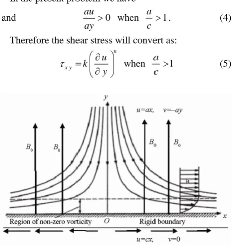
Consider the steady two-dimensional stagnation-point flow of power-law fluid flowing towards a flat surface coinciding with the plane y0, the flow being con-fined to the region y0. Two equal and opposing forces are applied on the stretching surface along the

x-axis so that the surface is stretched keeping the origin fixed as shown in Figure 1. The MHD equations for steady two-dimensional stagnation-point flow in the boundary layer towards the stretching surface are, in the usual notation,

0

u v

x y

 _ _

  (2) 2

0

( )

xy

B

u u U

u v U u U

x y x y

 



   

    

    (3)

Here the magnetic Reynolds number is assumed to be very small so that the induced magnetic field is neglected. Here u and v are the velocity components along the x and y direction, respectively. Further xy is stress tensor in

the direction of Y-axis perpendicular to X-axis. U x( ) stands for the stagnation-point velocity in the inviscid free stream. The stress tensor is defined by Equation (1).

In the present problem we have

and au 0

ay  when 1 a

c . (4) Therefore the shear stress will convert as:

n

x y

u k

y

 _{ } _



  when 1 a

[image:2.595.308.539.292.536.2]

c  (5)

Figure 1. A sketch of the physical problem.

[image:2.595.308.540.562.696.2]

[image:3.595.59.539.39.724.2]

Table 1.

n So0 So0.5 So1.0 So1.5 So2.0

0.4 0.1123 0.1252 0.1445 0.1564 0.1601 0.8 0.1512 0.1668 0.1748 0.1799 0.1869 1.2 0.1924 0.2214 0.2356 0.2455 0.2662 1.5 0.2358 0.2514 0.2636 0.2741 0.2852 2.0 0.2897 0.2999 0.3121 0.3255 0.3412

Table 2.

n So0 0.5So 1.0So 1.5So 2.0So

0.4 1.2216 1.3625 1.4886 1.6289 1.7865

0.8 1.0023 1.0423 1.0858 1.1821 1.3226

1.2 0.8984 0.9672 1.0115 1.1000 1.2101

1.5 0.8864 0.9355 1.0021 1.0552 1.1001

2.0 0.8876 0.9301 0.9864 0.9945 1.0477

Table 3.

n So0 0.5So 1.0So 1.5So 2.0So

[image:3.595.54.288.84.339.2]

0.4 3.8771 4.1332 4.4755 4.8163 5.2445 0.8 2.3854 2.5446 2.5845 2.8354 2.8714 1.2 1.9328 1.9454 2.0023 2.1426 2.1735 1.5 1.7001 1.7537 1.8817 1.9583 1.9966 2.0 1.5481 1.5841 1.6120 1.6526 1.6998

Table 4. Results of finite difference method of Case-I.

No. of iteration So0 0.5So So1.0 1.5So So2.0

1 1.02326 1.2326 1.2326 1.2326 1.2326

2 1.1688 1.3593 1.5393 1.7882 1.8385

3 1.1743 1.3637 1.5407 1.7890 1.8339

4 1.1715 1.3618 1.5392 1.7662 1.8328

5 1.1717 1.3621 1.5394 1.7914 1.8330

6 1.1717 1.3620 1.5394 1.7914 1.8330

Now the momentum Equation (3) become, in non-di-

mensional form, when a 1 c

2 0 _{( )}

n B

u u U K u

u v U u U

x y x y y



 

 

    

   _{ }  

    _ _ (6)

The boundary conditions are:

, 0 y 0

ucx v at  (7)

( ) , , y

uU x ax v ay at   (8)

where a and c are positive constants. Introducing stream function ( , )x Y , where

u y



 

 and =v x

  

 (9)

Following Labropulu [3], we assume that

( )

cxF y

  (10) Using Equations (9) and (10) into the Equation (6), we obtained





1 2

( ) ( ) ( ) ( )

1

n n

n F y F y F y F y

n

  

  _{ } 



 

2 2

2

( ) o ( ) o 0

a a F y S F y S

c c

 

     (11)

with the boundary conditions:

(0) 0

F  , F(0)1, F( ) a

c

   (12)

where

2 0

o

B S

c

 

 is the magnetic parameter.

Case-I: Newtonian fluid: consider n1 and /a c1 Equation (11) is converted in the following equation

2

( ) ( ) ( ) ( ) _o ( ) _o 1 0

F y  F y F y F y S F y S   (13)

with the boundary conditions:

(0) 0

F  , F(0)1, F( ) a c

   (14)

Case-II: if we consider case for n1, and let U0

(i.e. a0) then the Equation (11) is converted in 2

( ) ( ) ( ) ( ) _o ( ) 0

F y F y F y F y S F y  (15)

Subject to the boundary conditions;

(0) 0, (0) 1, ( ) 0

F  F  F  (16)

[image:3.595.56.284.365.437.2]

It is interesting to note that the above BVP Equation (15) has a simple analytic solution of the form

Figure 3. Variation of F(0) with S_o for a / c= 1.5.

[image:3.595.56.539.374.718.2]

[image:4.595.54.293.68.455.2]

Figure 5. Variation of F(0) with So for a / c= 1 ,

= 1

n .

Figure 6. Variation of F y with y( ) .

1

( ) [1 exp( )]

F y py

p

  

(17)

where 1/ 2

0

(1 )

p S

Method of solution: The transformed momentum Equation (11) is solved using Galerkin’s method after introducing Crocco’s variables [5,14]. The equation for Case-I (Equation (13)) is solved by T. Y. Na [8] using Finite difference method the graphical presentation of those tabular values (Table 3) is shown in Figure2. And the equation of Case-II (Equation (15)) is solved analyti-cally.

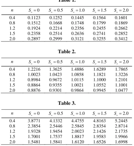
Results and discussion: The computed variation of

 

0

F with So and n is summarized in Tables1 and 2

for a c/ 1.1, 1.5 and 2.0, respectively. It can be con-clude (from the above Tables 1-3, Figures 2-4) that for a fixed value of So, F

 

0 increases with increase in n

in a small neighbourhood of a c/ 1 then it decreases for other values of a/c. From Tables 1-3, it is clear that for a fixed value of n and a c/ , the value of F

 

0 de-creases with increase in So. This behaviour may perhaps

be attributed to the change in the character of the flow as

It is interesting to note that when the velocity of the stretching surface is equal to the velocity of the inviscid stream



ac



, Equation (16) admit to the exact analytic solution F y( ) y. From this we can infer that when

ac, the velocity distribution near the stretching sur-face is the same as athat of a flow away from the sursur-face so that no boundary layer is formed near the surface. It should be mentioned here that when , the flow is not fric-tionless in a strict sense. In fact in this case the friction is uniformly distributed and does not, therefore, affect the motion.

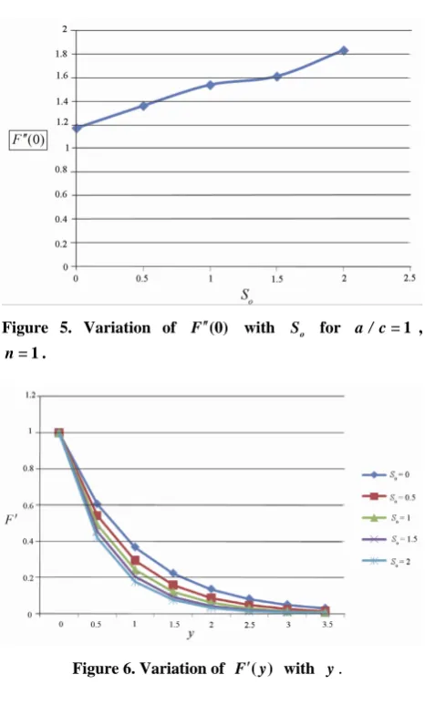
If we consider n1 then the entire flow geometry is reduced in Newtonian fluid, which is discussed as a Case-I with ac (i.e. a c/ 1, Table 4, Figure 5). For that case F

 

0 increases with increase in the val-ue of So for a fixed value of n1. If we consider

stream velocity is zero



n1



then the flow is treated as a uniform stagnation point flow, in this case F

 

y decreases with increase in y for a fixed value of So.

The graphical representation is shown in Figure 6.

3. References

[1] H. A. Attai, “Stagnation Point Flow towards a Stretching Surface through a Porous Medium with Heat Generation,”

Turkish Journal of Engineering & Environmental Scien- ces, Vol. 30, No. 5, 2006, pp. 299-306.

[2] F. M. Hayd and I. A. Hassanien, “Magnetohydrodynamic and Constant Suction/Injection Effects of Axisymmetric Stagnation Point Flow and Mass Transfer for Power-Law Fluids,”Indian Journal of Pure and Applied Mathematics, Vol. 17, No. 1, 1986, pp. 108-120.

[3] F. Labropulu and D. Li, “Stagnation Point Flow of a Second-Grade Fluid with Slip,” International Journal of Non-Linear Mechanics, Vol. 43, No. 9, 2008, pp. 941-947.

doi:10.1016/j.ijnonlinmec.2008.07.004

[4] B. Norfifah and I. Anuar, “MHD Stagnation-Point Flow of a Micropolar Fluid with Prescribed Wall Heat Flux,”

European Journal of Scientific Research, Vol. 35 No. 3, 2009, pp. 436-443.

[5] M. Patel and M. G. Timol, “Numerical Solution of Steady Two-Dimensional MHD forward Stagnation Point Flow,”

Applied Mathematical Science, Vol. 3, No. 4, 2009, pp. 187-193.

[6] K. Hiemenz, “Die Grenzschicht an Einem in Den Gleich-formingen Flussigkeitsstrom Eingetauchten Graden Krei- szylinder,” Dingler’s Polytechnic Journal, Vol. 326, 1911, pp. 321-324.

[7] F. Homann, “Der Einfluss Grosser Zahigkeit bei der Stromung um den Zylinder und um die Kugel,” Journal of Applied Mathematics and Mechanics/Zeitschrift für Angewandte Mathematik und Mechani, Vol. 16, No. 3, 1936, pp. 153-164.doi:10.1002/zamm.19360160304

[9] P. D. Ariel, “Hiemenz Flow in Hydromagnetics,” Acta Mechanica, Vol. 103, No. 1-4, 1994, pp. 31-43.

[10] K. R. Rajagopal, T. Y. Na and A. S. Gupta, “A Non Sim-ilar Boundary Layer on a Stretching Sheet in a Non-Newtonian Fluid with Uniform Free Stream,” Jour-nal of Mathematical Physics, Vol. 21, No. 2, 1987, pp. 189-200.

[11] K. R. Rajagopal, T. Y. Na and A. S. Gupta, “Flow of a Viscoelastic Fluid over a Stretching Sheet,” Rheologica Acta, Vol. 23, No. 2, 1984, pp. 213-215.

doi:10.1007/BF01332078

[12] T. C. Chiam, “Stagnation-Point Flow towards a

Stretch-ing Plate,” Journal of the Physical Society of Japan, Vol. 63, No. 6, 1994, pp. 2443-2444.

doi:10.1143/JPSJ.63.2443

[13] T. R. Mahapatra and A. S. Gupta, “Heat Transfer in Stagnation-Point Flow towards a Stretching Sheet,” Heat Mass Transfer, Vol. 38, No. 6, 2002, pp. 517-521. doi:10.1007/s002310100215

[14] T. C. Chiam, “Solution for the Flow of a Conducting Power-Law Fluid in a Transverse Magnetic Field and with a Pressure Gradient Using Crocco Variables,” Acta Mechanica, Vol. 137, No. 3-4, 1999, pp. 225-235.

Nomenclature:

u, v – velocity components in X, Y directions respec-tively

U – main stream velocity in X direction a, c – positive constants

_,, ij – usual shear stress tensor

_, e_ij – usual rate of deformation tensor/ Strain rate component

yx

 – stress tensor in the direction of X-axis perpen-dicular to Y-axis.

K – kinematic Viscosity

m – Physical constant n – flow behavior indices

0

B – Imposed magnetic field MHD – Magneto hydro dynamics

 – field density

 – Electrical conductivity

p

C – Specific heat

 – Stream function F – Similarity function

o

S – Magnetic parameter – 2 0 B