Measuring Dynamic Correlations of Words in Written Texts with an Autocorrelation Function

http://www.scirp.org/journal/jdaip ISSN Online: 2327-7203

ISSN Print: 2327-7211

DOI: 10.4236/jdaip.2019.72004 May 27, 2019 46 Journal of Data Analysis and Information Processing

Measuring Dynamic Correlations of Words in

Written Texts with an Autocorrelation Function

Hiroshi Ogura, Hiromi Amano, Masato Kondo

Department of Information Science, Faculty of Arts and Sciences, Showa University, Fujiyoshida City, Yamanashi, Japan

Abstract

In this study, we regard written texts as time series data and try to investigate dynamic correlations of word occurrences by utilizing an autocorrelation function (ACF). After defining appropriate formula for the ACF that is suita-ble for expressing the dynamic correlations of words, we use the formula to calculate ACFs for frequent words in 12 books. The ACFs obtained can be classified into two groups: One group of ACFs shows dynamic correlations, with these ACFs well described by a modified Kohlrausch-Williams-Watts (KWW) function; the other group of ACFs shows no correlations, with these ACFs fitted by a simple stepdown function. A word having the former ACF is called a Type-I word and a word with the latter ACF is called a Type-II word. It is also shown that the ACFs of Type-II words can be derived theoretically by assuming that the stochastic process governing word occurrence is a ho-mogeneous Poisson point process. Based on the fitting of the ACFs by KWW and stepdown functions, we propose a measure of word importance which expresses the extent to which a word is important in a particular text. The va-lidity of the measure is confirmed by using the Kleinburg’s burst detection algorithm.

Keywords

Autocorrelation Function, Word Occurrence, Kohlrausch-Williams-Watts Function, Stochastic Process, Poisson Point Process

1. Introduction

We use language to convey our ideas. Since our physical function is limited to speaking or writing only one word at a time, we must transform our complex ideas into linear strings of words. In this transformation, it is essential to use memory, because our thought processes are far more complex than a linear object, and this How to cite this paper: Ogura, H., Amano,

H. and Kondo, M. (2019) Measuring Dy-namic Correlations of Words in Written Texts with an Autocorrelation Function. Journal of Data Analysis and Information Processing, 7, 46-73.

https://doi.org/10.4236/jdaip.2019.72004

Received: March 14, 2019 Accepted: May 24, 2019 Published: May 27, 2019

Copyright © 2019 by author(s) and Scientific Research Publishing Inc. This work is licensed under the Creative Commons Attribution International License (CC BY 4.0).

DOI: 10.4236/jdaip.2019.72004 47 Journal of Data Analysis and Information Processing one-dimensional is the origin of various types of correlations observed in written texts or speeches. In this regard, the questions that arise are how to characterize various types of correlations in linguistic data and how to relate them to our thought processes. These questions motivated us to initiate the study of dynamic correlations in written texts.

One major way to capture the correlations is to analyze word co-occurrence statistics, which is a traditional quantitative method in linguistics. This approach has been successfully applied to the extraction of semantic representations [1], automatic key word and key phrase extraction [2] [3], local or global context analysis [4], measuring similarities at the word or context level [5], and many other tasks. Another way to investigate correlations in linguistic data is to use a mapping scheme, that is, to translate the given sequence of words or characters in a text into a time series and thereby capture the correlations in a dynamical framework. The mapping scheme has an obvious advantage for our purpose be-cause dynamic correlations can be related to the underlying stochastic processes that generate the time-series data. This means that if we successfully model the translated time-series data by a certain type of stochastic process, then we can obtain insights from that model to understand relations between the text and the complex idea represented. Up to now, time-series analyses of written texts have been made at three different linguistic levels: Mappings performed at the letter level [6] [7] [8], at the word level [9] [10] [11], and at the context or topic level

[12] [13]. Among these, word-level mapping is attractive because the funda-mental minimum unit of thought is considered to exist at the word level [10]. Furthermore, word-level mapping offers a simple procedure by which a given sequence of words is converted into a time series without any additional mani-pulations. In the mapping, all the words are enumerated in order of appearance, as i=1, 2,,N, where i plays the role of time in a text having a total of N words. This means that the time unit of the word-level mapping is selected as one word, and therefore the conversion is simply equivalent to assigning a unique index i to each word according to the order of its appearance in a text. Hereafter, we call this index the “word-numbering time”. Studies using word-level mapping share, however, the common disadvantage that the dynamic correlations cannot be ex-pressed in an appropriate way, and so such mapping is not suitable for discuss-ing the stochastic properties of each word. The major reason for this is that we cannot define an autocorrelation function (ACF) appropriately when we use the word-numbering time, as will be described in Section 3. This situation necessi-tates the use of gap-distribution functions [9] [11] or more sophisticated ap-proaches [10] to characterize stochastic properties of words when we apply the word-numbering time. The utilization of ACFs is, however, essential in this study because it is the most direct quantity for expressing dynamic correlations of words, and thus it will be of great help in relating dynamic correlations with underlying stochastic processes.

DOI: 10.4236/jdaip.2019.72004 48 Journal of Data Analysis and Information Processing With that modification, we then calculate ACFs for words in written texts and investigate word-level dynamic correlations in terms of the functional forms of the ACFs. In particular, we focus on dynamic correlations ranging from a few sentences to several tens of sentences because complex ideas require such a length to be conveyed. Through the analysis of ACFs, we will find that the func-tional form of ACFs for words with dynamic correlations are completely different from those without dynamic correlations. Using this result as a base, a measure that quantifies the strength of dynamic correlations will be presented, and the validity of the measure will be discussed. The measure expresses, in a sense, how important the corresponding word is in a text and thus has a wide range of real applications in which the importance of each word is required.

The rest of the paper is organized as follows. In the next section, we outline related studies with special emphasis on how the models used in the related stu-dies can be interpreted in terms of stochastic processes. Then, we devote a sec-tion to explaining the modificasec-tion of the word-level mapping, the definisec-tion of an appropriate ACF for word occurrences, and how to calculate the ACF from real written texts. Section 4 describes 12 texts, frequent words from which are in-vestigated using ACFs. These 12 texts represent a wide variety of written linguistic data. Section 5 shows our systematic analysis of ACFs calculated for words in the 12 texts. A measure representing word importance in terms of dynamic correla-tions is also presented. In the final section, we give our conclusions and suggest directions for future research.

2. Related Work

2.1. Models of Word Occurrences

A homogeneous Poisson point process [14] with word-numbering time can be considered as the simplest model of word occurrences in texts, because it has the key property of “complete independence” in which the number of word occur-rences of a considered word in each bounded sub-region in “time” along text will be completely independent to all the others. The homogeneous Poisson point process is suitable if a word occurs with a very low constant probability for each unit time. This means that the probability of word occurrence per unit time (per each word) must be stationary and fixed at a certain low value throughout a text in order to apply the homogeneous Poisson point process appropriately. This stationary condition is too strong and limits the applicability of the model to word occurrences in real texts. Therefore, extensions of the homogeneous Poisson point process have been tried to remove the limitation. We briefly de-scribe here how word occurrences have been modeled in two related studies in which the extensions of the homogeneous Poisson process can be achieved.

oc-DOI: 10.4236/jdaip.2019.72004 49 Journal of Data Analysis and Information Processing currence rate. The model does not explicitly capture the dynamic correlations of a considered word, but, instead, simply indicates the time interval where the dy-namic correlations persist as the duration of the excited state.

A further extension has been achieved by use of an inhomogeneous Poisson process which is defined as a Poisson point process having a time-varying oc-currence rate [15] [16]. Adilson et al. [9] have adopted the formulation of one of the inhomogeneous Poisson processes, i.e., the Weibull process [14] [16] [17], for modeling word occurrences in texts.

Obviously, the two models mentioned above have more expressive power than that of a homogeneous Poisson process. However, these models do not serve to clarify dynamic correlations of word occurrences because the key property of “complete independence” is also common to these two models. In other words, since the “complete independence” property is inherited to these two models, an occurrence of a considered word in a text does not affect the probability of occur-rences of the word at different times. This memoryless property makes the appli-cations of these models hard to clarify dynamic correlations of word occurrences.

Another unsatisfactory point which is common to the two related studies is that the gap distribution function has been used to characterize stochastic prop-erties of a considered word. Note that when the word-numbering time is em-ployed, the “gap” is merely the number of other words encountered between oc-currences of a considered word in the text. Therefore, that distribution function does not express the dynamical correlation explicitly, although it is suitable to present characteristics of stochastic processes such as homogeneous Poisson, mixture of two homogeneous Poisson and inhomogeneous Poisson processes in which the complete independence property is held.

To avoid the inappropriate use of the gap distribution function for representing dynamic correlations, we will discard the gap distribution function and in the next section, we will introduce an ACF that is more suitable for analyzing dy-namic correlations of words.

2.2. Models of Linguistic Data with ACFs

There are other works in which linguistic data are treated as time series, as they are in this work and in which some methods of time series analysis are used to achieve the researchers’ purposes. Examples of classical works that use ACFs can be seen in [18] and [19], where time series of sentence length were analyzed with ACFs. A more generalized method for applying time-series analysis to linguistic data has been established by Pawlowski [20]. He used ACFs for analyzing se-quential structures in text at phonetic and phonological levels [20] [21] [22] [23]. That is, the direction of Pawlowski’s study is similar to ours, although he did not investigate dynamic correlations of word occurrences.

3. Calculation of ACF for Written Texts

DOI: 10.4236/jdaip.2019.72004 50 Journal of Data Analysis and Information Processing and analyze dynamic correlations in written texts. In standard signal processing theory, the definition of an ACF for a stationary system, C t

( )

[24], and its normalized expression, Φ

( )

t , are given by

( )

1 ₀

( ) (

)

lim T d

T

C t A A t

T τ τ τ

→∞ =

_∫

+ (1)

( )

_{( )}

( )

( ) (

)

( ) ( )

0 0 1 lim d 1

0 _{lim d}

T T

T T

A A t

C t _T

t

C _{A A}

T

τ τ τ

τ τ τ

→∞ →∞

+ Φ = =

∫

∫

(2)

where A

( )

τ is a time-varying signal of interest. As seen in the equations, the ACF measures the correlation of a signal A

( )

τ with a copy of itself shifted by some time delay t. A slightly different definition of an ACF for a random process is used in the area of time-series analysis [24] [25]. That definition is

( )

(

( )

)

(

2

(

)

)

,

E A A t

R t τ µ τ µ

σ

 − + − 

 

=

(3) where µ = E A t_

( )

_ and σ2=E_

(

A t

( )

−µ

)

2_ are the mean (the expectation value) and variance, respectively, of the stochastic signal A t

( )

. Assuming an ergodic system, in which the expectation can be replaced by the limit of a time average [24], Equations (2) and (3) are basically equivalent except that Equation (3) handles the deviation from the mean value and measures the correlation of the deviation but Equation (2) measures the dynamic correlation of A

( )

τ itself. This slight difference between Equations (2) and (3), however, affects the limit values of the ACFs as the lag t approaches infinity in a different manner:

( )

0

R t → as t→ ∞ always holds, from its definition, but limt→∞Φ

( )

t is not always zero. We adopt Equation (2) as the definition of ACF in this study, be-cause the limit value of ACF given by limt→∞Φ

( )

t carries important informa-tion about a considered word, as will be described in Subsecinforma-tion 5.5.

In order to calculate an ACF for a word based on Equation (2), we must de-fine both the meaning of A t

( )

for a word and the meaning of time t for a written text. Since we intend to clarify the dynamic properties of words through ACFs, it is natural to have A t

( )

indicating whether or not the considered word occurs at time t. Therefore, we define A t

( )

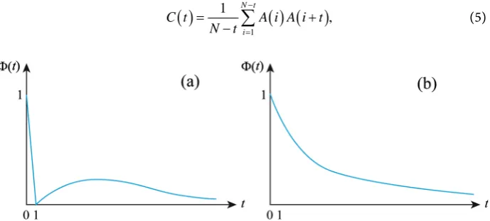
as a stochastic binary variable that takes value one if the word occurs at time t and otherwise takes value zero. Next, we consider an appropriate definition of the time unit such that the ACF calcu-lated by Equation (2) will have properties that are preferable for the analysis of the dynamic characteristics of word occurrences. As mentioned before, if we use the word-numbering time, then the ACF shows a curious behavior that greatly im-pairs the use of ACFs. The problem with using word-numbering time is that

( )

t

Φ _{with word-numbering time invariably takes the value zero at} t=1

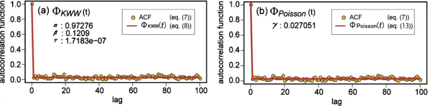
DOI: 10.4236/jdaip.2019.72004 51 Journal of Data Analysis and Information Processing shown in Figure 1(b). Acceptance of the curious behavior shown in Figure 1(a)

means that we discard almost all of the standard methods that have been devel-oped in various fields for analyzing ACFs. For example, analysis through curve fitting with model equations is widely used to characterize observed ACFs. Since the functional form of ACFs with the curious behavior seen in Figure 1(a) has not been identified, we must forgo this analysis when we use the word-numbering time. However, if an ACF behaves as it does in a usual linear system and shows gradual decrease of correlation, as seen in Figure 1(b), then a suitable model function can be used, as will be seen in Subsection 5.2.

Since the curious behavior seen in Figure 1(a) is unacceptable, we must in-troduce another definition of time unit, different from the word-numbering time. In this study, we use ordinal sentence number along a text as a time. Spe-cifically, if a considered word occurs in the t-th sentence (counting from the be-ginning of the text), then we say that the word occurs at time t. Hereafter, this definition of time will be called “sentence-numbering time”. We can verify that the sentence-numbering time is suitable for our purpose by the following reason-ing. Consider a word that plays a central role in the explanation of a certain idea. Then, in the context of describing the idea, the word is sequentially used over mul-tiple sentences after the first occurrence. This means that we can expect a higher probability of the word’s occurrence in a subsequent sentence given that the word occurred in the previous sentence; this makes the ACF take rather high values at

1

t= and gradually decrease as t increases, which is the natural behavior of ACFs seen in Figure 1(b). Therefore, the sentence-numbering time enables the ACF to behave as a normal monotonically decreasing function of time.

With the sentence-numbering time, we can define the signal of word occur-rence, A t

( )

, as a stochastic binary variable:

( )

1

₍

(

the word occurs in the -th sentence

)

₎

0 the word does not occur in the -th sentence

t A t

t

 = 

 (4)

where t is a non-negative integer. From Equation (1), we can define the discrete time analog of the continuous time ACF as

( )

( ) (

)

1

1

, N t

i

C t A i A i t

N t

−

=

= +

[image:6.595.196.541.540.696.2]

−

∑

(5)

DOI: 10.4236/jdaip.2019.72004 52 Journal of Data Analysis and Information Processing where N is the number of sentences in a considered text. A further simplification can be achieved by noting that A i

( )

is a binary variable. Let p_j be the ordinal sentence number at which the considered word occurs: that is, p1 is the

sen-tence number of the first occurrence of a considered word, p2 is that of the

second occurrence, and so on. If A i

( )

is zero in Equation (5), then the contri-bution of A i A i t

( ) ( )

+ in the equation is vanished. Thus, it is sufficient to think only about A p

( )

j , which is assumed to be 1, in Equation (5). Equation (5) then simplifies to

( )

{ }

( ) (

)

( ) (

)

(

)

1 1 1 1 1 , j N t i p m j j j m j j

C t A i A i t

N t

A p A p t N t

A p t N t − ∈ = = = + − = + − = + −

∑

∑

∑

(6)

where we have assumed that the total number of occurrences of the word in a text is m. The third equality holds because A p

( )

j =1 by the definition of pj. Substituting t=0 into the above equation yields C

( )

0 =m N, and this leads us to the normalized expression of the ACF:

( )

_{( )}

( )

₍

₎

(

)

1 . 0 m j j

C t N

t A p t

C m N t =

Φ = = +

−

∑

(7) Throughout this work, we use Equation (7) to calculate the normalized ACF of a word.

4. Texts

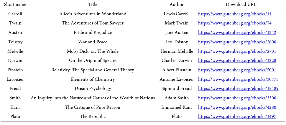
[image:7.595.55.540.517.729.2]

We used the English version of 12 books as written texts for this work. They are listed in Table 1 with their short names and some information. The books were

Table 1. Summary of English texts employed.

Short name Title Author Download URL

Carroll Alice’s Adventures in Wonderland Lewis Carroll https://www.gutenberg.org/ebooks/11

Twain The Adventures of Tom Sawyer Mark Twain https://www.gutenberg.org/ebooks/74

Austen Pride and Prejudice Jane Austen https://www.gutenberg.org/ebooks/1342

Tolstoy War and Peace Leo Tolstoy https://www.gutenberg.org/ebooks/2600

Melville Moby Dick; or, The Whale Herman Melville https://www.gutenberg.org/ebooks/2701

Darwin On the Origin of Species Charles Darwin https://www.gutenberg.org/ebooks/1228

Einstein Relativity: The Special and General Theory Albert Einstein https://www.gutenberg.org/ebooks/5001

Lavoisier Elements of Chemistry Antoine Lavoisier https://www.gutenberg.org/ebooks/30775

Freud Dream Psychology Sigmund Freud https://www.gutenberg.org/ebooks/15489

Smith An Inquiry into the Nature and Causes of the Wealth of Nations Adam Smith https://www.gutenberg.org/ebooks/3300

Kant The Critique of Pure Reason Immanuel Kant https://www.gutenberg.org/ebooks/4280

DOI: 10.4236/jdaip.2019.72004 53 Journal of Data Analysis and Information Processing obtained through Project Gutenberg (http://www.gutenberg.org). Five of them are popular novels (Carroll, Twain, Austen, Tolstoy, and Melville) and the rest are chosen from the categories of natural science (Darwin, Einstein, and La-voisier), psychology (Freud), political economy (Smith), and philosophy (Kant and Plato), so as to represent a wide range of written texts. The preface, contents and index pages were deleted before starting text pre-processing because they may act as noise and may affect the final results.

Before calculating the normalized ACF with Equation (7), we applied the fol-lowing pre-processing procedures to each of the texts.

1) Blank lines were removed and multiple adjacent blank characters were replaced with a single blank character.

2) Each of the texts was split into sentences using a sentence segmentation tool. The software is available from https://cogcomp.org/page/tools/.

3) Each uppercase letter was converted to lowercase.

4) Comparative and superlative forms of adjectives and adverbs were converted into positive forms. Plural forms of nouns were converted into singular ones and also all the verb forms except the base form were converted into their base form. For these conversions, we used Tree Tagger which is a language independent part-of-speech tagger available from

http://www.cis.uni-muenchen.de/~schmid/tools/TreeTagger/.

5) Strings containing numbers were deleted. All punctuation characters were replaced with a single blank character.

6) Stop-word removal was performed by use of the stop-word list built for the experimental SMART [26] information retrieval system.

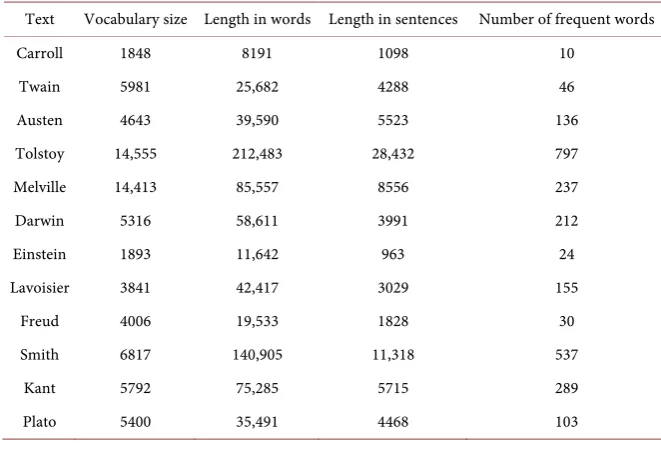
[image:8.595.205.536.505.737.2]

Some basic statistics of the used texts, evaluated after the pre-processing proce-dures, are listed in Table 2. The heading “frequent word” at the last column of the table indicates that words listed in the column appeared in at least 50 sentences

Table 2. Basic statistics of the 12 texts, evaluated after pre-processing procedures.

Text Vocabulary size Length in words Length in sentences Number of frequent words

Carroll 1848 8191 1098 10

Twain 5981 25,682 4288 46

Austen 4643 39,590 5523 136

Tolstoy 14,555 212,483 28,432 797

Melville 14,413 85,557 8556 237

Darwin 5316 58,611 3991 212

Einstein 1893 11,642 963 24

Lavoisier 3841 42,417 3029 155

Freud 4006 19,533 1828 30

Smith 6817 140,905 11,318 537

Kant 5792 75,285 5715 289

DOI: 10.4236/jdaip.2019.72004 54 Journal of Data Analysis and Information Processing in the relevant text. Note that the set of these frequent words for each text con-tains not only content words, some of which play central roles in the explanation of important and specific ideas in the text, but also words that occur frequently merely due to their functionality. The former are context-specific but the latter are not. In other words, the former are important to describe an idea and thus they are expected to be highly correlated with duration of, typically, several tens of sentences where the idea is described. On the other hand, the latter are not expected to show any correlations because their occurrences are not con-text-specific but are governed by chance. As will be described in the next section, we will calculate the normalized ACF with Equation (7) for the frequent words and will find how these two kinds of frequent words behave differently in terms of ACF. For the calculation, we mainly employed the R software environment for statistical computing (version 3.1.2) [27] to implement our algorithm, but supplementary coding in the Java programming language (JDK 1.6.0) was used to speed up the calculation.

5. Characteristics of Correlated and Non-Correlated ACFs

5.1. Typical Examples of Correlated and Non-Correlated ACFs

Figure 2 and Figure 3 show typical ACFs for words exhibiting strong dynamic correlations (Figure 2) and for those exhibiting no correlation (Figure 3). In these figures, words were picked from the frequent words of the Darwin text. As depicted in Figure 2, the ACF for a word having strong correlation takes the ini-tial value of Φ

( )

0 =1, then gradually decreases as the lag increases. Here the

“lag” simply means the parameter t of Φ

( )

t and is the distance between two different time points at which two values of A i

( )

are considered to calculate their correlation. The behaviors of ACFs in Figure 2 indicate that once a word emerges in a text, then it frequently appears in the following several tens of sen-tences but the probability of appearance gradually decreases. This situation can be thought as relaxations of the occurrence probability in a considered text and is very similar to various relaxation processes observed in real linear systems. The monotonically decreasing property, which is common to ACFs for linear systems, thus validates our definition of the time unit.

In contrast with these, each of the ACFs in Figure 3 takes the initial value of

( )

0 1

Φ = _{, then abruptly decreases at} t=1 to some constant value γ unique

to each ACF at t≥1. The stepdown behavior observed in Figure 3 indicates

that the duration of dynamic correlation is essentially zero for each of the words picked in Figure 3 and so these words do not have any dynamic correlations. 5.2. Curve Fitting Using Model Functions

[image:10.595.124.541.67.269.2]

DOI: 10.4236/jdaip.2019.72004 55 Journal of Data Analysis and Information Processing Figure 2. Examples of the normalized ACFs, Φ

( )

t , of words exhibiting strong dynamic correlations. Shown

are ACFs for the words: (a) intermediate; (b) seed; (c) organ; (d) instinct. Which were picked from the set of frequent words in the Darwin text. In each plot, the circles represent the values of the ACF obtained using Equ-ation (7) and the line expresses the best fit function ΦKWW

( )

t (see Subsection 5.2) with the parameters

dis-played in the plot area.

Figure 3. Examples of the normalized ACFs, Φ

( )

t , of words exhibiting no dynamic correlations. The ACFs

are for the words: (a) remark; (b) subject; (c) explain; (d) reason. Which were picked from the set of frequent words in the Darwin text. In each plot, the circles represent the values of the ACF obtained using Equation (7) and the line expresses the best fit function ΦPoisson

( )

t (see Subsection 5.2) with the parameter displayed in the

plot area.

as in Figure 2, and is defined by

( )

(

)

KWW exp 1 ,

t t

β

α α

τ

      Φ = − _{ } + −

 

  (8)

[image:10.595.125.540.355.564.2]

DOI: 10.4236/jdaip.2019.72004 56 Journal of Data Analysis and Information Processing 0< ≤α 1, ₍₉₎

0< ≤β 1, ₍₁₀₎

0<τ. ₍₁₁₎

Setting α =1 in the above equation yields

(

)

KWW ; 1 exp ,

t t

β

α

τ

      Φ = = − _{ }   

  (12)

[image:11.595.224.540.74.174.2]

which is well known as the “Kohlrausch-Williams-Watts (KWW) function” or “stretched exponential function” and is widely used in material, social and eco-nomic sciences as a phenomenological description of relaxation for complex systems [28]. Since the optimized value of the parameter α is one for each plot in

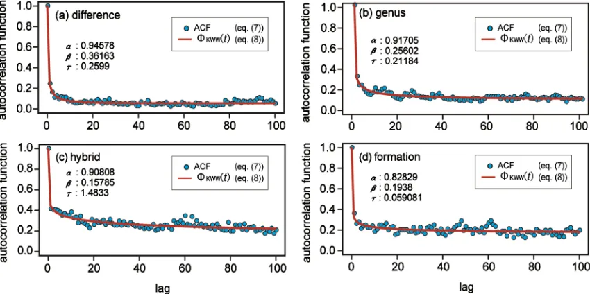
Figure 2, the ACFs in Figure 2 are well described by Equation (12), as indicated by all the curves in the figure. However, we found that there are many words showing dynamic correlations and having ACFs that are gradually decreasing but take positive finite values in the limit t→ ∞. Typical examples of such ACFs taken from the Darwin text are displayed in Figure 4. The positive finite values of ACFs as t→ ∞ cannot be represented by the original KWW function, Equation (12), because its limit value is zero. In order to extend the descriptive ability of the model function to ACFs with non-zero limit values, we introduced one additional parameter, α, to the original KWW function and defined the slightly modified ΦKWW

( )

t shown in Equation (8), which allows a limit value

of 1− >α 0 when t→ ∞. This modification ensures good fitting results for

[image:11.595.113.538.468.680.2]

ACFs showing dynamic correlations and having positive limit values, as seen in

Figure 4.

Another model function is ΦPoisson

( )

t , which is suitable for ACFs exhibiting

DOI: 10.4236/jdaip.2019.72004 57 Journal of Data Analysis and Information Processing no dynamic correlations, as in Figure 3. ΦPoisson

( )

t is defined as a stepdown

function:

( )

(

₍

)

₎

Poisson

1 0

0 t t

t γ

=  Φ _{= }

>

 (13)

where γ is a fitting parameter satisfying

0< <γ 1. ₍₁₄₎

For ACFs exhibiting no correlations, as in Figure 3, it is obvious that ΦPoisson

( )

t

is the one and the only expression needed.

In the fitting procedures using the two model functions, we found that the set of ΦKWW

( )

t and ΦPoisson

( )

t , Equations (8) and (13), offers full descriptive

ability for all the calculated ACFs: for example, when fitting using ΦPoisson

( )

t

gives a poor result, ΦKWW

( )

t provides a satisfactory fitting. We used the

pack-age “minpack.lm” in this study that provides an R interface to the non-linear least-squares fitting.

5.3. Classification of Frequent Words

Another important point to note is that these two expressions for ACFs, ΦKWW

( )

t

and ΦPoisson

( )

t , are not mutually exclusive. Rather, they are seamlessly

con-nected in the following sense. Substituting a very small value of τ such that

1

τ  into Equation (8) yields ΦKWW

( )

t ≅ − =1 α constant for t≥1.

Com-bining this fact with ΦKWW

( )

0 =1 leads us to an understanding of the nested

relationship between ΦKWW

( )

t and ΦPoisson

( )

t : ΦPoisson

( )

t is formally

in-cluded in the expression of ΦKWW

( )

t as the special case τ→0. This means

that if ΦPoisson

( )

t gives a satisfactory fitting, thenΦKWW

( )

t with a small value

of τ is also suitable to describe the ACF. An example of such a situation is shown in Figure 5, indicating that both ΦKWW

( )

t and ΦPoisson

( )

t give good

fitting results for the ACF of the word “subject” in the Darwin text. Based on the results shown in Figure 5, it might be thought that the model function ΦPoisson

( )

t

is not necessary because ΦKWW

( )

t gives satisfactory fittings not only for

dy-namically correlated ACFs, as in Figure 2, but also for non-correlated ones, as in

[image:12.595.117.540.582.689.2]

Figure 5(a). However, this is not true because of the following two principles of model selection. First, the theory of statistical model selection tells us that, given

Figure 5. Fitting results for the ACF of “subject” in the Darwin text. (a) The result using ΦKWW

( )

t (b) that using

( )

Poisson t

DOI: 10.4236/jdaip.2019.72004 58 Journal of Data Analysis and Information Processing candidate models of similar explanatory power, the simplest model is most likely to be the best choice [29]. In the case of Figure 5, we should thus choose

( )

Poisson t

Φ _{, which has one fitting parameter, as the better model rather than}

( )

KWW t

Φ _{, which has three parameters. Second, we should reject any model if} the values of the best fit parameters make no sense [29]. With regard to this point, the fitting in Figure 5(a) is obviously inappropriate because the value of the fitting parameter τ_{≅1.72 10×} −7, which is formally interpreted as a

“relaxa-tion time” of occurrence probability, is too small to represent real relaxa“relaxa-tion phe-nomena of word occurrences in the text. Consequently, the second principle also tells us that we should choose ΦPoisson

( )

t for describing the ACF of Figure 5.

Based on the two principles of model selection described above, we set three criteria for model selection through which the best model is determined from the two candidates, ΦKWW

( )

t and ΦPoisson

( )

t . If the ACF of a considered word

is best described by ΦKWW

( )

t in terms of the criteria, then the word is called a

“Type-I” word. If the best description is given by ΦPoisson

( )

t , then the word is

called a “Type-II” word. Type-I words are those words that have dynamic corre-lations, as in Figure 2 and Figure 4, while Type-II words have no dynamic cor-relations, as in Figure 3 and Figure 5.

The following criteria classify a word as Type-I or Type-II without any ambi-guity and are applied throughout the rest of this work.

(C1) After fitting procedures using both functions, ΦKWW

( )

t and ΦPoisson

( )

t ,

we evaluate the Bayesian information criterion (BIC) [30] [31] [32] for both cas-es. The BIC calculation formula used for our fitting results will be described in the next subsection. If the BIC of the fitting using ΦPoisson

( )

t , BIC(Poisson), is

smaller than the BIC of the fitting using ΦKWW

( )

t , BIC(KWW), then we judge

that ΦPoisson

( )

t is better for describing the ACF of a considered word and we

categorize the word as a Type-II word. This judgment using BIC is a more strict realization of the first principle described above.

(C2) If BIC(KWW) is smaller than BIC(Poisson) and the best fitted value of 𝜏𝜏 in ΦKWW

( )

t is smaller than 0.01, then we judge that ΦPoisson

( )

t is better and

we classify the considered word as a Type-II word. This judgment is a realization of the second principle, that is, we treat values of τ smaller than 0.01 as making no sense.

(C3) If BIC(KWW) is smaller than BIC(Poisson) and τ is greater than or equal to 0.01, then we judge that ΦKWW

( )

t is better and we classify the word as

a Type-I word.

DOI: 10.4236/jdaip.2019.72004 59 Journal of Data Analysis and Information Processing

( )

1 ,

e

τ

τ β

β = Γ

(15) where β and τ are the parameters in ΦKWW

( )

t and Γ denotes the gamma

func-tion. Substituting β =0.2 into the above equation, where 0.2 is a typical value

of β for Type-I words as can be seen in Figure 2 and Figure 4, and solving the in-equality τ_e >1.0 with Equation (15) for τ gives the condition τ>0.008333333.

From this result, we tentatively set the threshold value of τ as 0.01, and this value is used throughout this work.

We classified all frequent words into one of the two types according to the cri-teria (C1)-(C3). Table 3 summarizes the numbers of words belonging to each of the two types in our text set. The ratio of Type-I to Type-II words varied from text to text, but typically Type-I and Type-II words appeared in about the same pro-portion.

5.4. Model Selection Using the Bayesian Information Criterion As stated above, we used both of the two model functions, ΦKWW

( )

t and

( )

Poisson t

Φ _{, to describe each of the calculated ACFs and then determined which} model function to use by checking the criteria (C1)-(C3) for a considered ACF. In the determination, we used the Bayesian information criterion (BIC), which has been widely used as a criterion for model selection from among a finite set of models [30] [31] [32]. The BIC is formally defined for model M as

( )

ˆ

( )

( )

BIC M =nlnL M +kln n .

(16) where _Lˆ _{is the maximized value of the likelihood function of the model M, k is}

[image:14.595.198.540.494.737.2]

the number of fitting parameters to be estimated, and n is the number of data points. In a comparison of models, the model with the lowest BIC is chosen as

Table 3. Numbers of frequent words belonging to each of the two types.

Text Type-I (%) Type-II (%) Total

Carroll 5 (50.0) 5 (50.0) 10

Twain 11 (23.9) 35 (76.1) 46

Austen 13 (9.6) 123 (90.4) 136

Tolstoy 273 (34.3) 524 (65.7) 797

Melville 56 (23.6) 181 (76.4) 237

Darwin 109 (51.4) 103 (48.6) 212

Einstein 17 (70.8) 7 (29.2) 24

Lavoisier 99 (63.9) 56 (36.1) 155

Freud 14 (46.7) 16 (53.3) 30

Smith 384 (71.5) 153 (28.5) 537

Kant 143 (49.5) 146 (50.5) 289

DOI: 10.4236/jdaip.2019.72004 60 Journal of Data Analysis and Information Processing the best one. Under the assumption that model errors are independent and iden-tically distributed according to a normal distribution, the BIC can be rewritten as

( )

(

( )

)

2

( )

1

1 _ˆ

ˆ

BIC ln ln .

n

i i i

M n x x M k n

n = θ

 

=  − +



∑

 (17)

where xi is the i-th data point, xˆi the predicted value of xi by model M, and

( )

ˆ _M

θ _{is the vector of parameter values of model M optimized by the} curve-fitting procedures. In the above equation, we have omitted an additive constant that depends on only n and not on the model M.

For our application, M is KWW or Poisson, xi the ACF of a considered word calculated with Equation (7) at the i-th lag step, xˆ_i is the predicted value of the ACF given by ΦKWW

( )

t or ΦPoisson

( )

t at t=i, the parameter vector is

(

) (

)

ˆ KWW , ,

θ = α β τ _or θˆ Poisson

(

)

=γ _{, the numbers of parameters are}

(

KWW

)

3

k = or k

(

Poisson

)

=1, and n = 100, which represents the maximum

lag step used in the ACF calculation. We evaluated BIC(KWW) and BIC(Poisson) by use of Equation (17) and classified a considered word as Type-I or Type-II ac-cording to the criteria (C1)-(C3) described above. That is, if BIC(KWW) < BIC(Poisson) and τ≥0.01, then we judge that ΦKWW

( )

t is the better model

and we classify the word as a Type-I word, otherwise ΦPoisson

( )

t is the better

model and we classify the word as Type-II. 5.5. Stochastic Model for Type-II Words

We consider here a stochastic model for Type-II words and attempt to derive

( )

Poisson t

Φ _{, which is the model equation used for ACFs of Type-II words. We} first assume that the observation count Xt of a considered Type-II word in the first t sentences of a text obeys a homogeneous Poisson point process. This is because the process is the simplest one having the property that disjoint time in-tervals are completely independent of each other, and this property makes the process suitable for the Type-II case which does not show any dynamical corre-lations. Then, the probability of k observations of the word in t sentences is giv-en by

(

) ( )

exp

( )

. !

k

t

t

P X k t

k λ

λ

= = −

(18) where λ is the rate of word occurrences (occurrence probability per sentence) and the mean of Xt is given by E X

[ ]

t =λt [14]. Since the binary variable of word occurrence, A t

( )

defined by Equation (4), can be expressed in terms of

t X as

( )

t t 1,

A t =X −X− ₍₁₉₎ the mean of A t

( )

turns out to be

( )

[ ] [

t t 1

]

(

1

)

. E A t_ _=E X −E X₋ =λ λt− t− =λ

(20)

DOI: 10.4236/jdaip.2019.72004 61 Journal of Data Analysis and Information Processing

( )

( ) (

)

( )

(

)

2 .

E A t A t s s

E A t

+     Φ =       (21)

The above definition is essentially the same as Equation (2) for ergodic sys-tems in which expectation values can be replaced by time averages [24]. We will derive the ACF for the homogeneous Poisson point process from Equation (21). Noting that the numbers of occurrences in disjoint intervals are independent random variables for the homogeneous Poisson point process, the numerator of Equation (21) becomes

( ) (

)

( )

(

)

2

. E A t A t_ +s _=E A t_  _{ }E A t+s _=λ

(22) where we have used Equation (20) and the stationary property,

( )

(

)

E A t_ _=E A t_ +s _. For the denominator of Equation (21), we obtain

( )

(

)

2

(

( )

)

₂

(

( )

)

₂

(

( )

)

1 1 0 0 1 .

E_ A t  =_ P A t = × +P A t = × =P A t = =λ

(23) The first equality holds because A t

( )

is either 0 or 1, and the last equality holds because we assume that the occurrence rate (occurrence probability per unit time) is λ. Substituting Equations (22) and (23) into Equation (21) yields an expression for Φ

( )

s ,

( )

1

(

₍

0

)

₎

0 s s s λ =  Φ _{= }

>

 (24)

which is equivalent to ΦPoisson

( )

t given by Equation (13). Since λ is the rate

constant of the homogeneous Poisson point process, it can be simply evaluated from real written text by

number of sentences containing a considered word

ˆ _,

number of all sentendes in text

λ=

(25) and the evaluated _λˆ _{can be directly compared with the fitting parameter γ in} Equation (13) to confirm the validity of the discussion above.

Figure 6 shows a scatter plot of _λˆ _{evaluated by Equation (25) versus the} best-fit parameter γ of ΦPoisson

( )

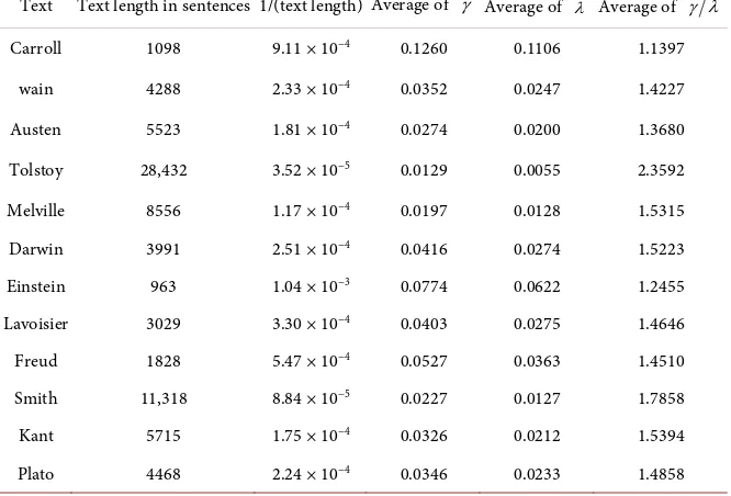
t for all Type-II words in the considered texts.

DOI: 10.4236/jdaip.2019.72004 62 Journal of Data Analysis and Information Processing The influence of the short window size of lag steps mentioned above is evident in Figure 7, which displays the relationship between the average value of _{γ λ}ˆ

for Type-II words in each text and the inverse of the text length. The values used in Figure 7 are tabulated in Table 4. It follows from Figure 7 that the average value of _{γ λ}ˆ _{gradually approaches the limit value of 1 as the text length}

be-comes shorter. This indicates that the influence of the short window size in eva-luating γ reasonably becomes smaller as the ratio of the window size to the text length becomes larger. The overall behavior of γ vs. _λˆ_{, plotted in Figure 6, and} the additional information supplied by Figure 7 convince us that the derivation

of ΦPoisson

( )

t based on the properties of the homogeneous Poisson point

process described above is fundamentally correct.

[image:17.595.267.481.335.488.2]

Through the discussion on Type-II words described above, we can recognize that the value of the fitting parameter γ in Equation (13) carries important in-formation: γ is the estimator for the rate constant of the homogeneous Poisson point process. This is the reason for employing Equation (2) as the starting point of the normalized ACF. If we employ Equation (3) instead of Equation (2), then all the ACFs of Type-II words become Φ

( )

0 =1 and Φ >

(

t 0

)

=0, without

Figure 6. Comparison of _λˆ _{evaluated by Equation (25) and the best-fit parameter γ in} Equation (13) for Type-II words in the Darwin, Twain, Freud, Lavoisier and Austen texts. The dashed line represents the relation _{γ λ=} ˆ_.

[image:17.595.238.509.544.692.2]

[image:18.595.207.540.101.327.2]

DOI: 10.4236/jdaip.2019.72004 63 Journal of Data Analysis and Information Processing Table 4. Average values of γ _{, λ}ˆ _{and γ λ}ˆ _{for Type-II words from each text.}

Text Text length in sentences 1/(text length) Average of γ _{Average of λ}ˆ _{Average of γ λ}ˆ

Carroll 1098 9.11 × 10−4 _{0.1260 0.1106 1.1397}

wain 4288 2.33 × 10−4 _{0.0352 0.0247 1.4227}

Austen 5523 1.81 × 10−4 _{0.0274 0.0200 1.3680}

Tolstoy 28,432 3.52 × 10−5 _{0.0129 0.0055 2.3592}

Melville 8556 1.17 × 10−4 _{0.0197 0.0128 1.5315}

Darwin 3991 2.51 × 10−4 _{0.0416 0.0274 1.5223}

Einstein 963 1.04 × 10−3 _{0.0774 0.0622 1.2455}

Lavoisier 3029 3.30 × 10−4 _{0.0403 0.0275 1.4646}

Freud 1828 5.47 × 10−4 _{0.0527 0.0363 1.4510}

Smith 11,318 8.84 × 10−5 _{0.0227 0.0127 1.7858}

Kant 5715 1.75 × 10−4 _{0.0326 0.0212 1.5394}

Plato 4468 2.24 × 10−4 _{0.0346 0.0233 1.4858}

exception, and thus they become useless for getting information about the un-derlying homogeneous Poisson point process.

5.6. Measure of Dynamic Correlation

We have seen that frequent words can be classified as Type-I or Type-II words. Obviously, Type-I words, having dynamic correlations, are more important for a text because each of them appears multiple times in a bursty manner to describe a certain idea or a topic, which can be important for the text. In contrast, each of the Type-II words without dynamic correlations appears at an approximately constant rate in accordance with the homogeneous Poisson point process and therefore they cannot be related to any context in the text. The natural question arising from the discussion above is how we measure the importance of each word in terms of dynamic correlations.

As described earlier, we judged whether a word is Type-I or Type-II by using criteria (C1), (C2), and (C3) in which comparing BIC (KWW) and BIC (Poisson) plays a central role for the judgment. We introduce here a new quantity, ΔBIC, for Type-I words with the hope of quantifying the importance of each word. ΔBIC is defined as the difference between BIC KWW) and BIC (Poisson) for each Type-I word;

(

)

(

)

BIC BIC Poisson BIC KWW .

∆ = −

(26) This value expresses the extent to which the best fitted ΦKWW

( )

t is different

from the best fitted ΦPoisson

( )

t in terms of their overall functional behaviors.

Since we have already seen that ΦPoisson

( )

t is the ACF of the homogeneous

[image:19.595.204.537.369.730.2]

DOI: 10.4236/jdaip.2019.72004 64 Journal of Data Analysis and Information Processing an intuitive measure expressing the degree of dynamic correlation for Type-I words. In other words, ΔBIC describes the extent to which the stochastic process that governs the occurrences of the considered word deviates from a homoge-neous Poisson point process. Note that ΔBIC always takes positive values be-cause we define it only for Type-I words. Thus, a larger ΔBIC indicates that a word has a stronger dynamical correlation. The authors have already developed a measure of deviation from a Poisson distribution for static word-frequency distributions in written texts and have used that measure for text-classification tasks [35] [36] [37]. Although ΔBIC is very different from the definition of the static measure that was developed, the basic idea behind them is similar because ΔBIC can be regarded as a dynamical version of a measure of deviation from a Poisson distribution.

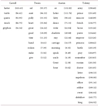
Table 5 summarizes the top 20 Type-I words in terms of ΔBIC for our text set. Each of these words seems to be plausible in the sense that it is a keyword that plays a central role in describing a certain idea or topic, and so it should appear multiple times when the author explains the idea or the topic in the text, and this appearance should be over, typically, several to several tens of sentences. The plausibility is more pronounced in academic books (Darwin, Einstein, Lavoisier,

Table 5. Top 20 Type-I words in terms of ΔBIC. The values of ΔBIC are shown in parentheses.

Carroll Twain Austen Tolstoy

DOI: 10.4236/jdaip.2019.72004 65 Journal of Data Analysis and Information Processing

Melville Darwin Einstein Lavoisier

whale (238.84) intermediate (237.47) theory (107.63) acid (265.54) boat (176.84) variety (197.75) gravitational (89.66) ord (248.30) captain (167.21) specie (189.99) velocity (85.01) caloric (245.81) thou (149.44) plant (185.22) field (82.42) metal (217.58) ahab (148.56) seed (184.80) motion (79.29) mercury (205.74) pip (142.50) area (179.06) point (73.41) gas (193.47) spout (139.54) organ (174.80) coordinate (72.91) water (187.70) line (124.37) bird (174.07) principle (71.27) combustion (183.23) jonah (113.52) flower (167.41) body (67.05) body (176.02) masthead (112.86) form (162.20) law (61.30) sulphur (168.42) sperm (111.84) instinct (160.27) time (59.83) tube (165.41) bildad (110.36) character (158.87) relativity (56.62) air (164.38) flask (110.09) nest (158.22) system (54.48) temperature (152.40) oil (108.19) rudimentary (154.39) light (45.90) muriatic (147.60) tail (101.13) bee (147.35) general (33.84) ice (144.32) queequeg (98.87) variability (146.35) relative (27.94) pound (141.17) harpooner (96.33) tree (142.90) space (14.51) oxygen (138.28) fish (93.78) island (142.13) distillation (126.75) carpenter (90.69) rank (136.06) charcoal (125.45) dick (90.48) selection (132.83) nitric (124.40)

Freud Smith Kant Plato

dream (243.18) price (350.17) judgement (299.96) opinion (138.90) thought (130.91) labour (296.21) conception (259.94) knowledge (127.24) sleep (128.58) profit (286.68) reason (253.09) evil (119.59) sexual (112.75) trade (270.55) object (241.06) state (112.76) unconscious (83.93) country (269.82) experience (229.76) justice (107.34) system (76.47) revenue (265.82) time (225.28) class (95.16)

DOI: 10.4236/jdaip.2019.72004 66 Journal of Data Analysis and Information Processing Freud, Smith, Kant, and Plato) than in novels (Carroll, Twain, Austen, Tolstoy, and Melville). This is probably because the word to characterize a certain topic is more context-specific in academic books than in novels.

To confirm the validity of using ΔBIC to measure the deviation from a ho-mogeneous Poisson point process, we have attempted to apply another measure of the deviation to our text set, and have examined whether the relation between ΔBIC and this other measure can be interpreted in a uniform and consistent manner. We chose Kleinberg’s burst detection algorithm [38] for this purpose because this algorithm can clearly describe the extent to which a process go-verning the occurrences of a considered word deviates from a homogeneous Poisson point process, and so the results of the algorithm can be easily compared to ΔBIC, as will be described below. Furthermore, since the mathematical foun-dation of Kleinburg’s algorithm is completely different from ours, the validity of using ΔBIC will be strongly supported if the results of the algorithm are closely and consistently related to those of ΔBIC.

The Kleinburg’s algorithm analyzes the rate of increase of word frequencies and identifies rapidly growing words by using a probabilistic automaton. That is, it assumes an infinite number of hidden states (various degrees of burstiness), each of which corresponds to a homogeneous Poisson point process having its own rate parameter, and the change of occurrence rate in a unit time interval is modeled as a transition between these hidden states. The trajectory of state tran-sition is determined by minimizing a cost function, where it is expensive (costly) to go up a level and cheap (zero-cost) to go down a level.

[image:22.595.184.540.68.358.2]

DOI: 10.4236/jdaip.2019.72004 67 Journal of Data Analysis and Information Processing Figure 8. Results of Kleinburg’s burst detection algorithm. The left and right columns show results for the word “organ” and those for the word “reason”, respectively, which are taken from Darwin text. (a) and (d): Cumulative counts of word occurrences through text; (b) and (e): Burst-level variations predicted by the Kleinburg’s algorithm; (c) and (f): ACFs for “organ” and “reason”. Making their non-Poisson and Poisson natures apparent.

were detected by Kleinburg’s algorithm. For Figure 8(b) and Figure 8(e), these cumulative counts of transitions are 30 and 0, respectively. Note that if the level changes from 1 to 2 and then goes down from 2 to 1, the number of level transi-tions is two.

Figure 9 shows scatter plots of the cumulative counts of transitions (abbre-viated as CCT) in the results of Kleinberg’s algorithm versus ΔBIC for our entire text set, where we used all Type-I words in each text. The scatter plots show an obvious positive correlation between ΔBIC and CCT for all texts, though the de-gree of correlation depends on the text. For further quantitative analysis, we calculated correlation coefficients between ΔBIC and CCT and performed a sta-tistical test of the null hypothesis “the true correlation coefficient is equal to ze-ro”. Table 6 summarizes the results, showing that, except for the text of Carroll, all the texts have a statistically significant positive correlation between ΔBIC and CCT, with correlation coefficients ranging from about 0.7 to about 0.9. The null hypothesis cannot be rejected for the Carroll text when we set the significance level to α =5%. Obviously, the sample size, n=5, is too small to obtain

[image:23.595.54.544.131.719.2]

DOI: 10.4236/jdaip.2019.72004 68 Journal of Data Analysis and Information Processing ΔBIC serves as a measure of deviation from a Poisson point process. In addition, ΔBIC can be a more precise measure than CCT in the sense that it takes conti-nuous real values while the CCT takes only discrete integer values. For example, 9 words have CCT = 4 in the Einstein text, and we can easily assign ranks to

[image:24.595.208.539.101.321.2]

DOI: 10.4236/jdaip.2019.72004 69 Journal of Data Analysis and Information Processing Table 6. Correlation coefficients between ΔBIC and CCT and the results of “no correla-tion” tests. The data used in the computations are the same as those used in Figure 9.

Text Correlation coefficient p-value

Carroll 0.619 2.65 × 10−1

Twain 0.966 1.46 × 10−6

Austen 0.804 9.14 × 10−4

Tolstoy 0.746 2.20 × 10−16

Melville 0.810 4.09 × 10−13

Darwin 0.864 2.20 × 10−16

Einstein 0.727 9.49 × 10−4

Lavoisier 0.874 2.20 × 10−16

Freud 0.625 1.69 × 10−2

Smith 0.781 2.20 × 10−16

Kant 0.831 2.20 × 10−16

Plato 0.735 6.85 × 10−8

these 9 words by use of ΔBIC, as seen in the scatter plot for the Einstein text in

Figure 9(g).

Furthermore, we consider that ΔBIC can be used to measure the importance of a considered word in a given text because it expresses the extent to which the word occurrences are correlated with each other among successive sentences, and a large ΔBIC means that the word occurs multiple times in a bursty and context-specific manner. Of course, there can be various viewpoints to judge word importance; but at least ΔBIC offers well-defined procedures for calcula-tion, with a clear meaning in terms of the stochastic properties of word occur-rence. In this sense, ΔBIC has a wide range of real applications in which the de-gree of importance of each word is required.

6. Conclusions

DOI: 10.4236/jdaip.2019.72004 70 Journal of Data Analysis and Information Processing words, and their ACFs are modeled by a simple stepdown function. For the model function of Type-II words, we have shown that the functional form of the simple stepdown function can be theoretically derived from the assumption that the stochastic process governing word occurrence is a homogeneous Poisson point process. To select the appropriate type for a word, we have used the Baye-sian information criterion (BIC).

We further proposed a measure of word importance, ΔBIC, which was de-fined as the difference between the BIC using the KWW function and that using the stepdown function. If ΔBIC takes a large value, then the stochastic process governing word occurrence is considered to deviate greatly from the homoge-neous Poisson point process (which does not produce any correlations between two arbitrary separated time intervals). This indicates that a word with large ΔBIC has strong dynamic correlations with some range of duration along the text and is, therefore, important for a considered text. We have picked the top 20 Type-I words in terms of ΔBIC for each of the 12 texts, and found that the re-sultant word list seems to be plausible, especially for academic books. The valid-ity of using ΔBIC to measure word importance was confirmed by comparing the value of ΔBIC with another measure of word importance. We chose the CCT as the other measure. This was obtained by applying the Kleinburg’s burst detec-tion algorithm. We found that CCT and ΔBIC show a strong positive correladetec-tion. Since the backgrounds of CCT and that of ΔBIC are completely different from each other, the strong positive correlation between them means that both the CCT and ΔBIC are useful ways to measure the importance of a word.

At present, the stochastic process that governs dynamic correlations of Type-I words with long-range duration time is not clear. A detailed study along this line, through which we will try to identify the process suitable to describe word oc-currences in real texts, is reserved for future work.

Acknowledgements

We thank Dr. Yusuke Higuchi for useful discussion and illuminating suggestions. This work was supported in part by JSPS Grant-in-Aid (Grant No. 25589003 and 16K00160).

Conflicts of Interest

The authors declare no conflicts of interest regarding the publication of this pa-per.

References

[1] Bullinaria, J.A. and Levy, J.P. (2007) Extracting Semantic Representations from Word Co-Occurrence Statistics: A Computational Study. Behavior Research

Me-thods, 39, 510-526.https://doi.org/10.3758/BF03193020

[2] Matsuo, Y. and Ishizuka, M. (2004) Keyword Extraction from a Single Document Using Word Co-Occurrence Statistical Information. International Journal on

DOI: 10.4236/jdaip.2019.72004 71 Journal of Data Analysis and Information Processing

[3] Rose, N.C.S., Engel, D. and Cowley, W. (2010) Automatic Keyword Extraction from Individual Documents. In: Berry, M.W. and Kogan, J., Eds., Text Mining:

Applica-tions and Theory, Chapter 1, John Wiley & Sons, Hoboken, 3-20.

https://doi.org/10.1002/9780470689646

[4] Bordag, S. (2008) A Comparison of Co-Occurrence and Similarity Measures as Si-mulations of Context. Springer, Berlin, Heidelberg, 52-63.

https://doi.org/10.1007/978-3-540-78135-6_5

[5] Terra, E. and Clarke, C.L.A. (2003) Frequency Estimates for Statistical Word Simi-larity Measures. Proceedings of the Conference of the North American Chapter of

the Association for Computational Linguistics on Human Language Technology,

Vol. 1, Edmonton, 27 May-1 June 2003, 165-172.

https://doi.org/10.3115/1073445.1073477

[6] Zhang, J., Schenkel, A. and Zhang, Y.-C. (1993) Long Range Correlation in Human Writings. Fractals, 1, 47-57.https://doi.org/10.1142/S0218348X93000083

[7] Ebeling, W. and Poschel, T. (1994) Entropy and Long-Range Correlations in Lite-rary English. Euro-Physics Letters, 26, 241.

https://doi.org/10.1209/0295-5075/26/4/001

[8] Perakh, M. (2012) Serial Correlation Statistics of Written Texts. International

Jour-nal of ComputatioJour-nal Linguistics and Applications, 3, 11-43.

[9] Motter, A.E., Altmann, E.G. and Pierrehumbert, J.B. (2009) Beyond Word Fre-quency: Bursts, Lulls, and Scaling in the Temporal Distributions of Words. PLoS ONE, 4, e7678.https://doi.org/10.1371/journal.pone.0007678

[10] Montemurro, M.A. and Pury, P.A. (2002) Long-Range Fractal Correlations in Lite-rary Corpora. Fractals, 10, 451-461.https://doi.org/10.1142/S0218348X02001257

[11] Sarkar, A., Garthwaite, P.H. and De Roeck, A. (2005) A Bayesian Mixture Model for Term Re-Occurrence and Burstiness. Ninth Conference on Computational

Lan-guage Learning, Ann Arbor, 29-30 June 2005, 48-55.

https://doi.org/10.3115/1706543.1706552

[12] Alvarez-Lacalle, E., Dorow, B., Eckmann, J.-P. and Moses, E. (2006) Hierarchical Structures Induce Long-Range Dynamical Correlations in Written Texts.

Proceed-ings of the National Academy of Sciences of the United States of America, 103,

7956-7961.https://doi.org/10.1073/pnas.0510673103

[13] Cristadoro, G., Altmann, E.G. and Esposti, M.D. (2012) On the Origin of Long-Range Correlations in Texts. Proceedings of the National Academy of Sciences of the

United States of America, 109, 1582-11585.

https://doi.org/10.1073/pnas.1117723109

[14] Taylor, H.M. and Karlin, S. (1994) An Introduction to Stochastic Modeling. Aca-demic Press, Cambridge.https://doi.org/10.1016/B978-0-12-684885-4.50007-0

[15] Khvatskin, L.V., Frenkel, I.B. and Gertsbakh, I.B. (2003) Parameter Estimation and Hypotheses Testing for Nonhomogeneous Poisson Process. Transport and

Tele-communication, 4, 9-17.

[16] National Institute of Standards and Technology (2013) e-Handbook of Statistical Methods. http://www.itl.nist.gov/div898/handbook

[17] Tang, M.-L., Yua, J.-W. and Tianb, G.-L. (2007) Predictive Analyses for Nonhomo-geneous Poisson Processes with Power Law Using Bayesian Approach.

Computa-tional Statistics & Data Analysis, 51, 4254-4268.

https://doi.org/10.1016/j.csda.2006.05.010

DOI: 10.4236/jdaip.2019.72004 72 Journal of Data Analysis and Information Processing

Text. Literary and Linguistic Computing, 8, 20-26.https://doi.org/10.1093/llc/8.1.20

[19] Roberts, A. (1996) Rhythm in Prose and the Serial Correlation of Sentence Lengths: A Joyce Cary Case Study. Literary & Linguistic Computing, 11, 33-39.

https://doi.org/10.1093/llc/11.1.33

[20] Pawlowski, A. (1997) Time-Series Analysis in Linguistics. Application of the Arima Method to Some Cases of Spoken Polish. Journal of Quantitative Linguistics, 4, 203-221.https://doi.org/10.1080/09296179708590097

[21] Pawlowski, A. (1999) Language in the Line vs. Language in the Mass: On the Effi-ciency of Sequential Modelling in the Analysis of Rhythm. Journal of Quantitative

Linguistics, 6, 70-77.https://doi.org/10.1076/jqul.6.1.70.4140

[22] Pawlowski, A. (2005) Modelling of Sequential Structures in Text. In: Handbooks of

Linguistics and Communication Science, Walter de Gruyter, Berlin, 738-750.

[23] Pawlowski, A. and Eder, M. (2015) Sequential Structures in “Dalimil’s Chronicle”. In: Mikros, G.K. and Macutek, J., Eds., Sequences in Language and Text, Volume 69 of Quantitative Linguistics, Walter de Gruyter, Berlin, 104-124.

[24] Dunn, P.F. (2010) Measurement, Data Analysis, and Sensor Fundamentals for En-gineering and Science. 2nd Edition, CRC Press, ‎Boca Raton.

https://doi.org/10.1201/b14890

[25] Kulahci, M., Montgomery, D.C. and Jennings, C.L. (2015) Introduction to Time Se-ries Analysis and Forecasting. 2nd Edition, John Wiley & Sons, Hoboken.

[26] Salton, G. (1971) The SMART Retrieval System—Experiments in Automatic Doc-ument Processing. Prentice-Hall Inc., Upper Saddle River.

[27] R-Core-Team (2014) R: A Language and Environment for Statistical Computing. R Foundation for Statistical Computing, Vienna. http://www.R-project.org

[28] Elton, D.C. (2018) Stretched Exponential Relaxation.

[29] Motulsky, H. and Christopoulos, A. (2004) Fitting Models to Biological Data Using Linear and Non-Linear Regression; a Practical Guide to Curve Fitting. Oxford Uni-versity Press, Oxford.

[30] Konishi, S. and Kitagawa, G. (2007) Information Criteria and Statistical Modeling. Springer, Berlin.https://doi.org/10.1007/978-0-387-71887-3

[31] Burnham, K.P. and Anderson, D.R. (2004) Multimodel Inference; Understanding AIC and BIC in Model Selection. Sociological Methods and Research, 33, 261-304.

https://doi.org/10.1177/0049124104268644

[32] Ogura, H., Amano, H. and Kondo, M. (2014) Classifying Documents with Poisson Mixtures. Transactions on Machine Learning and Artificial Intelligence, 2, 48-76.

https://doi.org/10.14738/tmlai.24.388

[33] Bailey, N.P. (2009) A Memory Function Analysis of Non-Exponential Relaxation in Viscous Liquids.

[34] Zatryb, G., Podhorodecki, A., Misiewicz, J., Cardin, J. and Gourbilleau, F. (2011) On the Nature of the Stretched Exponential Photoluminescence Decay for Silicon Na-nocrystals. Nanoscale Research Letters, 6, 1-8.

https://doi.org/10.1186/1556-276X-6-106

[35] Ogura, H., Amano, H. and Kondo, M. (2009) Feature Selection with a Measure of Deviations from Poisson in Text Categorization. Expert Systems with Applications, 36, 6826-6832.https://doi.org/10.1016/j.eswa.2008.08.006

[36] Ogura, H., Amano, H. and Kondo, M. (2010) Distinctive Characteristics of a Metric Using Deviations from Poisson for Feature Selection. Expert Systems with

DOI: 10.4236/jdaip.2019.72004 73 Journal of Data Analysis and Information Processing

[37] Ogura, H., Amano, H. and Kondo, M. (2011) Comparison of Metrics for Feature Selection in Imbalanced Text Classification. Expert Systems with Applications, 38, 4978-4989.https://doi.org/10.1016/j.eswa.2010.09.153

[38] Kleinberg, J. (2002) Bursty and Hierarchical Structure in Streams. Proceedings of

the 8th ACM SIGKDD International Conference on Knowledge Discovery and Data