On the late-time behaviour of a bounded,
inviscid two-dimensional flow
David G. Dritschel
1†
, Wanming Qi
2,3,4and J. B. Marston
3,41
School of Mathematics and Statistics, University of St Andrews, St Andrews KY16 9SS, UK
2
School of Physics, Korea Institute for Advanced Study, Seoul 130-722, Korea
3
Kavli Institute for Theoretical Physics, University of California, Santa Barbara, CA 93106-4030 USA
4
Department of Physics, Brown University, Providence, RI 02912-1843, USA
(Received ?; revised ?; accepted ?. - To be entered by editorial office)
Using complementary numerical approaches at high resolution, we study the late-time behaviour of an inviscid, incompressible two-dimensional flow on the surface of a sphere. Starting from a random initial vorticity field comprised of a small set of intermediate wavenumber spherical harmonics, we find that — contrary to the predictions of equi-librium statistical mechanics — the flow does not evolve into a large-scale steady state. Instead, significant unsteadiness persists, characterised by a population of persistent small-scale vortices interacting with a large-scale oscillating quadrupolar vorticity field. Moreover, the vorticity develops a stepped, staircase distribution, consisting of nearly homogeneous regions separated by sharp gradients. The persistence of unsteadiness is explained by a simple point vortex model characterising the interactions between the four main vortices which emerge.
1. Introduction
Two-dimensional flow models have often been used as an idealised description of atmo-spheric and oceanic fluid dynamics. These models afford the maximum simplicity while retaining the key advective nonlinearity of fluid motion and the associated scale cascade. However, such models fail to capture the intrinsic three-dimensionality of atmospheric and oceanic flows at ‘small’ scales, where the effects of rotation and stratification strongly compete (Dritschelet al.1999). Nevertheless, mathematically, much interest remains in understanding how nonlinearity organises fluid motion in this simple context.
In this paper, we examine the behaviour of a bounded two-dimensional incompressible inviscid (dissipationless) flow at long timest. The flow evolves freely from some prescribed initial condition, which is subsequently transformed by nonlinearity. No forcing is applied. This problem has been the subject of much previous research. Almost all laboratory experiments and numerical simulations have indicated a final state consisting of a steady large-scale circulation pattern filling the whole domain (see Matthaeus et al.(1991b,a); Montgomeryet al. (1992, 1993); Brands et al. (1997); Bouchet & Venaille (2012) for a sample of the vast literature). Unsteady final states have also been reported in several nu-merical simulations for doubly-periodic planar domains. Here, often two opposite-signed vortices emerge (see Qi & Marston (2014) & refs.). Segre and Kida found various unsteady final states using initial configurations of constant-vorticity patches (Segre & Kida 1998), but the simulations appear not to have gone far enough in time for the proper final state
Robert (1991), hereafter ‘MRS’. (Reviews may be found in Chavanis (2002); Eyink & Sreenivasan (2006); Majda & Wang (2006); Chavanis (2009); Bouchet & Venaille (2012); Herbert (2013); Qi & Marston (2014).) The MRS theory predicts that the nonlinear dynamics, characterised by intense turbulent mixing, ultimately results in a stationary large-scale, domain-filling flow. Moreover, this flow is obtained as a statistical mechani-cal equilibrium (assuming random fluctuations of fine-smechani-cale vorticity) dependent only on the inviscid invariants. Those include energy, circulation, and in general an infinite set of ‘Casimirs’ that determine the occupation of vorticity ω of each level within the fluid (this is the ‘vorticity measure’).
Verification of the MRS theory has met with mixed success (Qi & Marston 2014). The theory itself is difficult to work with when many Casimirs are taken into account, and vari-ous simplifications have been put forth (see e.g. the review by Bouchet & Venaille (2012)). Verification is also problematic when nearly all of the numerical methods used suffer from some form of dissipation, artificial or real, not present in the original inviscid system for which the theory was developed. A few numerical methods have been developed that conserve many invariants, including the Casimirs (Abramov & Majda 2003; Dubinkina & Frank 2010). Note that as numerical simulations inevitably have finite resolution, the Casimirs or the vorticity field observed numerically are only thecoarse-grained correspon-dence of those quantities of the inviscid system: the resolved vorticity field corresponds to the coarse-grained vorticity ¯ω, notω, and the second- and higher-order Casimirs of the resolved vorticity are different from the original fine-grained ones dependent onω. These conservative numerical methods would appear to be ideal, and moreover they would overcome the long-standing problem of how unresolved scales impact resolved ones, the ‘closure problem’. However, an irrefutable feature of two-dimensional turbulence is the enstrophy cascade, occurring as thin vorticity filaments stretch and thin to ever finer scales. By conservation, this cascade is necessary to build up energy at ever larger scales through an ‘inverse cascade’ (Fjørtoft 1953; Dritschel et al.2009, & refs.), as indeed is anticipated in the MRS theory. That is, energy growth at large scales requires a cascade of enstrophy to small scales. Since the Casimirs involve integrals of powers of the vortic-ity distribution, all but the first power (the circulation) cannot be even approximately conserved at any finite resolution, after sufficiently long time. Forcing conservation of quantities which cannot be conserved can only lead to spurious conclusions.
Verification of the MRS theory is further problematic because the invariantfine-grained
Casimirs that the theory depends on cannot be measured from any numerical simulation of finite resolution. However in practice the resolved Casimirs are often used to determine the values of the fine-grained Casimirs (at most approximately). Notably, the coarse-grained vorticity field ¯ωpredicted by the MRS theory often agrees with that emerging at large times in numerical simulations, if the late-time values of the resolved Casimirs are applied. Still these resolved Casimirs are not conserved and cannot be predicted from an arbitrary initial flow state of a numerical simulation, which limits the predictive power of the MRS theory.
equi-probable states with the same conserved quantities equate to time averages of a single state over a sufficiently long period of time. Two-dimensional flows are generally not ergodic (Whitaker & Turkington 1994; Bricmont et al. 2001; Bouchet & Corvellec 2010), though they are assumed to be in the MRS theory. It has been argued that MRS theory may still apply to states which exhibit strong turbulent mixing over the course of their evolution, e.g. to initially small-scale isotropic vorticity fields. There are many such states. But it is unclear whether they satisfy ergodicity even approximately.
The present paper is not intended to be a critique only of MRS theory; rather, we wish to present fresh evidence that even the central claim for the existence of a final steady equilibrium vorticity distribution ¯ω is likely to be false. Instead of the much studied doubly periodic planar domain, we consider flows on the sphere where statistical mechanics has not seen much application. While we agree that one can never carry out numerical simulations to infinite time, our results strongly suggest that, at least for flows on a sphere, unsteadiness persists for all time. Note that both Segre & Kida (1998) and Morita (2011) have focused on the type of final unsteadiness that is a result of special initial conditions (or insufficiently developed turbulence), but we argue that unsteadiness is generic by using a random initial state that generates fairly strong turbulent mixing: the unsteadiness is intrinsic to a system of compact coherent vortices. Our simulations are carried out much further in time and at much higher resolutions compared to the two studies, and the robustness of our result is verified by comparing two very different numerical approaches with fundamentally different forms of numerical dissipation.
The paper is organised as follows. In the next section, we briefly review the equa-tions and the associated conserved quantities, then describe two very different numerical methods employed. Both methods are used in §3 at many different resolutions, on the same initial data, to study the long-time convergence of the results. A few conclusions are offered in§4.
2. Governing equations and numerical methods
2.1. Two-dimensional flow on a sphereWe wish to study a freely-evolving incompressible two-dimensional flow, with no forcing or dissipation, confined to the surface of a unit sphere centered at the origin. In this case, the scalar vorticityω normal to the surface is materially conserved,
Dω Dt =
∂ω
∂t +u· ∇ω= 0, (2.1)
where u =r×∇ψ is the incompressible velocity field, r is the position of a point on
the surface (|r|= 1), andψis the scalar streamfunction. With∇ ·u= 0, the definition
ω=r·(∇×u) yields Poisson’s equation forψ:
∇2
ψ=ω . (2.2)
These equations were originally derived by Zermelo (1902) and Charney (1949). 2.2. Constants of the motion
Inviscid two-dimensional flow is an infinite-order Hamiltonian system with the kinetic energy
E= 1 2
Z Z
|u|2dΩ =−12
Z Z
ωψdΩ (2.3)
Cn=
Z Z
ωndΩ, n= 2,3, 4, ... (2.5)
are conserved. (C1= 0 automatically; no net circulation is possible on a closed surface).
TheCnare called the ‘Casimirs’. Their conservation is a consequence of the fact that the fractional area occupied by each vorticity value is conserved. For a continuous vorticity distribution, this fractional area is generally infinitesimal, and it is then useful to describe it as a ‘measure’, or probability densityp(ω): the area occupied by vorticity in the range [ω, ω+ dω] is 4πp(ω)dω. The conservation of all Cn is equivalent to the conservation of
p(ω).
The quadratic CasimirC2is proportional to the ‘enstrophy’Z(i.e.Z =C2/2). It plays a
key role in the so-called ‘dual cascade’ of two-dimensional turbulence, where nonlinearity generally results in a direct cascade of the spectral enstrophy density, enabling an inverse cascade of the spectral energy density (Fjørtoft 1953). This inverse cascade is often associated with the emergence of large-scale flow features, a general prediction of the MRS theory discussed in§1.
Beyond the conservation of an infinite number of Casimirs, Eq. (2.1) further implies the existence of a topological constraint that contours of vorticity cannot cross. This nonlocal constraint is usually ignored in the construction of statistical descriptions.
2.3. Numerical methods
Two very different numerical methods are used to cross verify our conclusions. The first is a purely grid-based method using a quasi-isotropic spherical ‘geodesic’ grid consisting of Dcells — hereafter referred to as the ‘geodesic grid method’ or ‘GGM’ (Heikes & Randall 1995a,b; Qi & Marston 2014). In the absence of explicit numerical dissipation, the GGM conserves both energyEand enstrophyZ. To remove enstrophy cascading to small scales, quad-harmonic hyperviscosity is applied by adding the termν4(∇
2
+ 2)∇6
ωto the right hand side of (2.1) (the (∇2
+2) operator ensuresLis conserved). The coefficientν4for any
given resolutionD is chosen so that the most rapidly dissipating mode decays at a rate of 160 (initially,|ω|max = 5.8, see below). Adding explicit dissipation of course changes
the original problem, but we argue it is necessary to account for the forward cascade of enstrophy from resolved to unresolved scales. Hyperviscosity, however, has unwanted side effects, and in particular it can amplify vorticity extrema (Mariottiet al.1994; Jim´enez 1994; Yaoet al.1995). Nonetheless, hyperviscosity is more scale selective than ordinary viscosity and much less dissipative overall for a given resolution D. Time stepping is carried out with a second-order leapfrog scheme, using a time step of ∆t = 0.005 at all resolutions. (The time step respects the CFL stability constraint.) Decorrelation of even and odd time levels in the leapfrog scheme is avoided by applying a weak Robert-Asselin time filter (α= 0.001), improved as recommended in Williams (2009), with the modification parameter 0.53. We have checked that using a smaller value of α= 10−4
online. (GGM is implemented in the application “GCM” that is available for OS X 10.9 and higher on the Apple Mac App Store at URL http://appstore.com/mac/gcm.)
The second method is the ‘Combined Lagrangian Advection Method’ (CLAM, Dritschel & Fontane (2010)). This is a hybrid method, using material vorticity contours (solving dr/dt = u(r, t)) to accurately and straightforwardly satisfy the conservative form of
(2.1), but also making use of conventional grid-based procedures to invert (2.2) and to interpolateu at contour nodes. CLAM is an extension of the closely related
Contour-Advective Semi-Lagrangian algorithm (CASL, Dritschel & Ambaum (1997)). CLAM additionally solves (2.1) for ω on a grid and blends this grid-based solution with the contour-based one at the end of every time step to significantly improve energy conserva-tion compared to CASL. This is essential for carrying out excepconserva-tionally long simulaconserva-tions, as required here. In contrast to GGM which represents the vorticity as a continuous variable on a discrete grid in space, in CLAM the vorticity itself is discretized, and the contours can move continuously in space. A contour spacing of ∆ω = 0.1 is used in all simulations here, corresponding to 109 contour levels. Details of the method along with tests and comparisons with other methods may be found in Dritschel & Fontane (2010). A few additional features are required for the implementation of CLAM in spherical geometry. Following Mohebalhojeh & Dritschel (2007), we employ a regular latitude-longitude grid of dimensions ng×2ng, enabling FFTs in longitude. Polar points are avoided by placing latitudes at −π/2 + (j −1/2)π/ng, for j = 1,2, ... ng. Latitude derivatives are computed spectrally after carrying out FFTs along great circles passing through the poles. The inversion of Poisson’s equation (2.2) for ψ is performed using 4th-order compact differencing in latitude for each longitudinal wavenumber. For the time evolution, CLAM evolves side-by-side a contour representation ofω, a gridded rep-resentation, and a residual gridded field to minimise numerical dissipation and to achieve excellent conservation properties (see Dritschel & Fontane (2010)). The gridded fields are evolved semi-spectrally, using the pseudo-spectral method whereby nonlinear products are carried out in physical space. Only the small residual field is damped by a weak bi-harmonic hyperviscosity to control the build-up of high wavenumber enstrophy, using a damping rate of 2ωrms(t) on wavenumber ng (initially, ωrms = 1.7060324 and decays
thereafter). A 4th-order Runge-Kutta method is used for time stepping, with an adaptive time step ∆t= min{0.1π/|ω|max,0.7π/(ng|u|max)}. Contours are regularised periodically by ‘contour surgery’ at the subgrid scale π/16ng (Dritschel 1988), and occasionally by contour regeneration, using the standardised parameter settings set out in Fontane & Dritschel (2009).
Notably, the effective resolution of CLAM is approximately 16 times finer in each direction than the basic ‘inversion’ grid of dimensions 2ng×ng, based on previous direct comparisons with standard pseudo-spectral methods (Dritschel & Scott 2009; Dritschel & Fontane 2010; Dritschel & Tobias 2012).
3. Results
3.1. Flow initialisation and evolution
A number of simulations differing only in resolution were carried out using both the GGM and the CLAM methods. In GGM, we used resolutionsD= 163842, 655362 and 2621442, while in CLAM, we used resolutionsng= 128, 256, 512 and 1024. All simulations start with an identical vorticity fieldω(r,0) built from a set of spherical harmonics with degree
Figure 1.Initial vorticity distributionω(r,0) as seen from the equatorial plane (a) at 0◦
longi-tude, and (b) at 180◦longitude. Colours (online) range from blue/purple forω=ω
min=−5.1187 through green to red forω=ωmax= 5.7996. An orthographic projection is used.
lead to a dominantly quadrupolar but unsteady vorticity field at late times, except for special initial conditions when the vorticity is nearly proportional to the streamfunction or when the energy is shared among only a few low-wavenumber modes.
For the specific initial conditions in figure 1, the subsequent evolution, for early times, is nearly indistinguishable in all of the numerical simulations conducted — this is illustrated in figure 2 att= 4 (note, the eddy turnover timeteddy= 4π/|ω|max= 2.1668). Here, the
two highest resolution simulations carried out using GGM are compared with the two lowest resolution simulations carried out using CLAM. By this stage of the evolution, the scale cascade of ω is still well resolved, though a small fraction of the enstrophy Z (<1%) has already been lost.
By t = 40, ten times further into the evolution, the simulations begin to diverge — see figure 3 which includes now the two highest resolution CLAM simulations at ng = 512 and 1024. By this time, significant enstrophy dissipation has occurred, albeit least in the highest resolution case. Vorticity contours are stretched nearly exponentially (at a rate comparable to |ω|max, see e.g. Dritschel et al. (2007)). By incompressibility,
this forces filaments to thin exponentially and gradients to grow exponentially. This behaviour cannot be followed indefinitely in numerical simulations at finite resolution, so inevitably dissipation occurs. In CLAM, unlike in GGM and other grid-based numerical methods, the steep gradients can be preserved, without dissipation, due to the contour representation ofωused in CLAM. This preservation of steep gradients is the key feature which enables CLAM to model flows at very long times albeit at the cost of representing the continuous vorticity field by a discrete set of levels. There is no progressive erosion of vorticity gradients, as in grid-based methods. The vorticity filaments, on the other hand, play a relatively benign role in the dynamics. They contribute negligibly to the flow field and have little chance of rolling up into coherent vortices (Dritschelet al. 1991).
(a) (b)
[image:7.595.101.483.119.335.2](c) (d)
Figure 2.Early-time vorticity distributionω(r,4) shown as a function of longitude and latitude
for (a) GGM atD= 655362, (b) GGM atD= 2621442, (c) CLAM atng= 128, and (d) CLAM atng= 256. The images are rendered as described in figure 1. The percentage decay in enstrophy
Z by this time is 0.13%, 0.02%, 0.48% and<0.01%, respectively. Same color scale as in Fig. 1.
SHTOOLS software package used). The GGM spectra turn down from hyperdiffusion but also exhibit a rise near the maximum wavenumber (the spectral amplitudes are however too weak to play a significant role). From the ordering of the spectra, and of the percent-age decay in enstrophy, the highest resolution GGM simulation appears to correspond, in resolution, to a CLAM simulation withng= 64. As the effective resolution in CLAM is roughly 16 times finer, this means that the number of cellsD in GGM approximately corresponds to the number of grid points used in a conventional numerical method.
In all simulations, there is a significant shallowing of the spectrum in time, as nonlin-earity transfers a large fraction of the enstrophy to small scales. The spectral slope over the range l >100 shallows from approximately −2.9 to−1.9 between t = 4 and 40 in the highest resolution CLAM simulations.
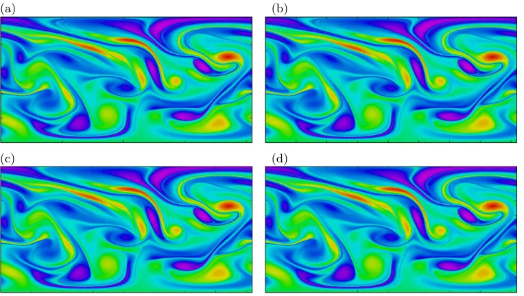
Byt= 400, a further ten times later in the evolution, much of the complex structure evident at t = 40 has cascaded beyond the maximum scale resolved in all simulations — see figure 5 for the two highest resolution GGM and CLAM results. Nonetheless, extensive small-scale structure survives, particularly in the CLAM results. The main four vortices exhibit stepped distributions, ‘vorticity staircases’ (evident also in the GGM results, see below), together with a multitude of small-scale vortices caught between the sharp vorticity gradients. This structure persists, albeit somewhat reduced, all the way to the end of the simulations at t = 4000 (see figure 6). A zoom at t = 4000, shown in figure 7 for the highest resolution CLAM case, reveals the extent of this fine-scale structure — literally hundreds of small-scale vortices exist between the vorticity steps on this large-scale vortex alone. Notably, virtually all of these small-scale vortices have vorticity anomalies which cause the vortices to rotate with the shear associated with the differential rotation of the main large-scale vortex they are embedded in. This gives rise to stabilising ‘cooperative shear’, enabling them to persist for long times, perhaps indefinitely (Dritschel 1990).
(c) (d)
[image:8.595.99.483.102.444.2](e) (f)
Figure 3.Early-intermediate time vorticity distribution ω(r,40), depicted as in figure 2, for
(a) GGM at D = 655362, (b) GGM at D = 2621442, (c) CLAM at ng = 128, (d) CLAM at ng = 256, (e) CLAM at ng = 512 and (f) CLAM at ng = 1024. The percentage decay in enstrophy Z by this time is 56.8%, 52.2%, 50.0%, 44.1%, 38.3% and 32.4%, respectively. In CLAM, the results are plotted on a grid 16 times finer in each direction except in (e) where every other fine grid point is plotted, and in (f) where every 4th grid point is plotted. Same color scale as in Fig. 1.
(a) (b)
0.0 0.5 1.0 1.5 2.0 2.5 3.0 3.5
9 8 7 6 5 4 3 2 1 0
lo
g1
0
Z
log10l
0.0 0.5 1.0 1.5 2.0 2.5 3.0 3.5
6 5 4 3 2 1 0
lo
g1
0
Z
[image:9.595.101.479.103.278.2]log10l
Figure 4.1D vorticity power spectraZ(l, t) at (a) at t= 4 and (b)t= 40. Colours (online) cycle from black, to blue, to red, to green and back to black, starting from the lowest resolution GGM simulation (D= 163842) and ending with the highest resolution CLAM one (ng= 1024). Three spectra are shown for GGM and four are shown for CLAM. The lowest resolution CLAM spectrum is shown in green.
(a) (b)
(c) (d)
Figure 5.Intermediate-late time vorticity distributionω(r,400), depicted as in figure 2 & 3,
for (a) GGM atD= 655362, (b) GGM atD= 2621442, (c) CLAM atng= 512 and (d) CLAM at ng = 1024. Note, only the two highest CLAM results are shown, but the lower resolution results are qualitatively similar. By this time, the enstrophyZ has decayed to approximately 21% of its initial value in all cases. No further significant decay occurs tot= 4000 (<0.05%). Same color scale as in Fig. 1.
once the possibility of encountering another vortex in a nearby streamline at close range has been eliminated.
[image:9.595.100.482.349.561.2](c) (d)
Figure 6.Late (and final) time vorticity distributionω(r,4000), depicted as in figure 2 & 3,
for (a) GGM atD= 655362, (b) GGM atD= 2621442, (c) CLAM atng= 512 and (d) CLAM atng= 1024. Same color scale as in Fig. 1.
representation of the vorticity in GGM removes the small steps due to the CLAM contour level spacing evident in figure 8 but reproduces the larger steps. The stepped vorticity distributions seen here appear to be closely analogous to those arising spontaneously in rotating 2D turbulent flows having a mean ‘planetary’ vorticity gradient (see Dritschel & McIntyre (2008) for a review). There, turbulence cannot entirely break down this gradient but rather mixes vorticity inhomogenously, resulting in a stepped vorticity distribution in the inviscid limit (Scott & Dritschel 2012). The associated flow consists of a series of eastward (prograde) jets centred on each step, reminiscent of the jets observed in many planetary atmospheres, most notably Jupiter’s (Marcus 1993). In the simulations conducted here, each large-scale vortex has a vorticity gradient which is reshaped into a stepped distribution early on in the turbulent flow evolution.
The impact of this turbulent mixing can also be seen in the area fraction occupied by each vorticity level — the so-called ‘vorticity measure’ p(ω, t). This is shown at a few selected times in figure 10 for the highest resolution GGM and CLAM simulations, in (a) and (b) respectively. In a perfectly inviscid fluid,p(ω, t) is time-independent and generates the conserved Casimirs in (2.5) through the relations Cn = 4πRωnp(ω)dω,
n = 2,3, .... The lack of conservation seen here is caused by the inevitable cascade of vorticity to small scales — none of the Casimirs can be preserved in simulations at finite resolution (indeed,C2decays by 79% here). The initial vorticity measurep(ω,0) is broadly
distributed between ωmin = −5.1187 and ωmax = 5.7996, then narrows and diminishes
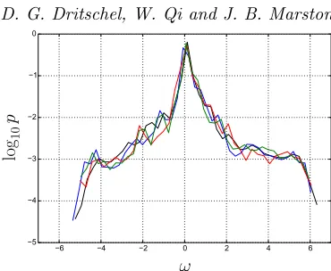
nearly everywhere except for values ofω near 0. By t= 400, the vorticity measure has converged to a nearly fixed form, which is noticeably jagged, perhaps related to the non-monotonic vorticity profiles seen in figure 8(a). At late times, despite the inherently unpredictable nature of the flow evolution, p(ω, t) remains closely similar between the numerical methods and across resolutions, as shown in figure 11. Hence, the vorticity measure is not sensitive to differences in the vorticity dynamics.
In the CLAM results in figure 10(b), notice thatωmin andωmaxare conserved, and that
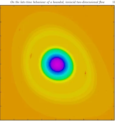
Figure 7.Zoomed, full-resolution view att= 4000 of the vortex seen in the lower-left part of figure 6(d). The view is centred at longitude−15π/16 and latitude−π/8, and shows aπ/2 range in longitudes and latitudes (1/8th of the domain or 81922
grid points). Colours (online) range from the minimum to the maximum vorticity in the domain of view. Concentric steps seen in the vorticity are an artifact of the discretization of the vorticity levels in the CLAM algorithm.
time. This is sensible physically, as the extreme values are most resilient to deformation. On the other hand, in the GGM results, there is clear evidence of hyperviscous overshoot: the extreme values are not conserved (at times not shown here they are nearly twice their initial values). Slightly greater and unphysical extreme values persist to the end of the simulation, though they have very small measure. In both simulations, the observed strong growth ofp(ω, t) nearω= 0 is due to the efficient mixing of weak vorticity, which essentially behaves as a passive scalar. As|ω|increases, it becomes increasingly difficult to shear out vorticity structures and mixing becomes less efficient.
3.2. Unsteadiness
0 1000 2000 3000 4000 5000 6000 7000 8000 6
5
i
0 1000 2000 3000 4000 5000 6000 7000 8000
0 1
i
(c) (d)
0 1000 2000 3000 4000 5000 6000 7000 8000
6 5 4 3 2 1 0
ω
i
0 1000 2000 3000 4000 5000 6000 7000 8000
0 1 2 3 4 5 6
ω
[image:12.595.98.479.105.438.2]i
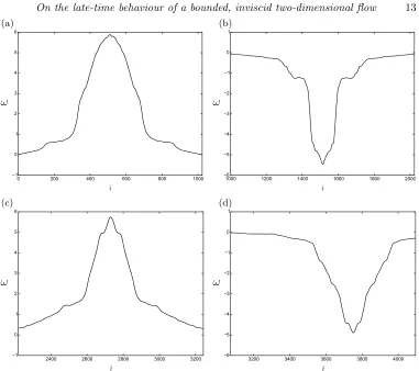
Figure 8.(a)–(d) Constant-latitude cross sections of the vorticity field taken through each of the 4 large-scale vortices (from left to right in figure 6(d)) in the highest resolution CLAM simulation att= 4000. The relative longitudinal grid pointiis indicated on the horizontal axis. The small steps show the vorticity contour level spacing used in the CLAM simulation. The important features are the large steps, seen in many of the vortices. Note also that the cross sections occasionally pass through a small-scale vortex.
(a) (b)
0 200 400 600 800 1000
1 0 1 2 3 4 5 6 ω i
10006 1200 1400 1600 1800 2000
5 4 3 2 1 0 1 ω i (c) (d)
2400 2600 2800 3000 3200
1 0 1 2 3 4 5 6 ω i
3200 3400 3600 3800 4000
[image:13.595.100.481.104.442.2]6 5 4 3 2 1 0 1 ω i
Figure 9.As in figure 8 but for highest resolution GGM simulation att= 4000. Large steps in the vorticity remain evident.
(a) (b)
8 6 4 2 0 2 4 6 8
6 5 4 3 2 1 0 lo g1 0 p ω
8 6 4 2 0 2 4 6 8
6 5 4 3 2 1 0 lo g1 0 p ω
Figure 10. The log-scaled vorticity measure log10p(ω, t) at selected times in (a) the highest
[image:13.595.100.479.480.636.2]6 4 2 0 2 4 6 5
[image:14.595.194.379.103.255.2]ω
Figure 11.Comparison of log10p(ω, t) att= 4000 between the two highest resolution GGM
simulations with (colours online)D = 655362 (black) and D = 2621442 (blue), and the two highest resolution CLAM simulations withng = 512 (red) andng = 1024 (green).
(a) (b)
Figure 12.Scatter plots of vorticityωvs. streamfunctionψ att= 4000 in (a) the highest resolution GGM simulation, and (b) the highest resolution CLAM simulation.
the flow remains unsteady and extremely complex, even despite the inevitable dissipation in CLAM which acts to remove small-scale structure over time (see discussion above).
An alternative way of measuring the unsteadiness of the flow was introduced by Qi & Marston (2014). They developed a rotation and amplitude independent measure of the flow configuration that involves only the streamfunction amplitudes ψℓm of the spheri-cal harmonicsYm
ℓ of degreeℓ= 2 (these coefficients characterise the main quadrupolar pattern seen at late times). The ordermsatisfies −26m62. Using the standard con-vention for spherical harmonics (for whichY−m
ℓ = (−1) mYm∗
ℓ where ∗denotes complex conjugation), the configuration is obtained from the amplitudes:
W(t) = −2 ψ
3
20+ 6ψ20(ψ2,−1ψ21+ 2 ψ2,−2 ψ22)−3
√
6 (ψ2,−2 ψ 2 21+ψ
2
2,−1 ψ22)
ψ2 2,−2+ψ
2 2,−1+ψ
2 20+ψ
2 21+ψ
2 22
32
.
(3.1) W ranges from−2 to +2; when|W|= 2, there are just two vortices, while whenW = 0 there are four of equal intensity. The sign ofW indicates the sign of the dominant pair of same-signed vortices.
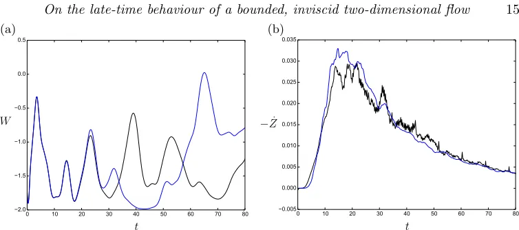
[image:14.595.98.480.307.445.2](a) (b)
0 10 20 30 40 50 60 70 80
2.0 1.5 1.0 0.5 0.0 0.5
W
t
0 10 20 30 40 50 60 70 80
0.005 0.000 0.005 0.010 0.015 0.020 0.025 0.030 0.035
−Z˙
[image:15.595.101.478.104.271.2]t
Figure 13.Early time evolution (06 t6 80) of (a) the ‘configuration’W(t) (defined in the text) and (b) the rate of enstrophy dissipation −dZ/dt=−Z˙, for both the highest-resolution CLAM and GGM simulations. Colours (online) show CLAM in black and GGM in blue.
in (b)). After this time, the results diverge due to the loss of predictability. However, both methods — at all resolutions — exhibit the same qualitative behaviour in W(t) thereafter: quasi-periodic and non-diminishing oscillations, i.e. persistent unsteadiness. This is shown in figure 14 for two very long integrations carried out to aroundt= 10000; the top panel shows GGM atD= 655362 while the bottom shown CLAM atng= 1024 (both fort>200). Movies of the flow evolution indicate that the oscillations are caused by the four main vortices moving around each other, with global-scale excursions, and with no sign of relaxing to equilibrium. Note that similar oscillations are also seen in the dipole case of figure 2 of Morita (2011) where they are described as ‘small perturbations’ without detailed discussion.
A simple model of this vortex motion is to consider just 4 point vortices, singular dis-tributions, in place of the continuous vorticity distribution above. For point vortices, the dynamical system has just 3 degrees of freedom, after taking into account conservation of energy, angular momentum and the fact that the dynamics depends only on the relative (angular) separation of the vortices (Polvani & Dritschel 1993; Newton 2001). The vor-tex motion is therefore either quasi-periodic or chaotic in general; steady configurations are rare (indeed of zero probability for arbitrary choices of the vortex circulations and positions).
To test the effectiveness of this simple model, the 4 main vortices from the highest resolution CLAM simulation att= 4000 (see figures 6 and 8) were identified by locating contiguous vorticity regions having |ω| > 0.2, a small threshold value enabling one to capture most of the circulation within each vortex. The circulations Γk (k= 1,2,3 & 4) were found by area integration over each contiguous region of vorticity Rk, and the centresrk from
rk = 1
Γk
Z Z
Rk
ωrdΩ. (3.2)
This procedure however does not lead to zero angular impulseL, which for point vortices
is equal toP
kΓkrk. SinceL= 0 in the original flow, we adjust the circulations Γk by subtracting λ·rk for each k, whereλ is determined from a 3×3 linear system. This
!0.80
t
1000 2000 3000 4000 5000 6000 7000 8000 9000 10000
W
!0.95
!0.90
!0.85
!0.80
!0.75
!0.70
t
1000 2000 3000 4000 5000 6000 7000 8000 9000 10000
!0.80
!0.75
8500 8600 8700 8800
!0.80
!0.75
[image:16.595.95.477.101.371.2]1400 1500 1600 1700
Figure 14.Late time evolution (t>200) of the ‘configuration’W(t) for both the second highest resolution GGM simulation (top) and highest resolution CLAM simulation (bottom).
0 50 100 150 200
0.95 0.90 0.85 0.80 0.75 0.70 0.65 0.60 0.55
W
t
Figure 15. W(t) over the final 10 periods of evolution (approximately 192 time units) in the CLAM, GGM and point-vortex simulations. Time is shown relative totmax−192 in each simulation. Colours (online) show CLAM in black, GGM in blue, and the point vortex model in red.
With Γk andrk determined in this way, the governing dynamical system drk
dt = 1 4π
4
X
j=1, j6=k Γj
rj×rk
1−rj·rk (k= 1,2,3,4) (3.3)
[image:16.595.197.378.415.553.2]4.0 3.5 3.0 2.5 2.0 1.5 1.0 0.5 10
8 6 4 2 0
lo
g
10W
4.0 3.5 3.0 2.5 2.0 1.5 1.0 0.5
10 8 6 4 2 0
lo
g
10W
4.0 3.5 3.0 2.5 2.0 1.5 1.0 0.5
10 8 6 4 2 0
lo
g
10W
[image:17.595.98.476.105.390.2]log
10f
Figure 16.Configuration frequency spectrum W(f) for the second highest resolution GGM simulation (top), the highest resolution CLAM simulation (middle), and the point vortices (bot-tom). In GGM,W(f) was computed from the time series ofW fort∈[400,10000]; in CLAM we used [400,9022], while in the point-vortex model we used [0,4000].
simulations is shown in figure 15. (The averages and amplitudes ofW(t) differ slightly due to the largely unpredictable nature of turbulence and the crude fitting method of the point-vortex system.) Much longer point-vortex simulations carried out to t = 106
exhibit the same behaviour, with undiminished oscillations.
The correspondence between the three simulations is even more remarkable if one examines the frequency power spectrum of W, namely W(f) = |Wˆ|2
, where ˆW is the Fourier transform ofW and f is the frequency (here equal to the inverse period). The frequency spectra (log10scaled) for the three simulations are shown in figure 16, vertically
aligned, with GGM on top, CLAM in the middle, and the point vortices on the bottom. Most strikingly, the dominant frequency f = 1/T with T ≈ 19.14 is matched in all three simulations. The power at this frequency is orders of magnitude above surrounding frequencies, indicating that the dynamics are very nearly periodic. Other less prominent peaks also line up, corresponding to longer period oscillations. Overall, the agreement is remarkable, given the enormous simplifications made to reduce the dynamics to that of 4 point vortices. Most importantly, the point vortex model strongly supports our claim that the dynamics never comes to equilibrium.
4. Conclusions
be-native. At long times, the vorticity field is primarily concentrated in 4 large vortices. They are generally unequal in circulation, and not regularly spaced. If one replaces each vortex by a point vortex of the same circulation, we have shown that the point vortices typically exhibit unsteady quasi-periodic motion — persistent unsteadiness. Fundamen-tally, we argue, the observed unsteadiness in the Euler equations for continuous vorticity is intimately associated with the unsteadiness of 4 point vortices moving on the surface of a sphere.
We have also found that small-scale vortices pepper the flow field at high resolution. These vortices commonly have vorticity anomalies which cause the vortices to rotate in the same sense as the shear induced by differential rotation of the main vortex they circulate about. The small-scale vortices therefore experience a stabilising cooperative shear (Dritschel 1990). As a result, even these small-scale vortices may persist indefinitely. Moreover, as the resolution increases, more structure at small scales appear. Our main conclusion is that bounded inviscid flows on a sphere, with zero angular momentum, typically do not settle down to an equilibrium; instead, a few robust compact vortices emerge from the early flow evolution and interact chaotically or quasi-periodically.
In the much studied case of doubly-periodic geometry, by contrast, often two opposite-signed vortices emerge. In this case, the corresponding point-vortex system is integrable, and the only possible motion is simple steady translation. This difference from spherical geometry greatly facilitates the emergence of a steady flow (in a translating frame of reference), though one still cannot rule out the persistence of small-scale vortices circu-lating around the main large-scale vortices. Inviscid flows in a doubly-periodic domain are likely to be less unsteady than flows on a sphere, though unsteadiness may persist forever.
We are grateful for helpful discussions with Freddy Bouchet, James Cho, Bruce Turk-ington, Antoine Venaille, and Peter Weichman. We thank the Kavli Institute for Theoret-ical Physics for supporting our participation in the 2014 Program “Wave-Flow Interaction in Geophysics, Climate, Astrophysics, and Plasmas” where this work was initiated. The KITP is supported in part by the NSF Grant No. NSF PHY11-25915. This work was also supported in part by the NSF under grant Nos. DMR-1306806 and CCF-1048701 (JBM and WQ).
Appendix A. Initial Condition
The initial streamfunction at timet= 0 is a superposition of spherical harmonics with spherical wavenumber in the range 46ℓ610,
ψ(θ, φ) =
10
X
ℓ=4 ℓ
X
m=−ℓ
withψℓ−m= (−1)mψℓm∗ and the following choice of amplitudesψℓm:
ψ40=−0.0114727
ψ41= 0.0255012 + 0.0337679i
ψ42=−0.0366116−0.0312419 i
ψ43= 0.000614585 + 0.000602384i
ψ44= 0.0160784−0.0194655i
ψ50= 0.00357198
ψ51=−0.000446705−0.0100286i
ψ52= 0.0100984 + 0.00778139i
ψ53=−0.0142904−0.00864324i
ψ54= 0.0156104−0.0111872 i
ψ55=−0.00275238−0.0106832 i
ψ60=−0.00352493
ψ61=−0.00739953 + 0.00218422i
ψ62= 0.0140976 + 0.00864871i
ψ63=−0.0141289−0.00654953i
ψ64= 0.0200989−0.0152088 i
ψ65= 0.00682398 + 0.0132045i
ψ66= 0.00919374 + 0.00889445i
ψ70= 0.00269739
ψ71=−0.00607359−0.00179029i
ψ72= 0.00299202−0.0115332i
ψ73=−0.00418447−0.000665072i
ψ74= 0.00853673−0.0011805i
ψ75=−0.00229449−0.00731682i
ψ76= 0.00315312−0.00332254i
ψ77= 0.0127047 + 0.000153664i
ψ80=−0.0070908
ψ81=−0.00820113−0.00180399i
ψ82= 0.00726466−0.00109238i
ψ83= 0.00327615 + 0.00732665i
ψ84=−0.00418371 + 0.00764604i
ψ85=−0.00506492 + 0.00152613i
ψ86= 0.00289222−0.0126644i
ψ87=−0.00113653−0.00983086i
ψ88= 0.00390903 + 0.00337946i
ψ98=−0.00309726−0.000427295i
ψ99=−0.0053439 + 0.00203709i
ψ100=−0.00507863
ψ101=−0.00247735 + 0.00024564i
ψ102=−0.00357194−0.00141963i
ψ103=−0.00077508 + 0.00719427i
ψ104=−0.00462811−0.00550109i
ψ105=−0.00101044−0.00773111i
ψ106= 0.00395564 + 0.0027653i
ψ107= 0.00121852 + 0.00310834i
ψ108= 0.00314655 + 0.000289766i
ψ109=−0.00279021−0.00314691i
ψ1010= 0.00258861−0.000254598i (A 2)
REFERENCES
Abramov, R. V. & Majda, A. J.2003 Statistically relevant conserved quantities for truncated quasigeostrophic flow.Proc. Natl. Acad. Sci.100, 3841–3846.
Bouchet, F. & Corvellec, M.2010 Invariant measures of the 2D Euler and Vlasov equations.
J. Stat. Phys.: Theor. Expt.2010, P08021.
Bouchet, F. & Venaille, A.2012 Statistical mechanics of two-dimensional and geophysical flows.Phys. Rep.515, 227–295.
Brands, H., Stulemeyer, J., Pasmanter, R. A. & Schep, T. J.1997 A mean field prediction of the asymptotic state of decaying 2D turbulence.Phys. Fluids 9, 2815–2817.
Bricmont, J., Kupiainen, A. & Lefevere, R.2001 Ergodicity of the 2D Navier-Stokes equa-tions with random forcing.Comm. Math. Phys.224, 65–81.
Charney, J.1949 On a physical basis for numerical prediction of large-scale motions in the atmosphere.J. Meteor. 6, 371–385.
Chavanis, P. H. 2002Dynamics and Thermodynamics of Systems with Long-Range Interac-tions.,Lecture Notes in Physics, vol. 602, pp. 208–289. Springer, Berlin Heidelberg.
Chavanis, P. H. 2009 Dynamical and thermodynamical stability of two-dimensional flows: variational principles and relaxation equations.Euro. Phys. J. B 70, 73–105.
Dritschel, D. G.1988 Contour surgery: a topological reconnection scheme for extended inte-grations using contour dynamics.J. Comput. Phys.77, 240–266.
Dritschel, D. G.1990 The stability of elliptical vortices in an external straining flow.J. Fluid Mech.210, 223–261.
Dritschel, D. G. & Fontane, J.2010 The combined Lagrangian advection method.J. Com-put. Phys.229, 5408–5417.
Dritschel, D. G., Haynes, P. H., Juckes, M. N. & Shepherd, T. G.1991 The stability of a two-dimensional vorticity filament under uniform strain.J. Fluid Mech.230, 647–665.
Dritschel, D. G. & McIntyre, M. E.2008 Multiple jets as PV staircases: the Phillips effect and the resilience of eddy-transport barriers.J. Atmos. Sci 65, 855–874.
Dritschel, D. G. & Scott, R. K.2009 On the simulation of nearly inviscid two-dimensional turbulence.J. Comput. Phys.228, 2707–2711.
Dritschel, D. G., Scott, R. K., Macaskill, C., Gottwald, G. A. & Tran, C. V.2009 Late time evolution of unforced inviscid two-dimensional turbulence.J. Fluid Mech.640, 215–233.
Dritschel, D. G. & Tobias, S. M.2012 Two-dimensional magnetohydrodynamic turbulence in the small Prandtl number limit.J. Fluid Mech.703, 85–98.
Dritschel, D. G., de la Torre Ju´arez, M. & Ambaum, M. H. P.1999 On the three-dimensional vortical nature of atmospheric and oceanic flows.Phys. Fluids 11, 1512–1520.
Dritschel, D. G., Tran, C. V. & Scott, R. K.2007 Revisiting Batchelor’s theory of two-dimensional turbulence.J. Fluid Mech.591, 379–391.
Dubinkina, S. & Frank, J.2010 Statistical relevance of vorticity conservation in the Hamil-tonian particle-mesh method.J. Comput. Phys.229, 2634–2648.
Eyink, G. L. & Sreenivasan, K. R.2006 Onsager and the theory of hydrodynamic turbulence.
Rev. Mod. Phys.78, 87–135.
Fjørtoft, R.1953 On the changes in the spectral distribution of kinetic energy for twodimen-sional, nondivergent flow.Tellus 5, 225–230.
Fontane, J. & Dritschel, D. G. 2009 The HyperCASL Algorithm: a new approach to the numerical simulation of geophysical flows.J. Comput. Phys.228, 6411–6425.
Heikes, R. & Randall, D. A.1995a Numerical integration of the shallow-water equations on a twisted icosahedral grid. Part I. Basic design and results of tests.Mon. Wea. Rev.123, 1862–1880.
Heikes, R. & Randall, D. A.1995bNumerical integration of the shallow-water equations on a twisted icosahedral grid. Part II. A detailed description of the grid and an analysis of numerical accuracy.Mon. Wea. Rev.123, 1881–1887.
Herbert, C.2013 Additional Invariants and Statistical Equilibria for the 2D Euler Equations on a Spherical Domain.J. Stat. Phys.152, 1084–1114.
Jim´enez, J.1994 Hyperviscous vortices.J. Fluid Mech.279, 169–176.
Majda, A. J. & Wang, X.2006Nonlinear Dynamics and Statistical Theories for Basic Geo-physical Flows.. Cambridge University Press.
Marcus, P. S.1993 Jupiter’s great red spot and other vortices.Annu. Rev. Astron. Astrophys.
31, 523–573.
Mariotti, A., Legras, B. & Dritschel, D. G. 1994 Vortex stripping and the erosion of coherent structures in two-dimensional flows.J. Fluid Mech.6, 3954–3962.
Matthaeus, W. H., Stribling, W. T., Martinez, D., Oughton, S. & Montgomery, D.
1991a Decaying, two-dimensional, Navier-Stokes turbulence at very long times.Physica D: Nonlin. Phenomena51, 531–538.
Matthaeus, W. H., Stribling, W. T., Martinez, D., Oughton, S. & Montgomery, D.
1991b Selective decay and coherent vortices in two-dimensional incompressible turbulence.
Phys. Rev. Lett.66, 2731–2734.
Miller, J.1990 Statistical mechanics of Euler equations in two dimensions.Phys. Rev. Lett.
65, 2137–2140.
Miller, J., Weichman, P. B. & Cross, M. C.1992 Statistical mechanics, Euler’s equation, and Jupiter’s Red Spot.Phys. Rev. A45, 2328–2359.
Mohebalhojeh, A. R. & Dritschel, D. G.2007 Assessing the numerical accuracy of complex spherical shallow water flows.Mon. Wea. Rev.135, 3876–3894.
Montgomery, D., Matthaeus, W. H., Stribling, W. T., Martinez, D. & Oughton, S.
1992 Relaxation in two dimensions and the ”Sinh-Poisson” equation.Phys. Fluids A 4, 3–6.
Robert, R. & Sommeria, J. 1991 Statistical equilibrium states for two-dimensional flows.
J. Fluid Mech.229, 291–310.
Scott, R. K. & Dritschel, D. G.2012 The structure of zonal jets in geostrophic turbulence.
J. Fluid Mech.711, 576–598.
Segre, E. & Kida, S.1998 Late states of incompressible 2d decaying vorticity fields. Fluid Dynamics Research23, 89–112.
Whitaker, Nathaniel & Turkington, Bruce1994 Maximum entropy states for rotating vortex patches.Physics of Fluids 6(12), 3963.
Williams, P. D. 2009 A proposed modification to the Robert-Asselin time filter.
Mon. Wea. Rev.137, 2538–2546.
Yao, H. B., Dritschel, D. G. & Zabusky, N. J. 1995 High-gradient phenomena in two-dimensional vortex interactions.Phys. Fluids 7, 539–548.
Yin, Z., Montgomery, D. C. & Clercx, H. J. H. 2003 Alternative statistical-mechanical descriptions of decaying two-dimensional turbulence in terms of “patches” and “points”.
Physics of Fluids 15, 1937–1953.