A Simple Predictive Performance Model of Solar Cell under Very Hot and Humide Climate

(1)

ISSN Online: 2327-5901 ISSN Print: 2327-588X

DOI: 10.4236/jpee.2019.75004 May 27, 2019 26 Journal of Power and Energy Engineering

A Simple Predictive Performance Model of

Solar Cell under Very Hot and Humide Climate

Mougang Yolande Christelle Ketchanji

*

, Essiane Salomé Ndjakomo, Imano Adolphe Moukengue

Laboratory Technology and Applied Sciences, University of Douala, Douala, Cameroon

Abstract

In the scope of solar energy-based electrical needs in rural tropical regions, the present article develops and confronts experimental power models from the using of manufacturer data and a new model made with the meteorologi-cal and electrimeteorologi-cal data acquired. These data are registered through an acquisi-tion staacquisi-tion around a monocrystalline photovoltaic panel, designed and rea-lized in the scope of this work. After the acquisition of meteorological data, a choice of the most relevant meteorological variable as input vectors to express the output powers obtained was carried out. Around the Single-Diode model, seven models are performed with analytics equations, iterative methods and an optimization method with a multi-objective function to get internal para-meters. The proposed experimental model is made by a combination of the solution got at STC of an iterative method, with the value of nameplate and the use of an open circuit voltage equation with experimental coefficient to predict power output in operating conditions, and it’s demonstrated more ef-ficient. The optimization of a multi-objective function using Nonlinear Squares (NLS) through the Leveng-Marqued method to solve the parameter estima-tion of a PV panel has been well done and the results are useful, like classic iterative method and less time-consuming.

Keywords

Experimental, Modelling, Maximal Power Output (MPO), Photovoltaic (PV), 1M5P

1. Introduction

Around 84% of 1.5 billion people without electricity access reside in rural areas and more than 95% of those living without electricity are in countries in sub-Saharan Africa and developing Asia [1]. In rural areas, more than 1.5 billion people lack How to cite this paper: Ketchanji, M.Y.C.,

Ndjakomo, E.S. and Moukengue, I.A. (2019) A Simple Predictive Performance Model of Solar Cell under Very Hot and Humide Climate. Journal of Power and Energy Engi-neering, 7, 26-47.

https://doi.org/10.4236/jpee.2019.75004

Received: April 26, 2019 Accepted: May 24, 2019 Published: May 27, 2019

http://creativecommons.org/licenses/by/4.0/

(2)

DOI: 10.4236/jpee.2019.75004 27 Journal of Power and Energy Engineering

access to electricity scattered settlements, and hard-to-reach areas. Especially in Cameroon where only 21.7% of rural areas were electrified in 2016, due to a fra-gile economy, costly infrastructure, disseminated habitation and impassable roads. However, the balance of primary energy sources shows a huge dominance of renewable energies: The available hydraulic power is 13.7 GW, and the aver-age irradiance is 4.9 kWh/day/m2_{in the case of Cameroon}_[2]_{. Thus, to} decen-tralize the electrical production and use renewable energies considering their seasonal availability is a huge and urgent challenge. To answer it, a good and realistic modelling of constitutive elements of a power plant is primordial. The aim of this work is to build a robust model to predict electrical power behavior along a day from experimental data for the most present PV module on the rural market. Another scope is to fill the lack of important electrical value for model-ling of a solar panel, not provided by manufacturer like I-V and P-V curves on their datasheet, or not accurate like temperature coefficients, because the usual market panels are not tested under tropical climate conditions. This work leads to evaluate in opposition to usual literature models, the real efficiency of the PV module under meteorological conditions of an equatorial tropical climate.

In this perspective, this work deals with the acquisition of meteorological data and their impact on power output module. Then the confrontation of different mathematical single diode models with manufacturer’s parameters, through models with experimental data from the monocrystalline silicon module LW-MS50 will be performed. Finally, a comparison of different power output pattern based on meteorological data is highlighted.

2. State of Art

The future of the photovoltaic industry is encouraged as the efficiency of the cell and submodules continues to increase [3]. However, the design and optimiza-tion of the photovoltaic system is a difficult step because of the influence of weather conditions on the characteristics and performance of the PV module

[4].

Several studies have been done on the variation in efficiency using different PV technologies [5] [6]. It turns out that the meteorological factors individually influence the models and the performance of all components of the PV module.

Also, the literature review presents some basic knowledge about the modeling PV modules [7] [8]. Models using constant parameters have been proposed [9]

but these models are inaccurate because they don’t take into account the tem-perature variation. In this decade, we develop unique exponential models that neglect shunt resistance [10] [11]. Also, the researchers proposed models consi-dering the temperature and irradiance proposed in the technical sheet [12].

However, despite the existence of numerous mathematical models and soft-ware applications for photovoltaics, sizing is only suitable for the non-tropical regions where they are built [13].

(3)

varia-DOI: 10.4236/jpee.2019.75004 28 Journal of Power and Energy Engineering

tions according to the meteorological conditions, this work after presented the acquisition station, underline in first, the main factors of power variation, then the estimate of this power through mathematical modeling combining various literature approaches for obtaining I-V and P-V characteristics and finally a comparison of power output models with ours and experimental data will be performed.

3. Principle, Data Acquisition and Variations

3.1. Acquisition Station

Few works compare different PV panels or different algorithms at real operating conditions with simulations, or only with experimental evaluation, because it is difficult to find or wait for the same environmental conditions during the expe-rimental tests. Very high costs and feasibilities’ conditions in developing coun-tries limit the use of artificial sun instrument. It is very well known that the de-scription of current-voltage (I-V) and power-voltage (P-V) in different envi-ronmental conditions can characterize a solar cell. However, some common commercial PV panels in rural area don’t present this information and the knowledge of these curves is not enough to estimate the actual generated power of the panels in operating condition. Therefore, an experimental testing system is necessary to have the capability and the reproducibility in environmental con-ditions for comparing several algorithms and characterizing panel.

At this day, it’s not possible to get locally solar irradiation information’s in Douala town, so designing an acquisition station for potential energy estimation needs was paramount. The climatic magnitudes are acquired by three sensors that convert them into electrical signals to be interpreted by the computing and processing which is a Mega Arduino module. Two other sensors of electrical quantities are installed at the output of the photovoltaic module. The five sen-sors implemented are:

• _{Current sensor (ACS712-5A)}

• _{Voltage divider bridge (1/5 resistors of 10 KΩ)} • _{Temperature and humidity (DHT22)}

• _{Wind speed (Adafruit Anemometer 1733)} • _{Irradiation (Apogee pyrometer SP-110)}

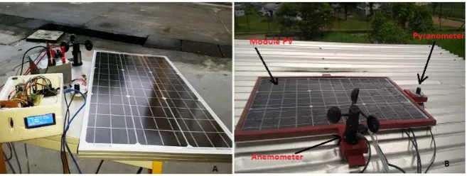
The output power is also calculated after measuring the voltage and current of the panel. These values are displayed on a 20 × 4 LCD for viewing. The same measured values are stored in a 4GB memory card as a text file, which will be imported into the MATLAB software for processing. An overview during the tests carried out at the University Institute of Technology (UIT) of Douala (coordinates are: 4˚05'57,987''N; 9˚74'33,117''E) before and after fixing on a roof is presented in Figure 1.

Consequently, the acquired acquisition station makes it possible to obtain variations in electrical and meteorological quantities such as those observed in

(4)

[image:4.595.210.539.70.194.2]

[image:4.595.210.536.237.411.2]

Figure 1. Acquisition station during the test (A) and after deployment (B) PV module, irradiation sensor, wind speed—UIT of Douala.

Figure 2. Physical quantities measured for a typical day (August-most unfavorable month).

The validation of the acquisition is verified. The temporal data acquired with a fixed resistive load allow obtaining the power according to the output voltage (P

= k × U2_{). Polynomial recognition results in}_k_{= 0.2107 (at 95% confidence} bounds) either: Rmeasured = 4.746 Ω. The relative error of our measurement can then be appreciated: ± 0.97%.

Figure 2 presents a range of humidity between 85% - 99%. For one year of acquisition, the humidity value across a day is usually so high in the region, even if the temperature is at his highest value. Thus, the acquisition reveals that the humidity undoubtedly very high varies slightly but inversely with the tempera-ture.

Hypotheses such as the increase of the power with the irradiation, and the in-crease of temperature of the cells creating an undesirable effect on the electrical efficiency [16] of the panel are verified after the acquisition.

3.2. Relationship between PV Power Output and Environmental

Values

(5)

meteorological parameters and PV power output will not be the same in differ-ent locations. However, the performance of a model is very dependdiffer-ent on the correlation between the input and output values of the model.

Not only solar irradiation is an input parameter, but also other weather para-meters, including atmospheric temperature, module temperature, wind speed and direction, and humidity, are considered as potential parameters for estimat-ing the PV power output [17].

In this case, the study of the correlation of the dissimilar meteorological in-puts, such as solar irradiance, atmospheric temperature, module temperature, wind speed and direction, and humidity, with PV power output, is important. The correlation might be positive or negative. The strongly correlated input va-riables should be used as an input vector to improve the model, and the weakly correlated input vector data should be declined.

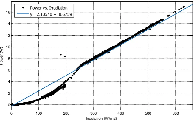
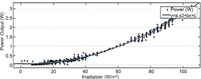
The global solar horizontal irradiance and PV power output of a typical day can be correlated. In a clear-sky day means a normal day, the PV power output is strongly harmonized with the solar irradiance curve. Therefore, a similar pat-tern is observed for PV power output and solar irradiance in any weather condi-tion. Figure 3 shows the high positive correlation between solar irradiance and PV power output in weak solar condition. Like hypothesis, the PV power output is not highly strongly correlated with the solar irradiance on an abnormal day, like a cloudy or rainy day [17]. However, it is strongly matched in Figure 4. So, solar irradiance is an important input vector [18] in evolving an appropriate PV power model due to its high correlation.

[image:5.595.211.537.505.706.2]

Concerning the temperature factor, in the period of the absence of daylight, the PV power output is absent, and no impact of atmospheric temperature exists on the PV power [17]. Thus, atmospheric temperature form variation through-out the day follows the PV power only during the daylight period.

Figure 5 shows the relationship between the atmospheric temperature and the

Figure 3. Power output variation with solar irradiation (R2_{= 0.9616) from data acquisition.}

0 100 200 300 400 500 600

0 2 4 6 8 10 12 14 16

Irradiation (W/m2)

P

ow

er (W

)

(6)

[image:6.595.210.536.70.199.2]

[image:6.595.213.537.245.445.2]

Figure 4. Power output variation with solar irradiation in cloudy conditions (Polynomial of 2nd_{degree R}2_{= 0.9941).}

Figure 5. Power output variation with temperature from data acquisition.

PV power output. The correlation is not high, like for the irradiance input, but not so low.

Therefore, the atmospheric temperature can be used as a significant input to find the projecting model of the PV power output.

The other meteorological quantities measured and recorded by the system (wind speed, humidity) also affect the performance of the solar panel. For rea-sons of calculation speed and exploration space, these quantities will not be tak-en as input vectors in the models of this paper. But will serve to interpret this ending work and can be used to reanalyze models if they are introduced in other upcoming works.

4. Modeling of LW-MS50 and Simulations

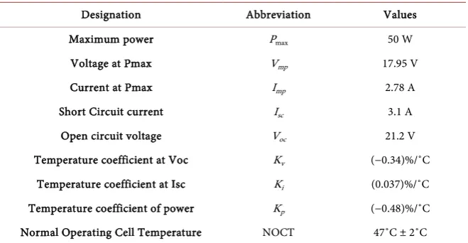
As this work is carried out for a technical-economical optimization for the rural areas of the tropical country, the PV chosen module, for its availability and his low cost on the market, is the LW-MS50. Table 1 presents the characteristics of the nameplate.

25 26 27 28 29 30 31

0 2 4 6 8 10 12 14 16

Temperature (°C)

P

ow

er

'W

)

(7)

[image:7.595.210.540.88.259.2]

Table 1. Characteristics of panel LW-MS50.

Designation Abbreviation Values

Maximum power Pmax 50 W

Voltage at Pmax Vmp 17.95 V

Current at Pmax Imp 2.78 A

Short Circuit current Isc 3.1 A

Open circuit voltage Voc 21.2 V

Temperature coefficient at Voc Kv (−0.34)%/˚C

Temperature coefficient at Isc Ki (0.037)%/˚C

Temperature coefficient of power Kp (−0.48)%/˚C

Normal Operating Cell Temperature NOCT 47˚C ± 2˚C

4.1. Modeling the Photovoltaic Module

Predicting the behavior of I-V and P-V curves for photovoltaic (PV) generation is possible through mathematical models for photovoltaic cells. Several physi-cians have proposed more evolutionary models that present better accuracy for different purposes [9] [19] [20] articles proposed one extra diode to represent the effect of the recombination of carriers. [14] used a model with a current ge-nerator and two diodes in parallel. [21] proposed a three-diode model to include the influence of effects which are not considered by the previous models.

However, a model with a single diode offers a good compromise between simplicity and accuracy [22] and this model is widely used [23]. Sometimes bas-ically or with other components, but always with the basic structure of a current source and a diode in parallel. The usefulness of the single-diode model with a method for adjusting the parameters, and considering experimental data is pro-posed in this paper to really perform this model.

Three equivalent circuit models can be used to describe a single-diode model

[24].

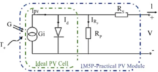
The first is the ideal solar cell, also called 1M3P model (Single Mechanism, Three Parameters). It is an ideal model (Figure 6), where the solar cell can be simply modeled by a p-n junction in parallel with a current source that is asso-ciated to the photocarriers generated.

By adding a series resistance, the model will be close to the real module beha-vior. This proposition is known as the 1M4P model (Single Mechanism, Four Parameters), takes into account the influence of contacts by means of a series re-sistance RS. The Rs resistance is the sum of several structural resistances of the device. In fact, it is proportional to the number of solar cells in the panel [25]. The unknown parameters of this model are: IPV, IS, a and RS.

(8)

[image:8.595.244.506.71.191.2]

Figure 6. Electrical model of solar module.

current of the p-n junction and depends on the fabrication method of the pho-tovoltaic cell. This model has five parameters: IPV, Io, a, RS, RSh, are linked by Eq-uation (1).

e 1

s s t

V R I

a N V s

pv o

p

V R I

I I I

R

 + 

 

 _∗ _∗ 

 

  ₊ _∗

 

= − − −

 

 

(1)

with: Ipv and Is like photovoltaic and saturation currents of the module; Vt =

kT/q: the thermal voltage of the module; Ns cells connected in series; a: diode ideality constant.

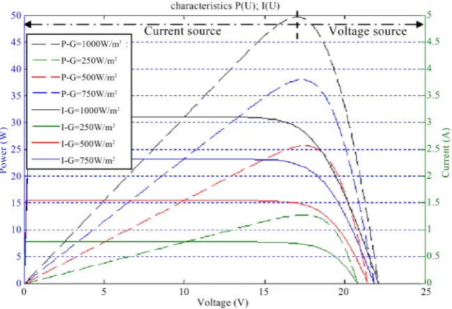
The practical photovoltaic device presents a hybrid behaviour, which may be of current or voltage source depending on the operating point, as shown in Fig-ure 7. There is a series resistance Rs whose impact more when the PV module functions in the voltage source region, and a parallel resistance Rp with stronger influence in the current source region of operation.

The value of Rp is generally high and some authors [26] [27] neglect this re-sistance to simplify the model. The value of Rs is very low and sometimes this parameter is also neglected [28]. So, we will develop in first a model with manu-facturer parameters and without Rp (1M4P).

4.1.1. Model 1M4P

As above announced, four parameters should be found:

• _{It is difficult to determine light-generated current (}_I_pv_{) of the elementary}

cells, without the series and parallel resistances. Datasheets only notify on the nominal short-circuit current (Isc,n), which is the maximum current available at the PV module output. The hypothesis Isc ≈ Ipv is frequently used in pho-tovoltaic models. In fact, the series resistance is less than 1 Ω, and the parallel resistance is more than 100 Ω in practical devices. Without temperature in-fluence [29] provides Equation (2) where Ipv depends on real irradiance (G):

pv sc

o

G

I I

G

= × ₍₂₎

• _{It’s considering that our solar cell is like a luminescent diode, to obtain}_I_o_.

(9)

[image:9.595.212.537.72.294.2]

Figure 7. Power and current-voltage characteristics-1M4P.

ln cc 1

oc t

s I

V V

I

  = × _ + _

  (3)

In this way, we obtain:

exp 1

cc o

co

s t

I I

V N V

=

 

−

 _∗ 

 

(4)

The Equation (4) in Equation (1) at the maximum power point gives us: 1

ln

sc mp

mp o

s s t

mp mp

I I

V I

R aN V

I I

 −  +  

 

 

= × _ _−

 

 

(5)

These previous equations lead to get characteristic curves of I-V and P-V like shown in Figure 7.

To show the effect of irradiance on the performance of a module, the temper-ature is kept fixed at 25˚C and the values of irradiance are changed to different values. The variation of the I(V) characteristics with irradiance is shown in Fig-ure 7. Irradiance has the principal effect on the short circuit current and indeed the relationship between irradiance and the short circuit current is a linear one in this model. The simulations lead to the validation of the model according to

Figure 7, when the irradiation decreases, the maximum power decreases also.

4.1.2. Cell Currents with Classic Temperature Adjustments

(10)

(

,

)

pv pv n i T

n

G

I I K

G

∆

= + ₍₆₎ where: Ipv,n [A] is the light-generated current at the nominal condition (usually 25˚C and 1000 W/m2_),

T T Tn

∆ = − _(being_T_and_T_n_{the actual and nominal} temperatures of cell [K]), G [W/m2_{] is the irradiation on the device surface, and}

Gn is the nominal irradiation.

The saturation current I0 of the photovoltaic cells that compose the device de-pends on the saturation current density of the semiconductor (Jo, generally given in [A/cm2_{]) and on the effective area of the cells}_[31]_.

3

0 0,n n exp g 1 1

n

qE T

I I

T ak T T

  

 

= _ _ _ _ − __

     (7) where Eg is the bandgap energy of the semiconductor (Eg ≈ 1.12 eV for the poly-crystalline-Si at 25˚C), and I0,n is the nominal saturation current as:

, 0, , exp 1 SC n n OC n s t I I V aN V =   −     (8)

The values of Eg, and Jo are infrequently available for commercial photovoltaic arrays. In the following, the nominal saturation current I0,n is indirectly obtained from the experimental data through Equation (8), which is obtained by evaluat-ing Equation (1) at the nominal open-circuit condition, with V = Voc,n, I = 0, and

Ipv≈ Isc,n.

The photovoltaic model described in the previous section can be improved with temperature coefficients.

The saturation current I0 is strongly dependent on the temperature and we propose a different approach to express the dependence of I0 on the temperature. We obtained the Equation (9) from (8) by including in the equation the current and voltage coefficients Ki and Kv.

, 0

,

exp 1

SC n i T

OC n V T

t I K I V K aV + = +   −  ∆   

∆ (9)

This equation withdraws the model error at the vicinities of the open-circuit voltage point and consequently at other regions of the I-V curves and will simpl-ify the model.

The realism of this equation has been tested with all three single-diode models by simulation.

(11)

The value of the diode constant n will be arbitrarily chosen. Many authors discuss ways to estimate the correct value of this constant [22]-[32]. Usually, 1 ≤

a ≤ 1.5 and the choice depends on other parameters of the I-V model. Some val-ues for n are found in [30] based on empirical analysis. As [22] says, there are different opinions about the best way to choose a. In fact, the value n is totally empirical, and an initial value of a can be chosen in order to improve the model. The value of n can be later modified to improve the model fitting if necessary.

4.1.3. Model 1M5P: RS, Rp and a Values Solved by Iterative Methods

Equation (1) does not have a direct solution because: I g V I=

(

,

)

and

(

,

)

V = f I V . This transcendental equation can be solved by a numerical method. The I-V points are easily obtained by numerically solving

(

,

)

(

,

)

0

g V I = −I f V I =

for a set of V values and obtaining the corresponding set of I points. And the couple (Rs, Rp) is still unknowing.

Rs and Rp may not be solved separately if we are looking for a realist I-V mod-el. Rp can be found if we have a value of Rs.

To reach these values, methods in the literature, and the proposed method are run out.

1) Villalva’s Method

This described method [33] allows only finding Rs and thus Rp using the point of maximum power. Not only with the I-Vcurve but also with the P-V (power vs. voltage) curve, which must match the experimental data too.

The target is to find the value of Rs (and later Rp) that the highest value of the P-V curve coincides with the experimental peak power at the (Vmp, Imp) point. This requires several iterations until Pmax,m = Pmax,e.

Just the peak power value is required, and the iterative process incremented Rs starting from zero and adjusting the P-V curve to match the experimental data. Plotting the P-V and I-V curves require solving Equation (1) on the interval

, , 0 0 sc n oc n I I V V ≤ ≤   ≤ ≤  .

Subsequently, different values of a can be explored to improve the model fit-ting. In fact, this constant affects the I-V characteristic and his variation mod-ifies the precision of this curve [33].

The Equation (6) and Equation (9) are used to obtain Ipv and Io, and by consi-dering that Ipv,n is giving by Equation (10):

(

)

, ,

sc n s p

pv n

p

I R R

I

R

+

= ₍₁₀₎ Equation (10) is written at the maximum power point of Equation (1)

(

)

(

)

0 exp 0 max,

mp mp S mp

p

mp mp S

mp PV mp mp e

S

V V R I

R

V I R

q

V I V I V I P

(12)

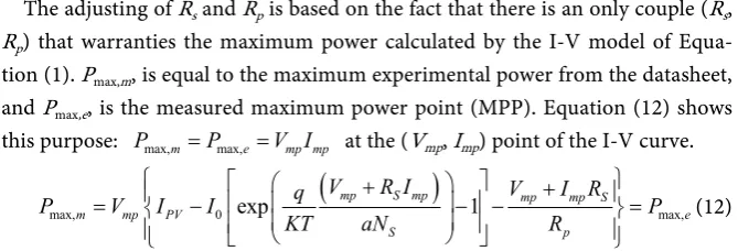
The adjusting of Rs and Rp is based on the fact that there is an only couple (Rs,

Rp) that warranties the maximum power calculated by the I-V model of Equa-tion (1). Pmax,m, is equal to the maximum experimental power from the datasheet, and Pmax,e, is the measured maximum power point (MPP). Equation (12) shows this purpose: Pmax,m =Pmax,e=V Imp mp at the (Vmp, Imp) point of the I-V curve.

(

)

max, 0 exp 1 max,

mp S mp mp mp S

m mp PV e

S p

V R I V I R

q

P V I I P

KT aN R

   +   + 

 _ _ _ _ 

= _ − − − _=

 

 

 _ _ _ _ 

 

[image:12.595.206.541.76.190.2]

(12)

Figure 8 illustrates how this iterative process works when Rs increases, the P-V curve moves to the left and the peak power (Pmax,m) goes towards the expe-rimental MPP.

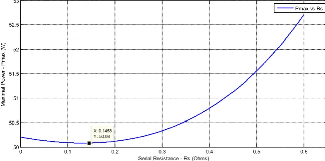
Also the same concept for graphically finding the solution for Rs is performed. For each fixed Rs, the curve P(V) is plotted by varying V from 0 to Voc. Accor-dingly, for each series of P(V, Rs), a higher value result. We can then draw the curve of the maximum values of P(V) corresponding to each Rs. The minimum of this curve corresponds to Pmax,e and to the value of Rs sought. Figure 9 shows a plot of Pmax,m as a function of Rs.

At this stage of work, P(V) and I(V) curve are also adjusted to three remarka-ble points for V = 0, Vmp, and Voc.

2) Modified Newton-Raphson Method

This iterative method is common to find the root of a function f(Rs). A value of Rs is chosen and incremented until the stop condition isn’t obtained. If the value of f(Rs) divided by its derived function is less than the tolerance value, then the value of Rs is retained and Rp, with the other values are computed. Another test cycle can be used to explore different values of the coefficient a. Interval 1 ≤

[image:12.595.211.538.521.707.2]

a ≤ 1.5, is usually used [33].

Figure 10 presents the applied algorithm. The algorithm proposed by [34] is used in with the following modification. The value of a is explored to minimise the error between Pmax from (Rs, Rp) solved and Pmax from the datasheet.

Figure 8.P(V) curves with different values of Rs.

0 1 2 3 4 5 6 7 8 9 10 11 12 13 14 15 16 17 18 19 20 21 22 23 24 25

0 10 20 30 40 50 60

X: 17.98 Y: 50.07 Power whith Rs increasing

Voltage (V)

P

ow

er (W

(13)

[image:13.595.211.533.75.234.2] [image:13.595.62.541.263.544.2]

Figure 9. Curve of the maximum powers for different Rs.

Figure 10. Flowchart illustrating the proposed method and the computed equations

This proposed evaluation avoids using the calculation of the intensity error be-tween the obtained current following a variation of the voltage and I-V curve given by the manufacturer’s datasheet. Because, many manufacturers of com-mon market solar panels don’t provide I-V curves values, like for the chosen panel LW-MS50.

The decrease in calculation time by solving a single formulation instead of four or five equations instantaneously, and direct completion of the 5 targets parameters are the principal advantages.

3) Nonlinear Least Square Method (NLS)

This algorithm consists to modify multiple objective functions into a single

0 0.1 0.2 0.3 0.4 0.5 0.6

50 50.5 51 51.5 52 52.5 53

X: 0.1458 Y: 50.08

Serial Resistance - Rs (Ohms)

M

ax

im

al

P

ow

er

- P

m

ax

(W

)

(14)

objective function by using nonlinear least-square algorithm subjected:

( )

(

)

( )

2

( )

2

( )

2

1 2 3

min_x h x =h x +h x +h x

to constraint with lower and upper bound. Three equations through the three remarkable points of I-V curve (0, Voc, Vmp) are used with two additional equa-tions (Equation (12)):

d ₀ d d ₁ d mp sc V I p P V I V R  ₌     _{= −}  

[12] (13)

A set of three functions equal to zero is expressed, having each one for single variable Rp, Rs and a (Equation (14)).

( )

(

)

( )

(

)

( ) 1 2 0 e e ₁ 0 e 1

oc mp mp s s t

V V I R aN V

mp mp s sc s oc sc s

mp sc sc

p p

V V I R aN V

oc sc p sc s

s t p p

mp mp _V _V _{I R} _{aN V}

oc sc p sc s _s

s

s t p p

V I R I R V I R

h x I I I

R R

V I R I R

aN V R R

h x I V

V I R I R _R

R

aN V R R

− + + − + + − + +   + − − = = − + − −_ − _×    ₋ ₋ _×   ₋  = = +   ₋ ₊ ₊ _×  + +   

( )

(

)

( )

(

)

( ) 3 e ₁ 1 0 e 1

oc sc s s t

V I R aN V

oc sc p sc s

s t p p

V I R aN V

p oc sc p sc s _s

s

s t p p

V I R I R

aN V R R

h x

R V I R I R _R

R

aN V R R

− + − +      − − ×         − = = +            − + + × + + (14)

4) Proposed Experimental Method

The above methods are investigated to find the internal electrical characteris-tics of the panel. However, the I-V, and P-V curves plotted with these values do not always coincide with the real curves, measured at different temperatures and irradiation. Vivallva’s method introduces an experimental power that may be different from that provided by the manufacturer. This experimental power should be measured in the STC (G = 1000 W/m2_;_T_{= 25˚C,}_{and solar spectrum} at AM1.5). However, special testing equipment, like an expensive solar simulator and controlled environment, are necessary to satisfy to reach temperature and insulation of the STC [35].

Considering that, these climatic conditions cannot occur under the tropical climate and the low economic conditions of the study area. To overcome these drawbacks, this work proposes a method to find more accurate curves I-V and P-V based on the following steps:

(15)

DOI: 10.4236/jpee.2019.75004 40 Journal of Power and Energy Engineering - Extraction of temperature-related coefficients in the acquisition station da-tabase by fitting the Voc variation in temperature and irradiation, to Equation (15)

(

,

)

, ln

(

)

oc oc n s t Voc cell n

n n

G G

V G T V aN V T T

G α β G α

    = + × _ _+ _ _ −

    ; (15)

where the term n

G

G α represents the effective irradiance (in suns) of the panel

(with

α

like the soiling factor), and

β

Voc the coefficient temperature at Voc. - Plot I-V and I-V curves in the range: 0≤ ≤V V G T_oc

(

,

)

_.

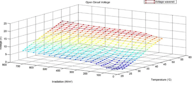
The different values of Vocfor all the possible range of irradiation and tem-perature in the target area is obtained like a net by pattern recognition to fit the value of collected data for 1 year. Figure 11 presents the wavenet of Voc, which can be easily used to retrieve Vocvalue for any couple of (G, T) data.

The solved experimental coefficients of Equation (14) are: a = 0.9943; α = 0.52727; βVoc= −0.02235.

This method allows also to get the a value, based on the measured and rec-orded values, and as such it fills the weakness of the Villalva’s method, which does not calculate a, but proposes to check it later.

5. Results and Discussion

The 1M3P and 1M4P are so easy to compute. All the algorithms of 1M5P models are implemented in MATLAB Software. In different environmental conditions than STC, all the methods presented (except our experimental method) are plot-ted with the equations for temperature adjustment in Section 4.1.2. Figure 11

demonstrated the high fitting of the Villalva’s and Modified Newton-Raphson methods from their I-V and P-V characteristics. NLS method presents I-V and P-V curves so near of the two others, but his Pmax is just less than Pmax,e. The form and the maximal value of these curves stem of the value of the ideality factor a, who is near to 1, but more than 1 (Table 2).

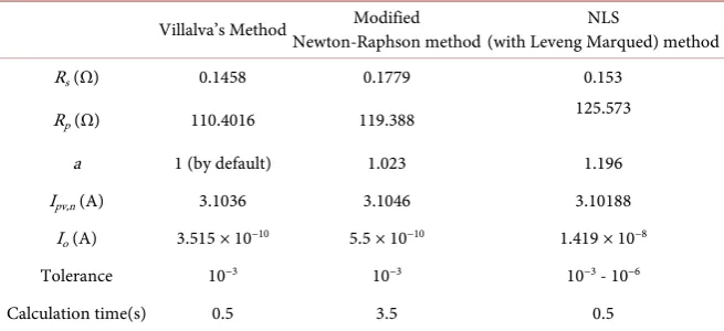
[image:15.595.211.537.563.708.2]

All the solution value of Rs presented in Table 2 are in the interval [0.13, 0.18], like showed on Figure 9. NLS and modified Newton Raphson lead to solve

(16)

[image:16.595.210.538.89.239.2]

Table 2. Parameters estimation of PV module LW-MS50.

Villalva’s Method _{Newton-Raphson method}Modified _{(with Leveng Marqued) method}NLS Rs (Ω) 0.1458 0.1779 0.153

Rp (Ω) 110.4016 119.388 125.573

a 1 (by default) 1.023 1.196 Ipv,n (A) 3.1036 3.1046 3.10188

Io (A) 3.515 × 10−10 5.5 × 10−10 1.419 × 10−8

Tolerance 10−3 ₁₀−3 ₁₀−3_{- 10}−6

Calculation time(s) 0.5 3.5 0.5

3 or 5 parameters directly. The optimization of multi-objective function using NLS through the Leveng Marqued method for solving the parameter estimation of a PV panel has been well done and the results are useful, comparable to classic iterative methods and less time-consuming. Nevertheless, the accuracy of esti-mated values depends upon the chosen tolerance band and initial conditions. However, in reason, of his calculation time, his simplicity and his reproducibili-ty, Rs and Rp from Villalva’s method is used in our proposed experimental me-thod and it’s called 1M5P in the following comments and Figure 12.

As a global result, Figure 13 shows three kinds of single-diode model in I-V and P-V curves, start from the model of 1M3P then this model adjusted with temperature (1M3P + T) and the model (1M5P) adjusted in temperature with (Rs, Rp) got by Villalva’s method from experimental data of the manufacturer. The measured power points are also presented.

Simulation of 1M4P, 1M3P model and of 1M3P+T is done with temperature coefficients extracted from the datasheet. These curves show a variation with the

Voc point following temperature variation. But the maximum simulated power is much higher than that measured. These models show their shortcomings in the face of reality.

On the other hand, the model 1M5P realized with the experimental data of the manufacturer but with the presence of Rs and Rp found through the iterative method, seems more realistic. The impact of Rp (smaller than in the model 1M4P, because neglected Rp comes to imagine a resistance in parallel very high like an open circuit) here considered creates a real fall of the maximum value of power and brings the Voc of this model near to the Voc measured under similar conditions of irradiation and temperature.

Regarding variations of Voc point through the models and their characteristics I-V, P-V, the value Voc(G, T) of our proposed experimental method very well matches the measured value when the output power is zero. The model is so ac-curate and overcomes the need claim by [36] to translate I-V and P-V for dif-ferent values of (G, T) than (G, T) at STC.

(17)

[image:17.595.61.539.73.276.2]

Figure 12. Comparison of three 1M5P models at STC.

Figure 13. P(V) and I(V) characteristics of different built models and data measurement G = 750 W/m2_;_T_{= 30˚C.}

calculated regression coefficient with a measured power output value is R2₌ 0.9869. Some points seem remote, they could be due to the wind speed (v) that was not stable (v < 1 m/s) and temperature changing, because the data are rec-orded every 1 minute. And the used temperatures for the simulation to obtain the characteristics I(V) and P(V) are the average during the variation period of the resistive load.

Figure 14 shows the mathematical P-V curve of 1M5P (get with reference’s points extracted from the datasheet), the proposed experimental method and measured curves in our tropical conditions of the LW-MS50 solar panel plotted at two different temperature and irradiation conditions. Figure 14 proves that 0 1 2 3 4 5 6 7 8 9 10 11 12 13 14 15 16 17 18 19 20 21 22 23 24 25

0 0.5 1 1.5 2 2.5 3 3.5 Voltage (V) C u rre n t (A ) NLS

Modified Newton Raphson Vivallva

0 1 2 3 4 5 6 7 8 9 10 11 12 13 14 15 16 17 18 19 20 21 22 23 24 25 0 10 20 30 40 50 60 Voltage (V) P ow er O ut put ( W ) NLS

Modified Newton Raphson Vivallva

1 2 3 4 5 6 7 8 9 10 11 12 13 14 15 16 17 18 19 20 21 22 23 24 25 0.5 1 1.5 2 2.5 3 3.5 Voltage (V) Int ens it y ( A )

current comparison of models

IntensityA vs. VoltageV experimental model I_G750 vs U_G750 (1M3P+T) I_T30C vs U_T30C(1M5P) I G750 vs U G750 (1M3P) I_G750 vs U_G750 (1M4P)

0 1 2 3 4 5 6 7 8 9 10 11 12 13 14 15 16 17 18 19 20 21 22 23 24 25 5 10 15 20 25 30 35

40 Power- Comparison models

Voltage (V) P o w e r (W )

[image:17.595.60.537.310.543.2]

(18)

[image:18.595.191.537.70.286.2]

Figure 14.P(V) curves comparison between proposed experimental model, 1M5P and mea-surement data.

1M5P (Vivallva’s model) strongly variates in irradiation and temperature as ex-pected: when irradiation increases, power increases, and for the temperature, the

Voc point decreases.

However, use this model although coming from experimentation (of the manufacturer) would cause many errors for the sizing of mini-plants in tropical area. Like, a lack of electrical energy when it’s not expected according to this model.

Comparison of power output from solar panel in real meteorological condi-tions and the model 1M5P with experimental datasheet points are done, with Equation (16).

measured model

measured

error P P

P

−

= _[13]₍₁₆₎

Table 3 represents the mean error and the standard deviation of these two groups of curves.

The relative error calculated is very high for large irradiation values. For both conditions, the error becomes increasing when the power decreases on the cha-racteristic curve. It is the moment of operation in the area “source of voltage” of the photovoltaic generator.

Also, when the solar radiation is around 600 W/m2_{and temperature: 30˚C, the} power is around 18 W, and this is at 12 AM to the worst month (August). But, the model with the manufacturer’s data reflects a power greater than 25 W (To 25˚C), thus, a decrease of 38.7%.

For this substitution, we can search for find other standards conditions for the geographical area, because the climatic data of the region over several years al-most never coincide with the NOCT or the STC.

0 2 4 6 8 10 12 14 16 18 20

5 10 15 20 25 30 35 40

Voltage (V)

P

ow

er (W

)

(19)

[image:19.595.211.537.93.152.2]

Table 3. Relative errors (%) between measured and 1M5P model power.

Panel powers _{relative error}Range of Average Standard deviation Peak power errors G = 750 W/m2_{; T = 35˚C [−8.2719; 0.9704] −1.8517} _1.8940 _−16.62%

G = 280 W/m2_{; T = 30˚C [−2.4673; 0.0463] −0.1712} _0.4022 _−12.50%

6. Conclusions

Following the high relationship between the input variables: irradiation, and temperature and the output power of the solar panel, the MPO of PV modules can be planned, if the solar irradiation and the ambient temperature are known. In the point of view of internal modeling, several models of electrical behavior have been developed for a common solar panel presents in a rural area. Our proposed 1M5P experimental model with the experimental coefficients obtained for different Voc(G, T) values turned out to be the one with the least errors in front of the values from the acquisition station deployed for the cause. This model was developed by previously the resistances (Rs, Rp), with iterative me-thods matching the manufacturer’s experimental MPO. However, this iterative method simply computes at different environmental conditions with tempera-ture coefficients of the manufactempera-turer gives errors, which alternate between 10% - 50% of the real power. Thus, the proposed experimental model leads to fit very well I-V and P-V curves from simulation to curves from measurement, and can be useful to obtain temperature coefficients on Voc and Isc more accurate in our environmental conditions than manufacturer’s proposition. Also, the choice to use the equation from two features I-V, P-V and their derivate by time, like in the NLS method, for obtaining these internal parameters contrary to a single characteristic higher used in the literature, improved the coincidence with the characteristics measured under different meteorological conditions.

In deduction, although through the search for a linear correlation between temperature and power, the coefficient of Pearson is less than 1 but not negligi-ble, this work validates the hypothesis that it is essential to consider temperature, in addition to irradiation, as an input vector to effectively estimate MPO. This raises the prospect of studying several solar cell temperature models as a func-tion of irradiafunc-tion, wind speed, ambient temperature and humidity, always in the same region. Also, our proposed method will be compared in future works with the Benchmark model to research the best experimental characterization and to simplify the optimization work of hybrid micro-central under tropical climate.

Conflicts of Interest

The authors declare no conflicts of interest regarding the publication of this paper.

References

(20)

Energy Agency, Paris.

[2] ERA (2006) Rapport préliminaire pour le Cameroun. ENEFBIO.

[3] Green, A. and Emery, K. (2008) Short Communication Solar Cell Efficiency Tables (Version 31). Progress in Photovoltaics, 16, 435-440.

https://doi.org/10.1002/pip.842

[4] Khan, M. and Iqbal, M. (2005) Dynamic Modeling and Simulation of a Small Wind-Fuel Cell Hybrid Energy System. Renewable Energy, 30, 421-439.

https://doi.org/10.1016/j.renene.2004.05.013

[5] Markvart, T. and Castaner, L. (2003) Practical Handbook of Photovoltaics, 2nd Edi-tion, Fundamentals and Applications, Elsevier, Amsterdam.

[6] King, D., Kratochvil, J., Boyson, W. and Bower, W. (1998) Field Experience with a New Performance Characterization Procedure for Photovoltaic Arrays. 2nd World Conference and Exhibition on Photovoltaic Solar Energy Conversion, Vienna, 6-10 July 1998.

[7] Kroposki, B., Marion, W., King, D., Boyson, W. and Kratochvil (2000) Comparison of Module Performance Characterization Methods. 28th IEEE PV Specialists Con-ference, Anchorage, 15-22 September 2000, 1407-1411.

https://doi.org/10.2172/772437

[8] Woyte, A., Nijs, J. and Belmans, R. (2003) Partial Shadowing of Photovoltaic Arrays with Different System Configurations. Literature Review and Field Test Results. So-lar Energy, 74, 217-233. https://doi.org/10.1016/S0038-092X(03)00155-5

[9] Gow, J.A. and Manning, C.D. (1999) Development of a Photovoltaic Array Model for Use in Power-Electronics Simulation Studies. IEE Proceedings—Electric Power Applications, 146, 193-200. https://doi.org/10.1049/ip-epa:19990116

[10] Xiao, W., Dunford, W. and Capel, A. (2004) A Novel Modeling Method for Photo-voltaic Cells. Power Electronics Specialists Conference, Aachen, 20-25 June 2004, 1950-1956.

[11] Walker, G. (2001) Evaluating MPPT Converter Topologies Using a Matlab PV Model. Journal of Electrical and Electronics Engineering, 21, 49-56.

[12] Sera, D., Teodorescu, R. and Rodriguez, P. (2007) PV Panel Model Based on Data-sheet Values. IEEE International Symposium, Vigo, 4-7 June 2007, 2392-2396.

https://doi.org/10.1109/ISIE.2007.4374981

[13] Koumi, S., Njomo, D. and Moungnutou, I. (2012) Comparison of Predictive Models for Photovoltaic Module Performance under Tropical Climate. Telkomnika, 10, 245-256. https://doi.org/10.12928/telkomnika.v10i2.783

[14] Lin, L. (2004) Investigation on Characteristics and Application of Hybrid So-lar/Wind Power Generation Systems. Hong Kong Polytechnic University, Hong Kong.

[15] Benmoussa, W.E.A. (2007) Etude comparative des modèles de la caractéristique courant-tension d’une cellule solaire au silicium monocristallin. Revue des Energies RenouvelablesICRESD-07, Tlemcen, 301-306.

[16] Ho’ang, A., Delinchant, B., et al. (2015) Renewable Energy Supply (PV) Integration with Building Energy Management: Modeling and Intelligent Control of Electrical Storage. Vietnam Academy of Science and Technology Journal of Science and Technology, 53, 173-187.

(21)

DOI: 10.4236/jpee.2019.75004 46 Journal of Power and Energy Engineering https://doi.org/10.1016/j.rser.2017.08.017

[18] Huang, Y., Lu, J., Liu, C., Xu, X., Wang, W. and Zhou, X. (2010) Comparative Study of Power Forecasting Methods for PV Stations. Proceedings of International Con-ference on Power System Technology (POWERCON), Hangzhou, 24-28 October 2010, 1-6. https://doi.org/10.1109/POWERCON.2010.5666688

[19] Pongratananukul, N. and Kasparis, T. (2004) Tool for Automated Simulation of So-lar Arrays Using General-Purpose Simulators. IEEE Workshop on Computers in Power Electronics, Urbana, 15-18 August 2004, 10-14.

[20] Hyvarinen, J. and Karila, J. (2003) New Analysis Method for Crystalline Silicon Cells. 3rd World Conference on Photovoltaic Energy Conversion, Osaka, 11-18 May 2003, 1521-1524. https://doi.org/10.1016/S1473-8325(03)00623-0

[21] Kensuke, N., Nobuhiro, S., Yukiharu, U. and Takashi, F. (2007) Analysis of Multi-crystalline Silicon Solar Cells by Modified 3-Diode Equivalent Circuit Model Taking Leakage Current through Periphery into Consideration. Solar Energy Material and Solar Cell, 91, 1222-1227. https://doi.org/10.1016/j.solmat.2007.04.009

[22] Carrero, C., Amador, J. and Arnaltes, S. (2007) A Single Procedure for Helping PV Designers to Select Silicon PV Module and Evaluate the Loss Resistances. Renewa-ble Energy, 32, 2579-2589. https://doi.org/10.1016/j.renene.2007.01.001

[23] Chin (2011) Fuzzy Logic Based MPPT for Photovoltaic Modules Influenced by Solar Irradiation and Cell Temperature. 13th International UkSim Conference on Model-ling and Simulation, Cambridge, 30 March-1 April 2011, 376-381.

https://doi.org/10.1109/UKSIM.2011.78

[24] Azzouzi, M., Popescu, D. and Bouchahdane, M. (2016) Modeling of Electrical Cha-racteristics of Photovoltaic Cell Considering Single-Diode Model. Journal of Clean Energy Technologies, 4, 414-420. https://doi.org/10.18178/JOCET.2016.4.6.323

[25] Rodrigues, E., Melício, R., Mendes, V. and Catalão, J. (2011) Simulation of a Solar Cell Considering Single-Diode Equivalent Circuit Model. Renewable Energies and Power Quality Journal, 1, 369-373. https://doi.org/10.24084/repqj09.339

[26] Hansen, A.D., Sorensen, P.E., Hansen, L.H. and Bindner, H.W. (2001) Models for a Stand-Alone PV System. Forskningscenter Risoe. Risoe-R, No. 1219.

[27] Hatziargyriou, N., Kariniotakis, G., Jenkins, N., Peças Lopes, J. and Oyarzabal, J. (2004) Modelling of ΜicroSources for Security Studies. CIGRE, Paris, 29 August-3 September 2004.

[28] Benavides, N.D. and Chapman, P.L. (2008) Modeling the Effect of Voltage Ripple on the Power Output of Photovoltaic Modules. IEEE Transactions on Industrial Electronics, 55, 2638-2643. https://doi.org/10.1109/TIE.2008.921442

[29] Benamara, V. (2012) Etude et simulation d’un panneau solaire raccordé au réseau avec périphérique de stockage.

[30] Hosseini, H., Farsadi, M., Lak, A., Ghahramani, H. and Razmjooy, N. (2012) A Novel Method Using Imperialist Competitive Algorithm (ICA) for Controlling Pitch Angle in Hybrid Wind and PV Array Energy Production System. Internation-al JournInternation-al on TechnicInternation-al and PhysicInternation-al Problems of Engineering, 4, 145-152.

[31] De Soto, W., Klein, S.A. and Beckman, W.A. (2006) Improvement and Validation of a Model for Photovoltaic Array Performance. Solar Energy, 80, 78-88.

https://doi.org/10.1016/j.solener.2005.06.010

[32] Ahmad, G.E., Hussein, H.M.S. and El-Ghetany, H.H. (2003) Theoretical Analysis and Experimental Verification of PV Modules. Renewable Energy, 28, 1159-1168.

(22)

[33] Vivallva, M. (2009) Modeling and Circuit-Based Simulation of Photovoltaic Arrays. 10th Brazilian Power Electronics Conference (COBEP), Bonito-Mato Grosso do Sul, 27 September-1 October 2009, 1244-1254.

https://doi.org/10.1109/COBEP.2009.5347680

[34] Hussein, A. (2017) A Simple Approach to Extract the Unknown Parameters of PV Modules. Turkish Journal of Electrical Engineering & Computer Sciences, 25, 4431-4444. https://doi.org/10.3906/elk-1703-14

[35] Tayyan, A. (2013) A Simple Method to Extract the Parameters of the Single-Diode Model of a PV System. Turkish Journal of Physics, 37, 121-131.

[36] Hadj Arab, A.C.F. and Benghanem, M. (2004) Loss-of-Load Probability of Photo-voltaic Water Pumping Systems. Solar Energy, 76, 713-723.