FORECASTING AND ANALYSIS MORTALITY USING LEE
*
Rana H. Shukur, Dr. Monem A. Mohammed and Shukr, H.
Agric. Engin. Ministry of Sci., Technol.
ARTICLE INFO ABSTRACT
We demonstrate here a model proposed by Lee and Carter (1992) for fit and to forecast mortality rates. This approach is used
Lee-Carter model allows for the construction of confidence intervals related to mortality and age death protections. To improve the performance of the Lee
version have been proposed. In this paper, we use real data of mortality rates by gender in Kirkuk City in Iraq during the period 2006
variations in age
Carter parameters model. We also use the autoregressive moving average (ARIMA) with the special case of Random walk with drift (RWD) model to forecast the
paper further predicts the survival expectancy at birth for each gender. Our results found this survival expectancy to be increasing for age group (0
the long
however on the available data.
Copyright © 2018, Rana H. Shukur et al. This is an open use, distribution, and reproduction in any medium, provided
INTRODUCTION
Studying and doing research on demography is a quantitative social science that deals with every aspect of human populations, such as marriage, divorce, giving birth, migration and finally death (Bell and Monsell, 1991). As human beings or population actors our final act on the earth is our death, and thus our death is one of the most important events in our life. It is a certainty that every one of us has been born and every one of us will die. In this research we will consider and analyse (Andreozzi, Blaconá Arnes 2011) the mortality of individual population actors (Carter and Prskawetz 2001) which is the most important event in our life. Lee and Carter (1992) presented a stochastic model, based on a factor analytic approach, to fit and predict mortality r Since then, because of its simplicity and relatively good performance, the Lee
demographic and actuarial applications in various countries. In addition, the Lee
by actuaries for multiple purposes. Essentially, the model assumes that the dynamic of mortality trends over time is only ruled by a single parameter called the mortality index. The mortality forecast is based on the index’s extrapolation, obtained by select appropriate time series model. The Box-Jenkins models, also known as an autoregressive moving average process (ARIMA) (Box and Jenkins, 1976), are usually used on forecasting. Lee and Carter (1996) used an random walk with drift (RWD) forecasting model. The RWD model does not make any assumption about the structure of the covariance matrix, while the Lee approach applies the estimation of the systematic non
on the Singular Value Decomposition (SVD) of an appropriate data matrix in this approach. Thus, the Lee more efficient when data are drawn with the Lee
mortality actors. Section (I) describes the properties of the Lee
Carter model is equivalent to a special type of multivariate random walk with drift (RWD) model, in which the covariance matr depends on the drift vector in section (II). In section (III) we use application data for Kirkuk City for the period 2006 Section (IV) we present some conclusions, and finally section (V) includes a brief discussion.
Measurements of Mortality
Mortality can be defined as “the frequency with which death occurs in the population”.
*Corresponding author: Rana H. Shukur,
Agric. Engin. Ministry of Sci., Technol.
ISSN: 0975-833X
Vol. 10, Issue, 10,
DOI: https://doi.org/10.24941/ijcr.
Article History:
Received 16th July, 2018 Received in revised form 27th August, 2018
Accepted 24th September, 2018 Published online 31st October, 2018
Citation:Rana H. Shukur, Dr. Monem A. Mohammed and Shukr, H. H.
application”, International Journal of Current Research
Key Words:
Death rates, Lee-Carter model, Singular Value Decomposition Time series Modeling; life Expectancy.
RESEARCH ARTICLE
FORECASTING AND ANALYSIS MORTALITY USING LEE-CARTER MODEL WITH APPLICATION
Rana H. Shukur, Dr. Monem A. Mohammed and Shukr, H.
Agric. Engin. Ministry of Sci., Technol.
ABSTRACT
We demonstrate here a model proposed by Lee and Carter (1992) for fit and to forecast mortality rates. This approach is used widely in demographical applications and academic literature because the structure of the
Carter model allows for the construction of confidence intervals related to mortality and age death protections. To improve the performance of the Lee-Carter model, several extensions to the original version have been proposed. In this paper, we use real data of mortality rates by gender in Kirkuk City in Iraq during the period 2006-2015 to apply a modification of the Lee
ariations in age-specific parameters using a singular values decomposition method to estimate the Lee Carter parameters model. We also use the autoregressive moving average (ARIMA) with the special case of Random walk with drift (RWD) model to forecast the general index for the time period 2015
paper further predicts the survival expectancy at birth for each gender. Our results found this survival expectancy to be increasing for age group (0-1) year and to be decreasing for age group (75
the long-term forecast it is necessary for the field of Demography to obtain such predications, which depend however on the available data.
open access article distributed under the Creative Commons Attribution provided the original work is properly cited.
demography is a quantitative social science that deals with every aspect of human populations, such as marriage, divorce, giving birth, migration and finally death (Bell and Monsell, 1991). As human beings or population our death, and thus our death is one of the most important events in our life. It is a certainty that every one of us has been born and every one of us will die. In this research we will consider and analyse (Andreozzi, Blaconá
ty of individual population actors (Carter and Prskawetz 2001) which is the most important event in our life. Lee and Carter (1992) presented a stochastic model, based on a factor analytic approach, to fit and predict mortality r
f its simplicity and relatively good performance, the Lee-Carter (LC) model has been widely used for demographic and actuarial applications in various countries. In addition, the Lee-Carter model and its extensions have been used purposes. Essentially, the model assumes that the dynamic of mortality trends over time is only ruled by a single parameter called the mortality index. The mortality forecast is based on the index’s extrapolation, obtained by select
Jenkins models, also known as an autoregressive moving average process (ARIMA) (Box and Jenkins, 1976), are usually used on forecasting. Lee and Carter (1996) used an random walk with drift (RWD) forecasting
not make any assumption about the structure of the covariance matrix, while the Lee approach applies the estimation of the systematic non-random structure Lee-Carter model to mortality forecasting, which is based
(SVD) of an appropriate data matrix in this approach. Thus, the Lee
more efficient when data are drawn with the Lee-Carter model. In this research we define a range of demographical concepts in e properties of the Lee-Carter model, and uses these properties to suggest that the Lee Carter model is equivalent to a special type of multivariate random walk with drift (RWD) model, in which the covariance matr
II). In section (III) we use application data for Kirkuk City for the period 2006 Section (IV) we present some conclusions, and finally section (V) includes a brief discussion.
with which death occurs in the population”.
International Journal of Current Research Vol. 10, Issue, 10, pp.74529-74537, October, 2018
DOI: https://doi.org/10.24941/ijcr.32671.10.2018
Rana H. Shukur, Dr. Monem A. Mohammed and Shukr, H. H. 2018. “Forecasting and Analysis Mortality using Lee
International Journal of Current Research, 10, (10), 74529-74537.
CARTER MODEL WITH APPLICATION
Rana H. Shukur, Dr. Monem A. Mohammed and Shukr, H. H.
We demonstrate here a model proposed by Lee and Carter (1992) for fit and to forecast mortality rates. This widely in demographical applications and academic literature because the structure of the Carter model allows for the construction of confidence intervals related to mortality and age-specific rter model, several extensions to the original version have been proposed. In this paper, we use real data of mortality rates by gender in Kirkuk City in 2015 to apply a modification of the Lee-Carter model, which accommodates specific parameters using a singular values decomposition method to estimate the Lee-Carter parameters model. We also use the autoregressive moving average (ARIMA) with the special case of
general index for the time period 2015-2020. The paper further predicts the survival expectancy at birth for each gender. Our results found this survival 1) year and to be decreasing for age group (75-80) years. For term forecast it is necessary for the field of Demography to obtain such predications, which depend
ribution License, which permits unrestricted
demography is a quantitative social science that deals with every aspect of human populations, such as marriage, divorce, giving birth, migration and finally death (Bell and Monsell, 1991). As human beings or population our death, and thus our death is one of the most important events in our life. It is a certainty that every one of us has been born and every one of us will die. In this research we will consider and analyse (Andreozzi, Blaconá and ty of individual population actors (Carter and Prskawetz 2001) which is the most important event in our life. Lee and Carter (1992) presented a stochastic model, based on a factor analytic approach, to fit and predict mortality rates. Carter (LC) model has been widely used for Carter model and its extensions have been used purposes. Essentially, the model assumes that the dynamic of mortality trends over time is only ruled by a single parameter called the mortality index. The mortality forecast is based on the index’s extrapolation, obtained by selecting an Jenkins models, also known as an autoregressive moving average process (ARIMA) (Box and Jenkins, 1976), are usually used on forecasting. Lee and Carter (1996) used an random walk with drift (RWD) forecasting not make any assumption about the structure of the covariance matrix, while the Lee-Carter Carter model to mortality forecasting, which is based (SVD) of an appropriate data matrix in this approach. Thus, the Lee-Carter estimator is Carter model. In this research we define a range of demographical concepts in Carter model, and uses these properties to suggest that the Lee-Carter model is equivalent to a special type of multivariate random walk with drift (RWD) model, in which the covariance matrix
II). In section (III) we use application data for Kirkuk City for the period 2006-2015. In
INTERNATIONAL JOURNAL OF CURRENT RESEARCH
The United Nations and the World Health Organization have proposed the following definition of death: “Death is the permanent disappearance of all evidence of life at any time after birth has taken place.” (I): Crude Death Rate (CDR): The simplest and most common measure of mortality is the crude death rate. The crude death rate is defined as:
CDR = ∗ 1000 (1-1)
Where (D) represents the total number of deaths in a given year, and (P) is the total mid-year population.
(II): Age-specific Death Rates (ASDR)
The risk of dying differs greatly with age, and this difference is not indicated by the crude death rate. That is why demographers often find it useful to use age-specific death rates. The age-specific death rate is defined as:
mx=
Dx
Px * 1000 (1-2)
Where (mx) is the age-specific death rate, (Dx) is the number of deaths of people aged (x) years since their last birthday, and (Px) is
the mid-year population of people aged (x) years.
(III): Life Expectancy at Birth: Age-specific life expectancy is an estimation of the average number of the remaining years that a person would be expected to live if current mortality conditions were constant.
Lee-Carter Method: The Lee and Carter model (named LC hereafter) is a demographic and statistical model that is used to project mortality rates (Lee and Carter, 1992). The method can be seen as a special case of a principal components method (Bozik and Bell, 1987; Bell and Monsell, 1991) with a single component. Therefore, this model’s extensions have been used by actuaries for multiple purposes. In addition, the LC model uses an autoregressive moving average process (ARIMA) with a special case of the random walk with drift (RWD) forecasting model.
Model description:
We can write the Lee–Carter model as follows:
m , = exp( , ) … (2-1)
Where the model’s basic premise is that there is a linear relationship among the age-specific death rates () and two explanatory factors: the initial age interval (x), and time (t). This means that the information is distributed in age intervals, so the interval that begins with the (x) age will be called "x age interval.
With(x = 0 − 1, 1 − 4, … , A) and (t = 1, 2, … , T)
Where:
, : Is the age-specific death rate for the (x)interval and the year (t) : Is the average age-specific mortality
: Is the mortality index in the year (t).
: Is a deviation in mortality due to changes in the ( ) index. , : Is the random error.
A:Is the beginning of the last age interval.
To solve (2-1) for estimate values of (ax, bx, and kt,), which are the solutions to the system, sowe can write the model in (2-1) as follows:
Log{ , } = { + + , } (2-2)
2-2: (Lee- Carter) model properties:
For properties (LC) model there is not a unique solution for this system. Consequently, it is necessary to add the following two constraints so as to obtain a unique solution:
1- ∑ = 1 ... (2-3)
2-∑ = 0 ... (2-4)
3-
→
, → (2-5)→ − , → + (2-6)
∀c ∈ R
Where (c) is constant.
Model Fitting: To a fitting model as in (2-2), we have a constraint which immediately implies that the parameter is simply the empirical average over time of the age profile in age group (x), then
^ =∑ ,
, withX = 1,2.3, … … . .Aand t=1,2,3… . .T
Where (A) is the last age of humans and (T) is the last year of data. Therefore ... (2-7)
Since practical uses of the Lee-Carter model implicitly assume that the disturbances ( are normally distributed, and then:{ , has a multiplicative fixed effects model for the centered age profile.Now let
(2-8)
… (2-9)
Where { } is the centered logged rates matrix as follows:Seen in this matrix, the Lee-Carter model can also be thought of as a
special case of a log-linear model for a contingency table. Indeed, this model is the most basic version of a contingency table model, where one assumes independence of rows (age groups) and columns (time periods), and the expected cell value is merely the product of the two parameter values from the respective marginal:
E(
In a contingency table model, this assumption would be appropriate if the variable represented as rows in the table was independent of the variable represented as columns. The same assumption for the log-mortality rate is the absence of (age× time interactions) that ( ) is fixed over time for all ( ) and ( ) is fixed over age groups for all (t).This system provides a unique solution when these constraints are included. All parameters on the right-hand side of equation (2-9) are unobservable, and fitting the model by the ordinary least squares method is impossible. To overcome this situation, we employ Lee and Carter’s (1992) two-stage estimation procedure, which gives exact solutions. In the first two-stage, singular value decomposition (SVD) is applied to the matrix of { } to obtain estimates of { }. This method is used to obtain the exact fitting of least squares (Good, 1969).Therefore, we get the following:
(2-10)
and (x) is a diagonal matrix.
(x): Singular Values matrix. (v): The Left Eigen Vectors Matrix
Therefore, we have:
(2-11)
... (2-12)
Therefore, we can write the above relationship as follows:
(2-13)
That means the first term of (2-13) represents the term, which depends on an estimate of all vectors of , but the second term represents the estimate of the standard error as follows:
(2-14)
Then, from (2-13) we can estimate all vectors as follows:
(2-15)
(2-16)
(2-17)
(2-18)
(2-19)
Where ( : The first column of the matrix (u).
( : The first column of the matrix (v).
: The first element of the diagonal matrix (x).
Second stage estimation: We can now use the re-estimate step to re-estimate the parameter ( ) by an iterative search using the
Newton Raph son method to get ( ). This re estimation step, often called “second stage estimation”, is to get a unique solution for the criterion and amore suitable estimation for mortality.
The Time series modeland forecasting: The second distinguishing feature of the Lee‐Carter approach is that, having reduced the time dimension of mortality to a single index( ), they use statistical time series methods to model and forecast this index. We
assume that time series ( ) follows an auto-regressive integrated moving average, ARIMA (p, d, q) as:
Where is the general time series,
: are unknown parametrics of the autoregressive model; : are unknown parametrics of the moving average model; and
{ } is a sequence of white noise random variables, iid with a mean (0) and constant Variance( ).To produce mortality forecasts, Lee and Carter, testing several ARIMA specifications, found that a random walk with drift (ARIMA(0,1,0))was the most appropriate model for mortality data; therefore, we can write ARIMA(0,1,0)
Where: (mortality index)as general time series in (t+s).
: ( is unknown, and denotes the drift parameter.
To estimate the drift parameter ( ), using (MLE) method as follows:
(2-21)
Which only depends on the first and last of the ( ) estimates. Moreover, we can write the variance error as follows:
(2-22)
The Forecasting of (ASDR): After estimates of all the parameters of the Lee–Carter model
(2-23)
(2-24)
, where (s) is the forecasting period with
Application Part: The following analysis describes the application of the Lee-Carter method(1992) to model, estimate, and forecast Age-specific Death Rates (ASDR)in Kirkuk. A general mortality index was created for each age and gender. The indexes were forecast using the ARIMA model and by using (Mat lab) software (Version 7). After forecasts were obtained, it was possible to project age-specific death rates and provide life expectancy at birth. Furthermore, projections of life expectancy at birth from official bodies were included so as to compare the results.
[image:5.595.137.466.498.776.2]Describe data and estimate model: Available data were composed of the population and death values both by age and gender in Kirkuk from 2006 to2015, and the data were provided by the Ministry of Health and the Ministry of planning. Thus, the age groups and gender mortality were estimated using the Lee-Carter method, and forecasting of the age-specific death rates was as follows:
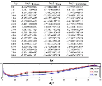
Table 3-1. The estimate parameter model ( ) for both female, male and total (2006-2015)
Age Female Male Combined 0.0 -4.69295810483 -4.78412821815 -4.49789453767 1.0 -6.78717989096 -6.47340256069 -6.81161166898 5.0 -8.14426194384 -7.56322010988 -7.79795991943 10.0 -8.40333158347 -7.53265604305 -7.86438139134 15.0 -7.87186036072 -6.81732489779 -7.19185845834 20.0 -7.65088904638 -6.16648131931 -6.61941882311 25.0 -7.44910360856 -5.91098588289 -6.37564576503 30.0 -7.36008388883 -5.88551954162 -6.35836146181 35.0 -7.08786071024 -5.83507739302 -6.27540667269 40.0 -6.76913845064 -5.71189137645 -6.09594791749 45.0 -6.43290254586 -5.53266641547 -5.88046273399 50.0 -5.62797531094 -5.11879795178 -5.33807513628 55.0 -5.12440023088 -4.51924377243 -4.78043380428 60.0 -4.58906734624 -4.10533654234 -4.32306577501 65.0 -4.10968427361 -3.57009218844 -3.80875059889 70.0 -3.37265189126 -3.12330711039 -3.2382097417 75.0 -2.87429880582 -2.65737640287 -2.76656074833 80.0 -3.3336884197 -3.46843935824 -3.40634205823
Now, we can find the estimate parameters as in (2-16) and (2-19) for both male, female and total (2006-2015) as in table (3-2).
To estimate the parameter ( ) by (SVD) method for both female, male and total (2006-2015)as in table (3-3).
[image:6.595.111.482.179.439.2]Now, to re-estimate the parameter ( ) by iterative search using the Newton Raphson method to get( ) as in table (3-4).
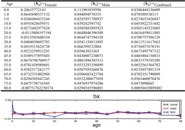
Table 3-2. Estimate parameter model ) for both female, male and total (2006-2015)
Age Female Male Combined
[image:6.595.132.464.502.612.2]0.0 0.20635772143 0.111901839596 0.0386444136609 1.0 0.0643690337132 0.044094578335 0.070580538315 5.0 0.0368484433244 0.0293951788937 0.0274653426847 10.0 0.0593828659551 0.039242593742 0.0453922331642 15.0 0.0273442977628 0.0505883895923 0.0565145523605 20.0 -0.0115808197194 0.0648046396509 0.0616459011085 25.0 0.0513503600334 0.0644747394338 0.0708757506129 30.0 0.0484050603783 0.0541154813495 0.0611511617663 35.0 0.0419515624738 0.066399532804 0.0756857678191 40.0 0.0523259913291 0.05863033365 0.0673495787332 45.0 0.0309157897603 0.0430007230073 0.0403804130833 50.0 0.0674796704917 0.0801894303513 0.0831579195289 55.0 0.0781438989681 0.0533291356099 0.0652561564782 60.0 0.0582517262177 0.0507959268876 0.0535057491319 65.0 0.0732531002984 0.0586683423704 0.0702351790099 70.0 0.0294305647245 0.0532208677058 0.0563460870476 75.0 0.0475738716385 0.0476937074206 0.0473090665 80.0 -0.00751762250374 0.0294545596001 0.00850418899482
Figure 3-2.Estimates parameter ) for female, male and total (2006-2015)
Table 3-3.The parameter model ( ) from (SVD) for both female, male and total (2006-2015)
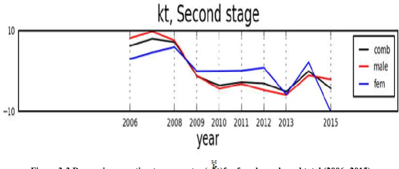
Table 3-4. Re-estimates the parameter ( ) for female, male and total (2006- 2015)
Year
( ) for Female ( ) for male ( ) for total 2006 3.76563271749 8.13027990038 6.24325485777 2007 4.65158525909 9.76428368969 7.98793956096 2008 6.08900207344 7.58023040235 7.17162301903 2009 0.20034052635 -1.0711107867 -1.17673255379 2010 -0.37059858611 -4.2401759385 -3.45113293463 2011 -0.48091197009 -3.0866339134 -2.62252725021 2012 -1.78761679328 -4.5730915541 -2.93459547062 2013 -6.2585628774 -5.7500560097 -4.94122976693 2014 0.02320713688 -0.9912842657 0.044127987258 2015 -3.94452798814 -1.9660901156 -4.15677197313 Year ( For female For male For total
[image:6.595.126.467.649.756.2]Figure 3-3.Decreasing re-estimate parameter ( )for female, male and total (2006- 2015)
[image:7.595.140.453.329.371.2]Forecasting mortality: To produce mortality forecasts, Lee and Carter(1992) assumed that the most appropriate model wasa random walk with drift (RWD) or (ARIMA)(0, 1,0) model as in (2-20).Thus, according to our mortality data,we found forecasting values( ) and (
)
as in (3-5) and (3-6) tables.Table 3-5. Forecasting values ( ) with standard error (See) for female, male and total
Item See Sec
[image:7.595.101.502.414.477.2]Female -0.85668 Male -1.12181 Total -1.15555
Table 3-6. Forecasting values ( ) for female, male and total
years -female S.E. -male S.E. -total S.E. 2016 -0.8566 3.6542 -1.121819 3.677158 -1.155559 3.749441 2017 -1.7133 5.4200 -2.243638 5.454106 -2.311117 5.561320 2018 -2.5700 6.9333 -3.365457 6.976916 -3.466676 7.114064 2019 -3.4267 8.3328 -4.487276 8.385209 -4.622234 8.550041 2020 -4.2834 9.6681 -5.609094 9.728845 -5.777793 9.920089
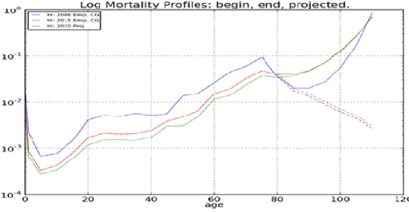
Now, substituting ( ) and in (Lee-Carter) as in (2-2) model to forecast the values of log-mortality as in the following figures:
Figure 3-5. Forecast the values of log-mortality for Male with actual data (2006- 2015) and forecasting values in (2020).
Figure 3-6.Forecast the values of log-mortality for Total with actual data (2006- 2015) and forecasting values in (2020).
DISCUSSION AND CONCLUSION
In this paper the application of the Lee-Carter model to specific ages has been described in relation to mortality rates by gender in Kirkuk, Iraq. The conclusions of this research are as follows:
The estimates of the average age-specific mortality parameter ( are available for the period 2006-2015, which is increasing for the age group (0-1) year and decreasing for the age group (75-80) years.
We have shown from an analysis of average age-specific mortality and an estimate of (
)
and ) parameters, that using the (SVD) method plays an important rule for identifying trends in mortality for the period of estimation and forecasting. We computed (18) age groups for each gender index; levels for mortality and coefficients were obtained through the
Lee-Carter method.
The general index of mortality and forecasting for the period 2016-2020 used the important method (Box-Jenkins) such
that (ARIMA) (0,1,0) model.
Forecast models such as ARIMA(0, 1, 0), with a constant, was used to project the ( ) index and presented an adequate
fit model.
According to the forecast method used, such rates showed increasing and decreasing mortality depending on different times and ages.
The long-term forecast was necessary for the field of Demography and obtaining them depends on the available data.
REFERENCES
Andreozzi, L., Blaconá, M.T and Arnes, N. 2011. The Lee-Carter Method for Estimating and Forecasting Mortality: An Application for Argentina, School of Statistics Faculty of Economics and Statistics, National University of Rosario, Argentina. Bell. W.R. and Monsell. B. 1991. Using principal components in time series modeling and forecasting of age-specific mortality
rates. Proceedings of the American Statistical Association -Social Statistics Section: 154-159.
Box, G. and Jenkins, G. M. 1976. Time Series Analysis Forecasting and Control. 2nd ed. San Francisco: Holden-Day.
Carter, L. R. and Prskawetz, A. 2001. Examining Structural Shifts in Mortality Using the Lee-Carter Method, Max Planck Institute for Demographic Research WP 2001-007, Germany.
Lee, R. D., 1993. Modeling and forecasting the time series of U.S. fertility age distribution range, and ultimate level, International
Journal of Forecasting, 9: 187-202.
Lee. R. D. and Carter. L. 1992. Modeling and Forecasting the Time Series of U.S. Mortality, Journal of the American Statistical
Association, 87:659-71.
Wang. J.Z.2007. Fitting and Forecasting Mortality for Sweden: Applying for the Lee-Carter Model, Mathematical Statistics, Stockholm University.
Wei, W.S. 1989. Time series analysis: Univariate and multivariate methods, New York, NY: Addison Wesley.
Wilmoth. J. R. 1993. Computational Methods for Fitting and Extrapolating the Lee-Carter Model of Mortality change. Technical Report - Department of demography, University of California, Berkeley.