Abstract—In this work, a novel gate-level delay computing method for common subexpression elimination (CSE) algorithm is proposed. The computing method is based on delay matrix and suitable for implementationwith computers. A CSE algorithm with gate-level delay computing (GLDC-CSE) is developed. The GLDC-CSE algorithm is demonstrated through a case study in AES S-box implementation with composite field arithmetic (CFA). Experimental results have shown that the period of delay computing accounts for 34.46% of GLDC-CSE algorithm running time on an average. Using GLDC-CSE algorithm, the gate counts and area-delay-production (ADP) of constant matrix multiplications in AES S-box is reduced by 39.20% and 28.56% respectively on an average. Also, the minimal area combination of matrices and the shortest critical path delay (CPD) combination of matrices can be determined by using GLDC-CSE algorithm, respectively.
Index Terms—gate-level delay computing, common subexpression elimination, critical path delay, multiple constant multiplication, composite field arithmetic.
I. INTRODUCTION
ULTIPLE constant multiplication (MCM) is widely used in many digital signal processing (DSP) applications, such as digital filtering, image processing, linear transforms, etc. In high level synthesis of VLSI design, the optimization of MCMs can lead to significant improvements in various design parameters like area or power consumption. Common subexpression elimination (CSE) is an effective optimization method to solve the MCM problems . The idea of CSE is to identify patterns (common subexpressions) that are present in expressions more than once and replace them with a single variable. With this, each of these patterns needs only to be computed once, thus reducing the size of the hardware required in VLSI implementation. However, how to select a
Manuscript received June 17, 2013; revised August 20, 2013. This work was supported by the National Natural Science Foundation of China (61376025 and 61106018), Industry-academic Joint Technological Innovations Fund Project of Jiangsu (BY2013003-11).
Ning Wu is with the College of Electrical and Information Engineering, Nanjing University of Aeronautics and Astronautics (NUAA), Nanjing 210016, China (e-mail: [email protected]).
Xiaoqiang Zhang is with the College of Electrical and Information Engineering, NUAA, Nanjing 210016, China (e-mail: [email protected]). Yunfei Ye is with the College of Electrical and Information Engineering, NUAA, Nanjing 210016, China (e-mail: [email protected]).
Lidong Lan is with the College of Electrical and Information Engineering,
pattern to eliminate for achieving optimal results is an NP-complete problem [1]–[2].
Constant matrix multiplications over Galois field is a special case of the MCM problem, which is widely used in cryptography and coding theory, because in the Galois field, addition is performed via XOR and multiplication is performed in several different ways. Many CSE algorithms have been used to reduce the complexity architectures for constant matrix multiplications over Galois field [1]–[10].
Both area and throughput are significant for VLSI design. Previous CSE algorithms mostly focused on reducing the area complexity without providing complete control on the CPD, which ultimately determines throughput [11]. The delay is easy to determine for a straightforward implementation of constant matrix multiplication. CSE algorithms try to reduce the area complexity via transforming the constant matrix. Thus, the first challenge for the CPD control of a CSE algorithm is how to compute the delay associated with each transformation of the matrix. Chen et al. first proposed a gate-level delay computing method for CSE algorithm based on restriction graph [11]. The method selects a restriction graph to represent the transformed constant matrix after running a CSE algorithm, and the CPD can be determined by translating the restriction graph to an optimal XOR tree. Both restriction graph transforming and optimal XOR tree translating are needed to complete the complicated operations.
In this paper, a new gate-level delay computing method for CSE algorithm is proposed. The new method is based on a delay matrix and should be carried out with CSE algorithm simultaneously. Since our method adopts matrix form in the computing process, compared with the method presented in [11], which adopts restriction graph form, our method is more suitable for implementation with computers.
The rest of the paper is organized as follows. Section II describes the basic principles of CSE algorithm. The detailed description of the new gate-level delay computing method is introduced in section III. In section IV, a CSE algorithm with gate-level delay computing (GLDC-CSE) is proposed and demonstrated through a case study in implementation of AES S-box based on composite field arithmetic (CFA). Finally, the conclusions are given in Section V.
II. THE BASIC PRINCIPLES OF CSEALGORITHM
MCM over Galois field can be expressed as a linear transform Y = MX, where Y and X are m- and n-dimensional column vectors, respectively, and M is an m×n constant
Improving Common Subexpression Elimination
Algorithm with A New Gate-Level Delay
Computing Method
Ning Wu, Xiaoqiang Zhang, Yunfei Ye, and Lidong Lan
matrix over the Galois field [1]–[2]. X represents the input variables and Y represents the output variables, while M indicates the set of constant coefficients. Clearly, such a transform requires only additions. Take note that, additions over Galois Field are referring to XOR operation, and hence the MCM over Galois Field can be implemented by a combinational logic with XOR gates only.
The linear transform Y = MX can be expressed in bit-level equations. A CSE algorithm can be exploited to extract the common factors in all the bit-level equations, in order to reduce the area cost of combinational logic implementation. In general, any CSE algorithm involves the following general steps [2]:
1) Identify patterns (common factors) that are present in the transformation.
2) Select a pattern for elimination.
3) Remove all the occurrences of the selected pattern. 4) The eliminated pattern is computed only once.
5) Repeat Step 1-4 until none of multiple patterns is present.
Consider the computation as follows:
0 0 0 1 2 3 4
1 1 0 1 3 4
2 2 0 1
3 3 0 1 3
4 4 2
1 1 1 1 1 1 1 0 1 1 1 1 0 0 0 1 1 0 1 0 0 0 1 0 0
y x x x x x x
y x x x x x
y x x x
y x x x x
y x x
(1)
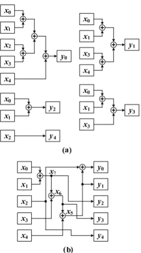
[image:2.595.331.530.54.466.2]A simple CSE algorithm applied to (1) is illustrated in Fig.1. The CSE algorithm identifies “x0+x1+x3+x4” as the
pattern in the first iterative, and generates a new variable “x5”
to replace it. The identified pattern is appended to the bottom of constant matrix as an additional row to be further optimized by the CSE algorithm. In the following iterative, the patterns “x0+x1+x3” and “x0+x1” are identified and
replaced by variables “x6” and “x7” respectively.
A straightforward realization of computation in (1) is shown in Fig.2(a) which requires 10 XOR gates. However, after the CSE optimization, there are only 4 XOR gates required to realize, as illustrated in Fig.2(b). The reduction of XOR gates can be up to 60%.
III. GATE-LEVEL DELAY COMPUTING METHOD BASED ON
DELAY MATRIX
In this section, a new gate-level delay computing method for CSE algorithm is proposed. A similar method has been presented in [11], which is based on a restriction graph. The restriction-graph-based method should be carried out after running a CSE algorithm, and the computing process of the method can be divided into three steps:
1) Establish a restriction graph based on the transformed constant matrix after running a CSE algorithm.
2) Translate the restriction graph to an optimal XOR tree. 3) Compute delay value based on the optimal XOR tree and
determine the CPD.
Same as the method in [11], the method presented in this
paper can be also divided into three steps: Fig. 2 Realization of the computation in (1). (a) Straightforward realization. (b) After optimized by the simple CSE algorithm. 1 1 1 1 1
1 1 0 1 1 1 1 0 0 0 1 1 0 1 0 0 0 1 0 0
0 0 1 2 3 4
1 0 1 3 4
2 0 1
3 0 1 3 4 2
y x x x x x
y x x x x
y x x
y x x x
y x
Matrix Equations
0 0 1 0 0 1 0 0 0 0 0 1 1 1 0 0 0 0 1 1 0 1 0 0 0 0 1 0 0 0 1 1 0 1 1 0
Pattern1Elimination
0 2 5
1 5 2 0 1
3 0 1 3
4 2
5 0 1 3 4
y x x
y x
y x x
y x x x
y x
x x x x x
0 0 1 0 0 1 0 0 0 0 0 0 1 0 1 1 0 0 0 0 0 0 0 0 0 0 0 1 0 0 1 0 0 0 0 0 0 0 0 1 0 1 1 1 0 1 0 0 0
0 2 5
1 5
2 0 1
3 6 4 2
5 4 6
6 0 1 3
y x x
y x
y x x
y x
y x
x x x
x x x x
Pattern2Elimination
0 0 1 0 0 1 0 0 0 0 0 0 0 1 0 0 0 0 0 0 0 0 0 1 0 0 0 0 0 0 1 0 0 0 1 0 0 0 0 0 0 0 0 0 1 0 1 0 0 0 0 1 0 0 0 1 1 1 0 0 0 0 0 0
Pattern3Elimination
0 2 5
1 5 2 7
3 6 4 2 5 4 6
6 3 7 7 0 1
y x x
y x
y x
y x
y x
x x x
x x x
x x x
[image:2.595.49.288.322.397.2]
[image:2.595.358.500.489.742.2]1) Establish a initial delay matrix based on the primitive constant matrix before running a CSE algorithm. 2) Update delay matrix during a CSE algorithm running. 3) Compute delay value based on the delay matrix and
determine the CPD.
Different from [11], our method is based on a delay matrix and should be carried out with CSE algorithm simultaneously. The details of our delay computing method will be described below.
A. Establish Initial Delay Matrix
Consider a constant matrix M, in which a row corresponds to an output variable and a column corresponds to an input variable. In a row of constant matrix M, “1” represents that the input variable participates in computing of the output variable, and therefore the initial delay value of the input variable should be set to 0. On the other hand, “0” represents that the input variable does not participate in computing of the output variable, and therefore the initial delay value of the input variable should be invalid. Digit “–1” can be chose to represent the invalid value. According to the above discussion, an initial delay matrix Md can be obtained by formula:
1 d
M M M (2)
where M is the constant matrix and M1 is a matrix that has the
same dimension as M, and all elements value of M1 is 1.
According to (3), the initial delay matrix Md1 of (1) can be
figured out as follows:
1
1 1 1 1 1 1 1 1 1 1 1 1 0 1 1 1 1 1 1 1 1 1 0 0 0 1 1 1 1 1 1 1 0 1 0 1 1 1 1 1 0 0 1 0 0 1 1 1 1 1
0 0 0 0 0
0 0 1 0 0
0 0 1 1 0
0 0 1 1 1
1 1 0 1 1
d
M
(3)
B. Update Delay Matrix
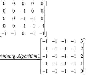
The constant matrix M has been changed during the running period of a CSE algorithm, therefore the delay matrix should be updated accordingly. During a CSE algorithm running, suppose that a pattern “xi+xj+…+xk” is replaced by a new variable “xnew” and appended to the bottom of constant matrix as an additional row. Suppose the delay value of “xnew” is represented by “dnew” and the delay value of “xi”, “xj” , ... , and “xk” is represented by “di”, “dj” , ... , and “dk” respectively. Correspondingly, an additional row should be appended to the bottom of delay matrix according to the “di”, “dj” , ... , and “dk”. Then “dnew” can be figured out by running Algorithm 1 according to the additional row of delay matrix.
Algorithm 1: Compute Delay Value
1) Input a row of delay value d0 d1 …dn (n≥2).
2) Sort the row in an increasing order.
3) Select the smallest two delay values di and di+1 which
is no less than 0.
4) Update new values of di and di+1 using the following
equations:
1 max( , 1) 1;
1;
i i i
i
d d d d
(4)
5) Repeat steps 2-4 until there is only the last delay value dn no less than 0.
Note that Algorithm 1 is essentially as same as Algorithm 2 in [11] and algorithm in Fig.4 in [12], both of which are used to compute delay value of output variable from an optimal XOR tree, and the latter has been proved to be optimal in [12]. After running Algorithm 1, “dnew” is the computing result of “dn” in Algorithm 1. The updated process of “dnew” is described below.
Algorithm 2: Update Delay Value
1) Append new row with “di”, “dj”, ... , and “dk” according to the transformation of constant matrix M. 2) Append new column with “dnew” according to the
transformation of constant matrix M.
3) Detect the row-number of the position of “dnew”, if the row-number “l” is greater than the maximum-row-number “m-1” of original matrix (suppose the original matrix is m×n-dimensional matrix), re-compute and re-update the delay value “dl”.
4) Take delay value “dl” as “dnew” to repeat step 3, until there is no row-number of the position of “dnew” that is greater than the maximum-row- number “m-1”. Consider the computation in (1), a new variable “x5”
replaces the pattern “x0+x1+x3+x4” in the first iterative of the
CSE algorithm. The updated process of constant matrix M is shown in Fig.1. The corresponding updated process of delay matrix can be expressed as follows:
0 0 0 0 0
0 0 1 0 0
0 0 1 1 0
0 0 1 1 1
1 1 0 1 1
0 0 0 0 0
0 0 1 0 0
0 0 1 1 0
0 0 1 1 1
1 1 0 1 1
0 0 1 0 0
append new row
5
1 1 0 1 1 2
1 1 1 1 1 2
0 0 1 1 1 1
0 0 1 0 1 1
1 1 0 1 1 1
0 0 1 0 0 1
compute d and append new column
(5)
In the second iterative, the pattern “x0+x1+x3” is replaced
by “x6”. The updated process of delay matrix can be
expressed as follows:
1 1 0 1 1 2
1 1 1 1 1 2
0 0 1 1 1 1
0 0 1 0 1 1
1 1 0 1 1 1
0 0 1 0 0 1
1 1 0 1 1 2
1 1 1 1 1 2
0 0 1 1 1 1
0 0 1 0 1 1
1 1 0 1 1 1
0 0 1 0 0 1
0 0 1 0 1 1
append new row
6
1 1 0 1 1 2 1
1 1 1 1 1 2 1
0 0 1 1 1 1 1
1 1 1 1 1 1 2
1 1 0 1 1 1 1
1 1 1 1 0 1 2
0 0 1 0 1 1 1
compute d and append new column
5
1 1 0 1 1 3 1
1 1 1 1 1 3 1
0 0 1 1 1 1 1
1 1 1 1 1 1 2
1 1 0 1 1 1 1
1 1 1 1 0 1 2
0 0 1 0 1 1 1
recompute d (6)
The original constant matrix M of computation in (1) is 5×5-dimensional matrix. As shown in (6), the row-numbers of the positions of “d6” are 3 and 5, respectively. Among
which, 5 is greater than 4, which is the maximum-row- number of original constant matrix M. Therefore “d5” shall be
re-computed and re-updated again.
Likewise, the updated process of delay matrix in the last iterative can be expressed as follows:
1 1 0 1 1 3 1
1 1 1 1 1 3 1
0 0 1 1 1 1 1
1 1 1 1 1 1 2
1 1 0 1 1 1 1
1 1 1 1 0 1 2
0 0 1 0 1 1 1
1 1 0 1 1 3 1
1 1 1 1 1 3 1
0 0 1 1 1 1 1
1 1 1 1 1 1 2
1 1 0 1 1 1 1
1 1 1 1 0 1 2
0 0 1 0 1 1 1
0 0 1 1 1 1 1
append new row
7
1 1 0 1 1 3 1 1
1 1 1 1 1 3 1 1
1 1 1 1 1 1 1 1
1 1 1 1 1 1 2 1
1 1 0 1 1 1 1 1
1 1 1 1 0 1 2 1
1 1 1 0 1 1 1 1
0 0 1 1 1 1 1 1
compute d and append new column
6 5
1 1 0 1 1 3 1 1
1 1 1 1 1 3 1 1
1 1 1 1 1 1 1 1
1 1 1 1 1 1 2 1
1 1 0 1 1 1 1 1
1 1 1 1 0 1 2 1
1 1 1 0 1 1 1 1
0 0 1 1 1 1 1 1
recompute d and d
(7)
C. Determine the CPD
After running the CSE algorithm, the delay value of each output variable can be determined by running Algorithm 1 for first m rows of delay matrix. Considering the computation in (1), the computing result of each output variable delay value is shown as follows:
1 1 0 1 1 3 1 1
1 1 1 1 1 3 1 1
1 1 1 1 1 1 1 1
1 1 1 1 1 1 2 1
1 1 0 1 1 1 1 1
1 1 1 1 1 1 1 4
1 1 1 1 1 1 1 3
1 1 1 1 1 1 1 1 1
1 1 1 1 1 1 1 2
1 1 1 1 1 1 1 0
The maximum delay value of computing results in (8) is 4, hence the CPD value of circuit structure optimized with the CSE algorithm, as shown in Fig.2(b), is 4 XOR gates. From Fig.2(b), the path from x0 to y0 and the path from x1 to y0 can
be determined as critical path.
The CPD value of circuit structure in Fig.2(a) can be determined from initial delay matrix in (3) via running Algorithm 1, and the computing result is shown as follows:
0 0 0 0 0
0 0 1 0 0
0 0 1 1 0
0 0 1 1 1
1 1 0 1 1
1 1 1 1 3
1 1 1 1 2
1 1 1 1 1 2
1 1 1 1 1
1 1 1 1 0
running Algorithm
(9)
According to (9), the CPD value of circuit structure in Fig.2(a) is 3 XOR gates, which is shorter than the one in Fig.2(b). This is because the circuit structure of MCM before any CSE transformations has the shortest CPD [11].
IV. GLDC-CSE AND ITS APPLICATION
In this section, we will illustrate our gate-level delay computing method by applying it to an existing CSE algorithm proposed in [4]. This algorithm is based on an iterative pairwise matching heuristic. More details of this CSE algorithm can be found in [4]. A new CSE algorithm named GLDC-CSE is developed that combines the CSE algorithm with the delay computing method proposed in this paper.
In the following, the GLDC-CSE algorithm is demonstrated by applying it to binary linear transformations for Advanced Encryption Standard (AES) S-box implementation with CFA. AES is a symmetric block encryption standard selected by NIST to replace the Data Encryption Standard (DES) in 2001. AES algorithm performs four transformations, namely SubBytes, ShiftRows, MixColumns and AddRoundKey through out the encryption process. The SubBytes, commonly known as S-box, consists of a multiplicative inverse over GF(28) followed by an affine
transformation. The S-box can be described as:
1
YMX C (10)
where M is an 8×8 binary constant matrix of affine transformation, C is an 8-bit binary constant vector of affine transformation, and X and Y represent 8-bit input vector and output vector respectively. CFA has been widely utilized in designing an optimized combinatorial circuit of AES S-box [2], [6]–[7], [11], [13]. CFA can be built iteratively from the lower order fields in order to simplify mathematical manipulation. By using CFA, the multiplicative inverse over GF(28) can be mapped to the subfield (either GF(24) or
GF(22)), hence an isomorphism function and its inverse are
required for mapping. The S-box with CFA can be described as:
1 1
( ( ) )
YM X C (11)
where β is an 8×8 binary matrix of isomorphism function and β–1 is an 8×8 binary matrix of inverse isomorphism function.
The inverse isomorphism matrix β–1 and affine
transformation matrix M are both linear transformations, so they can be merged into a new matrix L = Mβ–1 to reduce the
gate count. The new matrix L is named “Inverse Isomorphism-Affine Transformation (II-AT) matrix” in the following. Both isomorphism matrix and II-AT matrix are 8×8 binary matrices. Then, CSE algorithm could be performed to reduce the common factors in the equations effectively.
Composite field can be constructed by using different isomorphism matrices. There are 432 isomorphism matrices for mapping 8-bit vector from GF(28) to the subfield [6]. An
algorithm for isomorphism matrices generation can be found in [13]. In the following, Eight isomorphism matrices (β0~β7) ), which are generated by the algorithm in [13] in the
case of {ф=(10)2, λ=(1100)2}, and their corresponding II-AT
matrices (L0~L7) are taken to test the performance of
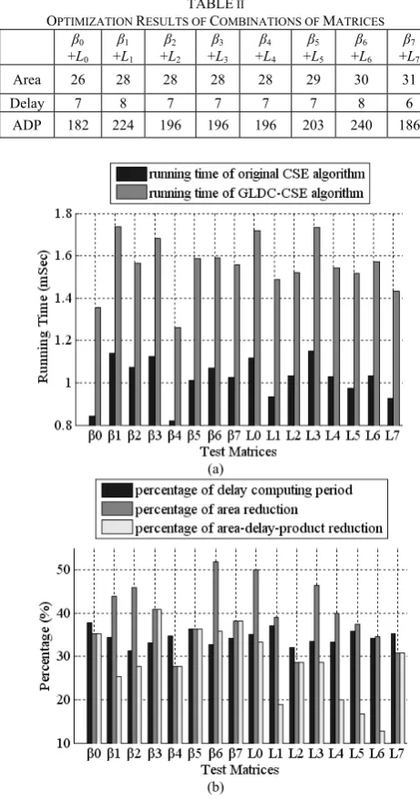
GLDC-CSE algorithm. Fig.3(a) shows the running time of each matrix optimized by original CSE algorithm in [4] and GLDC-CSE algorithm proposed in this paper. The value in Fig.3(a) is an average of the periods of 10 times runing repeatedly with Matlab. The GLDC-CSE algorithm combine the CSE algorithm in [4] with the delay computing method proposed in this paper, so the period of delay computing is the difference of running time between original CSE algorithm and GLDC-CSE algorithm. The periods of delay computing account for the periods of GLDC-CSE algorithm running time is shown in Fig.3(b). Fig.3(b) also shows area reduction percentage and ADP reduction percentage of each matrix optimized by GLDC-CSE. The performance of GLDC-CSE algorithm can be summarized in table I.
In the determination of the optimal composite field construction, both isomorphism matrices and II-AT matrices should be considered together. Table II shows the sum of optimization results of isomorphism matrices and II-AT matrices optimized by GLDC-CSE algorithm. As shown in table II, combination of matrices β0+L0 has the minimal total
area and ADP. Although combination of matrices β7+L7 has
the largest total area, it has the shortest CPD.
TABLEI
SUMMARIES OF GLDC-CSEALGORITHM PERFORMANCE
Performance minimal maximum average GLDC-CSE Running Time (mS) 1.2605 1.7358 1.5536
[image:5.595.49.258.161.311.2]V. CONCLUSION
In this work, a novel gate-level delay computing method based on delay matrix is proposed. The proposed computing method adopts matrix form, so it is more simple and more easy to be implemented than restriction graph form presented in [11]. Combining our gate-level delay computing with an existing CSE algorithm, a GLDC-CSE algorithm is developed. A case study in AES S-box implementation with CFA shows that the period of delay computing accounts for 34.46% of GLDC-CSE algorithm running time on average, and the gate counts and area-delay-production (ADP) of constant matrix multiplications in AES S-box is reduced by 39.20% and 28.56% respectively on average by using GLDC-CSE algorithm. The GLDC-CSE algorithm also can determine the minimal area combination of matrices and the shortest critical path delay (CPD) combination of matrices respectively.
REFERENCES
[1] N. Chen, and Z. Y. Yan, “Cyclotomic FFTs With Reduced Additive Complexities Based on a Novel Common Subexpression Elimination Algorithm,” IEEE Trans. Signal Processing, Vol. 57, no. 3, pp. 1010-1020, Mar. 2009.
[2] M. M. Wong, and M. L. D. Wong, “A new common subexpression elimination algorithm with application in composite field AES S-box,” Tenth Int. Conf. Information Sciences Signal Processing and their
Applications (ISSPA 2010), pp. 452-455, May 2010.
[3] C. Paar, “Optimized arithmetic for Reed-Solomon encoders,” in Proc.
IEEE International Symp. Inf. Theory, p. 250, June-July 1997.
[4] Y. Chen, and K. K. Parhi,, “Small Area Parallel Chien Search Architectures for Long BCH Codes,” IEEE Transaction on Very Large
Scale Integration (VLSI) systems, Vol. 12, No. 5, pp.545-549, May
2004.
[5] Q. Hu, Z. Wang, J. Zhang and J. Xiao, “Low Complexity Parallel Chien Search Architecture for RS Decoder,” IEEE International Symposium
on Circuits and Systems, 2005 (ISCAS 2005), Vol. 1, pp.340-343.
[6] D. Canright, “A very compact Rijndael S-box,” Technical report
NPSMA-04-001, Naval Postgraduate School, 2005.
[7] S. Hsiao, M. Chen, and C. Tu, “Memory-free low-cost designs of Advanced Encryption Standard using common subexpression elimination for subfunctions in transformations,” IEEE Trans. Circuits Syst. I, vol. 53, no. 3, pp. 615-626, 2006.
[8] O. Gustafsson and M. Olofsson, “Complexity Reduction of Constant Matrix Computations over the Binary Field,” First International
Workshop on Arithmetic of Finite Fields (WAIFI 2007),
Springer-Verlag, LNCS 4547, pp. 103–115, 2007.
[9] Y. Lee, H. Yoo, and I.-C. Park, “ Low-Complexity Parallel Chien Search Structure Using Two-Dimensional Optimization,” IEEE
Transaction on Circuits and Systems—II: Express Briefs, Vol. 58, No.
8, pp.522-526, August 2011.
[10] S. Bellini, M. Ferrari, and A. Tomasoni, “On the Structure of Cyclotomic Fourier Transforms and Their Applications to Reed-Solomon Codes,” IEEE Transactions on Communications, Vol. 59, No. 8, pp.2110-2118, August 2011.
[11] N. Chen, and Z. Y. Yan, “High-Performance Designs of AES Transformations,” IEEE International Symposium on Circuits and
Systems (ISCAS 2009), 2009, pp. 2906 – 2909.
[12] N. Petra, D. De Caro, and A. G. M. Strollo, “A novel architecture for Galois fields GF(2m) multipliers based on Mastrovito scheme,” IEEE
Trans. Comput., vol. 56, no. 11, pp. 1470–1483, Nov. 2007.
[13] X. Zhang and K. K. Parhi, “On the optimum constructions of composite field for the AES algorithm,” IEEE Transaction on Circuits and
systems–II: Express Briefs, vol. 53, no. 10, pp. 1153–1157, Oct. 2006.
(a)
(b)
Fig. 3 Perfomance of GLDC-CSE Algorithm. (a) Running time of Paar’s algorithm and GLDC-CSE algorithm. (b) Percentage of delay
computing period, area reduction and ADP reduction. TABLE II
OPTIMIZATION RESULTS OF COMBINATIONS OF MATRICES β0
+L0 β1 +L1
β2 +L2
β3 +L3
β4 +L4
β5 +L5
β6 +L6
β7 +L7 Area 26 28 28 28 28 29 30 31
Delay 7 8 7 7 7 7 8 6
[image:6.595.50.281.57.497.2]