Using Clarke and Wright’s Algorithm to Minimize
the Machining Time of Free-Form Surfaces in
3-Axis Milling
Djebali Sonia, Segonds St´ephane, Redonnet Jean-Max, and Rubio Walter
Abstract—During the machining of free-form surfaces by 3-axis milling, the choice of machining parameters such as feed direction is sensitive. The object of this study is to minimize the machining time ensuring roughness criterium. The optimal feed direction has a direct influence on the effective radius and then on the machining time. This direction depends on the topology of the surface, indeed the optimal feed direction for one point of a path can be very far from the optimal feed direction for an-other point on the same part. The relation between the effective radius and over distance is established. The more the step-over distance increases, the more the effective radius increases generating a decrease of the machining time. Therefore the effective radius is chosen as optimization parameter instead of time. To get an optimal feed direction at any point, this study concerns the machining with zones. Clarke and Wright’s algorithm is used to solve this problem. A concrete example is illustrated.
Index Terms—Clarke and Wright’s algorithm, Effective ra-dius, Free-form surface, Machining zones, 3-axis milling.
I. INTRODUCTION
The work presented in this paper concerns the machining of free-form surfaces. These complex surfaces are used in various fields of activity, such as aeronautic, automotive industry or capital goods and they combine at the same time aesthetic and/or functionality. These surfaces require a high level of quality and reduced shape defects. Their machining is long, not optimized and costly. One of the fac-tors influencing the global cost production is the machining time, it is the optimization parameter and the constraint is the roughness criterium. These complex parts are modeled using the software computer-assisted design. Mathematical models associated are parametric surfaces with pole, as type NURBS, B-Spline, B´ezier curves, etc. [1].
The parts are obtained by material removal on Numerically Controlled machine tools, using movements of one or several hemispheric or torique shape tools [2]. The machining strat-egy includes the choice of tools, paths and cutting conditions in order to obtain the final part. The object of this paper is to minimize the total length of tool’s movement, respecting the roughness quality imposed by the engineering consulting firm. Many machining strategies exist and the most common are: parallel planes milling [3], guide surfaces [4], and iso-parametric milling [5]. These strategies are obtained directly from 3-axis machining researches.
Manuscript received March 06, 2013. This work was supported by Toulouse University, Institut Cl´ement Ader, UPS, 118, rte de Narbonne, 31062 Toulouse, France.
The authors are with Department of Mechanical Engineering, Toulouse, 31000, France e-mail ([djebali, redonnet]@lgmt.ups-tlse.fr, [stephane.segonds, walter.rubio]@univ-tlse3.fr).
Notation
S(u,v) Parametric surfaces. Rs(O, Xs, Ys, Zs) Global frame of the surface. Rt(Cl, Xs, Ys, Zs) Frame of the tool.
Cc The point of contact between the tool and the workpiece.
Cl Tool center point.
nCc The normal to the tool atCc.
P (◦) The slope angle of the workpiece at a given point. α(◦) Angle of the feed motion direction.
ϕCc(◦) Angle of direction of steepest slope atCc.
D Direction of steepest.
R (mm) Cutter radius of the tool. r (mm) Torus radius of the tool.
Ref f(j)(mm) Effective radius of the point j on the surface.
SRef f (mm) Sum of effective radius in the points on the whole surface. SRef f(i)(mm) Sum of the effective radius of the points of the mesh i. SRef f(Zi)(mm) Sum of the effective radius of the points of the zones i. SRef f(Zi,j)(mm) Sum of the effective radius of the combination of the
zone i and the zone j.
ρ(mm) Curvature radius of the workpiece. ~
V The feed rate of the tool.
Pt(mm) Step-over distance.
Gi,j(mm) Combination saving between the mesh i and the mesh j. n Total number of meshes in the workpiece.
bnm Number of meshes in the zones to be combined. k Parameter due to the withdrawal of the tool outside
material.
Advantages of parallel planes milling are:
• To not generate an overlapping tool path, resulting in a considerable saving time.
• To avoid the appearance of non-machined areas during the planning path.
This strategy is not optimal. Indeed, during the surfaces’ machining with large variation of the normal direction, the successive path becomes nearer to respect scallop height, thus increasing manufacturing time. When a tool moves on the surface, it sweeps a volume by leaving an imprint on this surface, it’s a sweep surface [6]. Between two adjacent paths, intersection of the sweep surfaces produces a scallop. Usually, a scallop height value must not exceed a given value. Minimizing machining time for the free-form surfaces on 3-axis machining is equivalent by hypothesis to minimize the tool total length path crossed, respecting a scallop height. A considerable number of works have been devoted to reduce machining time[7][8].
In this paper, the machining time optimization of free-form surfaces by global optimization methods is studied. For this, the milling process in 3-axis machining with a strategy of parallel planes of type zigzag are used. Our optimization concerns the machining of a workpiece by zones following different directions.
context of our study and the parameters of optimization are presented. The section 3 is dedicated to the approach of the resolution of our problem. The section 4, presents the Clarke and Wright’s algorithm used. In the section 5, an example of application of our method on a free-form surface is presented. The last section is devoted to a conclusion and perspectives.
II. CONTEXT
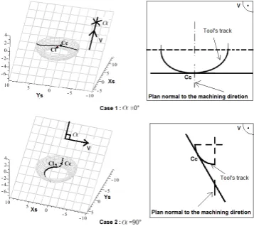
The object of this study is to propose a global optimization method to minimize the machining time of free-form surfaces in 3-axis milling. A toric end mill with cutter radius R and torus radius r is used, with a strategy of parallel planes of type zigzag. Free-form surfaces present a set of curved zones, i.e. concave and convex zones. The geometry is obtained by serial paths of a tool to approach the theoretical shape. During machining, tool moves tangentially to the workpiece at the point Cc. At this point the tool can move in any
directionα. This parameterαis called feed motion direction. For example, on an inclined plane (30◦ slope), the (fig.1) presents two cases of movements of a toric end mill cutter (R=5 and r=2). The tool is partially presented by a quarter of torus. The Zs is the axis of tool. The bold line curve
[image:2.595.305.532.221.415.2]represents the trace left by the tool atCc (see section A).
Fig. 1. Trace left by the tool according to the feed motion direction.
In case 1 on fig.1 with feed motion direction (α = 0◦)
the direction of steepest slope, the trace left by the tool at Cc results in a curve with an important radius curvature at
Cc. Moving perpendicularly to the direction of steepest slope
(α= 90◦)atC
c, the trace left by the tool is equal to r. The
quantity of material removed during the tool path (α= 0◦)
is much more important than in(α= 90◦). Then the number of paths required to machining the surface with(α= 0◦)is inferior than the number of paths with(α= 90◦). Therefore the time required to machine the surface in case 1(α= 0◦)
is less than the machining time for the same surface in case 2 (α= 90◦).
The conclusion is that the choice of feed direction has an influence on the trace left by the tool on the surface. The more the radius of this trace is important and the more the time of machining decreases. The radius of curvature of the trace left by the tool on Cc is called effective radius
Ref f. Our object is to use optimization method enabling us
to choose the optimal feed direction in different zones on the surface to minimize machining time.
A. The trace left by the cutter
The trace left by the cutter on the surface is the swept curve. Effective radius corresponds to the radius of curvature onCc of the swept curve projected in a plane normal to the
feed direction along a direction parallel to the feed direction. The toric end mill enables to keep a large effective radius while avoiding unsightly marks. [9] demonstrates that, in the point of contactCc, the effective radius is equal to the ellipse
radius -resulting from the projection along the feed direction in a plane normal to the feed direction of center-torus circle-increased by an exterior offset with a value equal to the torus radius of tool r. This gives us the analytical equation of the effective radius:
Ref f =
(R−r)cos(α−ϕCc)2
[image:2.595.47.226.354.513.2]sin(P)(1−sin(α−ϕCc)2sin(P)2)+r (1)
Fig. 2. Different angles of theRef f.
This analytical expression is easy to handle. It depends on the feed direction’s angleαbetween the feed rate−→V and the axis of the surfaceXs.
B. Step-over distance calculation
Step-over distance corresponds to the distance between two successive and parallel tool paths while respecting the maximal scallop heighthc (fig). 3. Sincehc is small (in the
order of 0.01mm) the following hypothesis are made:
• The tool makes a circular trace of radiusRef f in the
neighborhood ofCc.
• The radius of curvatureρof the surface is assumed to
be locally constant in a plane perpendicular to the feed motion direction.
• hc is small compared to Ref f andρ.
To calculate the step-over distance, in a plane perpendicular to the feed rateV~, eq.2. is obtained:
Pt=
s
8∗hc∗Ref f ∗(Ref f +ρ)
ρ (2)
Fig. 3. Step-over distance.
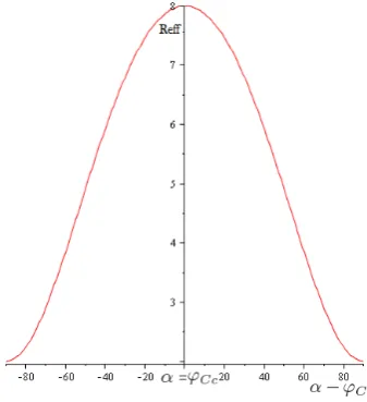
C. Influence of the feed direction on the effective radius
According to eq. 1, the effective radius is in direct relation to the feed direction α. In this section the impacts of this direction on the variation ofRef f is studied. Let (R=5 and
r=2) be torus end mill cutter, for an inclined plane (30◦ slope), the feed direction is varied in an angular interval of [−90◦,90◦]. The interest of moving the tool along the steepest slope direction(α=ϕCc)to maximize the effective radius is noted on fig. 4. For the whole surface, it’s not possible to do this because the steepest slope direction varies at any point, and in parallel planes strategy a constant machining direction is imposed.
Fig. 4. Variation of the effective radius of the torus end milling cutter.
III. APPROACH
The machining time is directly related to the feed direction of the tool. The analytical expression of this time is not known and by hypothesis it’s proportional to the length of the paths crossed by the cutter. To calculate the machining time, it’s necessary, from a first path, to define all successive paths
resulting to the minimal step-over distance from previous path. It’s a long computation which cannot be repeated if a quick answer is wanted. Minimizing the time of machining is equivalent to minimize the overall length of the path crossed by the tool. This is similar to maximize the step-over distance i.e. maximize the effective radius. So in our study the effective radius is taken as a parameter instead of time. Let S(u,v) be a parametric complex surface. At any point of this surface, there is an optimal feed direction corresponding to the steepest slope direction. Machining the surface with a single feed direction cannot guaranty the maximum effective radius at any point, because of the variation of the normal direction on the surface. Indeed, an optimal feed direction for one point of a path can be very far from an optimal feed direction for another point of the same path. It induces contraction of parallel planes distance and decreases the average value of the effective radius.
For this, the surface is mapped with a parametric meshing following (u,v). Each mesh presents a simple quadrilateral surface, with a low variation of the normal and an optimal feed direction.
The computation of an optimal feed direction on a mesh is as follows:
• Select a set of points on the mesh i: nbpi. This
selec-tion is done uniformly over the rows and columns of the mesh i by respecting distance fixed between two adjacent points, on fig.6 an example with nbpi=16 is
presented.
• Calculate for each point j: slopeP and steepest slope directionϕCc.
• Calculate the optimal feed directionαfor all points of a
mesh i maximizing the function:M axPnbpi
j=1 Ref f(j)=
M ax
nbpi
X
j=0
( (R−r)cos(α−ϕCc) 2
sin(P)(1−sin(α−ϕCc)2sin(P)2)+r)
(3) Each mesh is characterized by an optimal feed direction for which the sum of effective radius is maximized. A zone is a composition of a set of associated meshes. Two meshes can be associated if they are contiguous, meaning that they have at least one side in common. If the cross time of the tool from zone A to zone B, is negligible, the optimal solution to machine a mapped surface is to machine each mesh indepen-dently following its optimal direction, maximizing thereby the sum of effective radius of the surface. But since this approximation is not acceptable therefore the meshes of the surface are combined in zones. In order to have a sum of the effective radius of each zone superior to the sum of effective radius of each meshes composed the zone multiplied by a penalty:Pk(bnm) = ((SRef f(i)+SRef f(j))∗Pk(bnm))<
SRef f(Zij). The object is to maximize the sum of effective
radius of each zone. The penalty reflects the loss time due to the movement of tool from a mesh to another. To solve the problem a global optimization method is applied to constitute the zones:
• The number of zones should not be too large to avoid
the loss unproductive time of the tool.
[image:3.595.47.216.479.664.2]• Let M ={m, m2, ...mn} be a set of meshes covering
the whole surface.
• Let Z={z1, z2, ...zl} be a set of zone covering a set of
continguous meshes, withzi={mi...mp} ⊂Z, such
as the effective radius of zi is lower than the sum of
effective radius of all meshes {mi...mp} multiplied
by the penalty owed to the displacement of the tool.
• The set Z must cover all meshes of the set M: Pl
i=icard(zi) =card(M).
The problem to maximize the sum of effective radius is compared to the multi-Vehicle Routing Problem (mVRP). mVRP is a class of operational research and combinatorial optimization. A series of routes starting from a single depot are determined, based on a list of cities with a fleet of ho-mogeneous vehicles, in order to minimize the total distance traveled by the vehicles. Usually, a constraint limiting the total duration of the route [10] is added. The object is to visit all cities by minimizing one or several criteria related to the cost of delivery demands. It’s a classical extension of Travelling salesman problem and it belongs to the NP-difficult problem’s category [11][12][13].
The commonalities between the mVRP and the machining problem are:
• In mVRP a vehicle visites a set of defined cities. In machining problem a tool machined a set of defined meshes.
• In mVRP the necessary number of vehicles to visit all cities is found. In machining problem the number of required zones to cover all meshes is found.
• In mVRP one city is visited only once. In machining
problem one mesh is machined only once.
In this study, the order of the machining of zones is not considered contrary to the mVRP.
IV. OPTIMIZATION
To solve machining problem, Clarke and Wright’s opti-mization algorithm [14] used for solving mVRP is adapted. Clarke Wright’s algorithm (CW): developed by Clarke and Wright (1964), is one of the known heuristic for solving constraints vehicle routing problem [14]. CW is based on the notion of saving. Initially, a feasible so-lution consists of N back and forth routes between the depot and a customer. At any given iteration, two routes
(v0, ...vi, v0)and(v0, vj, .., v0)are merged into a single route (v0, ..., vi, vj...., v0) whenever this feasible, thus generating
a saving:Gi,j=C0i+C0j−Cij,C0i cost moving between
the depot 0 and city i.
Its concept is to link the routes determined by the savings list in which values are sorted from largest to smallest.
There are two versions of CW: sequential and parallel. Sequential version, a single route is expanded until no more routes can be linked to it. In the parallel version, several routes can be constructed in parallel. In the parallel version of the algorithm, the combinaiton of routes with the largest saving is always implemented, whereas the sequential version keeps expanding the same route until this is no longer feasible. In the practice the parallel version is much better [15].
The parallel version of CW algorithm is used in this study. The initial solution is to machine each mesh individually with
the optimal feed direction and maximum sum of effective radius. To calculate the optimal feed direction the eq.3 is used according to the number of points selected in each mesh. The sum effective radius of mesh i,SRef f(i), is equal to the sum
of effective radius of the selected points in this mesh for an optimal feed direction calculated.
Gi,j =SRef f(Zij)−((SRef f(i)+SRef f(j))∗Pk(bnm))
(4) With:
• Pk(bnm) penalty of tool’s movement between mesh i
to the mesh j.
• Zij: zone composed with meshes i and j.
The penaltyPk(bnm)is a linear function depending on the number of meshes in zones to be combined. The combination of meshes is performed if and only ifGi,j >0.
Pk(bnm) =k+(1−k)
(n−1)∗(bnm−1), k∈[0.9,1] (5)
There are three constraints: connecting meshes in the zone, belonging mesh to a single zone and zones covering the whole surface.
V. APPLICATION TO AN EXAMPLE
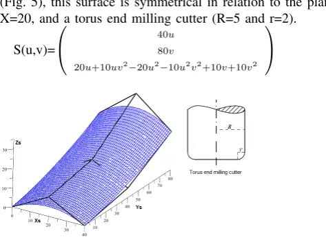
Let S(u, v) be a parametric free-form surface defined by (Fig. 5), this surface is symmetrical in relation to the plane X=20, and a torus end milling cutter (R=5 and r=2).
S(u,v)=
40u
80v
[image:4.595.304.541.369.545.2]20u+10uv2−20u2−10u2v2+10v+10v2
Fig. 5. Free-form surface S (u,v).
This surface has large variations in steepest slope direction, going from14◦ to166◦. Machining the surface with a single feed direction may induce areas with effective radius equal to torus radius r.
CW algorithm is not an exact optimization method. To approximate the solution of our problem to the optimal solution, the surface S(u,v) is mapped with parametric grid
3*3following (u,v), i.e. surface is covered by grid composed of nine meshes. In each mesh 16 points are selected. In order to verify the convergence of the CW algorithm to the optimal solution, in the first time, all possible combinations of these nine meshes are calculated and this SRef f(i) is evaluated.
One combination corresponds to a set of zones covering all surface’s mesh. The number of combinations obtained is 656. Global optimal solution Solopt with maximal sum
{0,1,2},{3,4,5}et{6,7,8}(see fig.6. to the numbering of the meshes).
In the second time, the CW algorithm is applied. The initial solution is to machine each mesh i individually with αopt(i). So the global effective radius of surface is
equal to the sum of the effective radius SRef f(i) of the 9
meshes multiply by the penalty:SRef f =P 8
i=0SRef f(i)= 1215.90mm. The disadvantage is the loss of time generated during the tool’s movement from a mesh to another one.
Fig. 6. The mapping of surface S(u,v).
The adjacency matrix of the meshes is given as follows:
M(u,v)=
0 1 0 1 0 0 0 0 0
1 0 1 0 1 0 0 0 0
0 1 0 0 0 1 0 0 0
1 0 0 0 1 0 1 0 0
0 1 0 1 0 1 0 1 0
0 0 1 0 1 0 0 0 1
0 0 0 1 0 0 0 1 0
0 0 0 0 1 0 1 0 1
0 0 0 0 0 1 0 1 0
The order between two adjacent meshes is not important. For example, the combination of mesh i and mesh j is the same than the combination of mesh j and mesh i.
The example below explains the calculating of sum of effective radius SRef f(0) for mesh 0 in the surface S(u,v).
Let (0,0), (0, 0.33), (0.33,0) et (0.33,0.33) be the (u,v) coordinates of mesh 0. The table presents four selected of the 16 existing points in the mesh 0.
TABLE I
THE CALCULATION OF THEPj(◦)ANDϕCcj(◦).
Point j Coordinates of point j Pj(◦) ϕCcj(
◦)
0 (0.041,0.041) 25.22 16.05
1 (0.041,0.125) 25.80 18.34
2 (0.041,0.208)) 26.36 20.63
3 (0.041,0.291) 26.94 20.63
Optimal feed direction is calculated by eq.3.:αopt=29.80◦.
Sum of effective radius of mesh 0 is: SRef f(0) = P
16 j=1(
(R−r)cos(αopt−ϕCcj)2
sin(Pj)(1−sin(αopt−ϕCcj)2sin(Pj)2) +
[image:5.595.302.551.80.143.2]r) = 169.918mm.
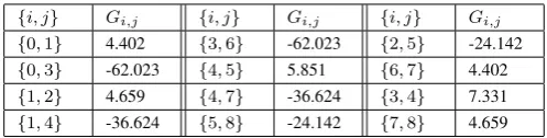
Table 1 presents the savingGi,jof the all combinations of
adjacent meshes in pairs according to the adjacently matrix M(u,v). Gi,j = ((SRef f(i)+SRef f(j))∗P0.98(bnm))−
SRef f Z(i,j).
Calculation example ofG0,1of the S(u,v) with 16 points:
• SRef f(0)= 169.918andSRef f(1) = 146.788.
• k=0.98.
• Total number of meshes of surface is n=9.
TABLE II SAVINGGi,j.
{i, j} Gi,j {i, j} Gi,j {i, j} Gi,j
{0,1} 4.402 {3,6} -62.023 {2,5} -24.142
{0,3} -62.023 {4,5} 5.851 {6,7} 4.402
{1,2} 4.659 {4,7} -36.624 {3,4} 7.331
{1,4} -36.624 {5,8} -24.142 {7,8} 4.659
• The combination is made between two meshes 0 and 1: bnm= 2.
• ThenPk(bnm) = 0.98 +
(1−0.98)
(9−1) ∗(2−1) = 0.982.
• To calculate the effective radius of a combination of mesh 0 and 1, on all points of the two meshes: 32 points (16 for each mesh)SRef f(Z0,1)= 315.567mm.
• Saving G0,1 = 315.567 − ((169.918 + 146.788) ∗ 0.982) = 4.402mm.
In table 1, negative saving means that the combination of mesh engenders a time loss. The positive saving is selected in ascending order.
• The first combination with a maximum savingGi,j is:
the mesh 3 and 4, forming zone Z0=>(SRef f(Z0) = 418.956, α0= 90). To respect the constraint of
unique-ness of belonging a mesh in a zone, all combinations containing mesh 3 or 4 are eliminated , i.e.:{0,3} {1,4} {3,6}{4,5} {4,7}.
TABLE III
SAVINGGi,jAFTER THE CREATINGZ0
{i, j} Gi,j {i, j} Gi,j {i, j} Gi,j
{0,1} 4.402 {3,6} eliminate {2,5} -24.142
{0,3} eliminate {4,5} eliminate {6,7} 4.402
{1,2} 4.659 {4,7} eliminate {3,4} Z0
{1,4} eliminate {5,8} -24.142 {7,8} 4.659
• Among remaining combinations, the maximum saving isG1,2, Z1=>(SRef f(Z1)= 274.195, α1= 39.72).
• Last combination with positive saving is G7,8, Z2 => (Ref f(Z2)= 274.195,α2= 140.28).
The formation of these three zones Z0, Z1, Z2 is done
in parallel and three meshes remains uncombined 0, 5, 6. The process is reiterated until all savings are negative. After several iterations of the program, the following results are obtained:
• Zone Z0, consisting in meshes 3, 4 and 5 => (SRef f(Z0)= 569.837, α0= 90).
• Zone Z1, consisting in meshes 0, 1 and 2 => (SRef f(Z1)= 442.044, α1= 35.68).
• Zone Z2 consisting in meshes 6, 7 and 8 => (SRef f(Z2)= 442.044, α2= 144.32).
• Sum effective radius of surface is
P2
j=0(SRef f(Zj)) = 1368.422mm (with penalty of
moving tool).
The solution obtained by CW algorithm is equal to the global optimal solution in taking into account the penalty, Solopt=1368.422mm. The application of the CW algorithm’s
on the mapped surface S(u,v) with parametric grid 3*3
converge to an optimal global solution.
Fig. 7. Machining of S(u,v) with three zones.
TABLE IV
MACHINING OFS(U,V)WITH SINGLE ZONE.
αopti(◦) SRef f
90 1034.962
TABLE V
MACHINING OFS(U,V)WITH THREE ZONES.
ZoneZi αopt(i)(◦) SRef f(i)
Z0 90 569.837
Z1 35.68 442.044
Z2 144.32 442.044
SRef f=1368.422
According to the two tables, during the machining of the surface on three zones a saving of 24.36% on sum of effective radius on overall surface is found compared to machine surface with single optimal feed direction. Indeed, during machining with single optimal feed direction, there are zones with important effective radius superior to R and other with low effective radius penalizing sum effective radius. This variation is due to the large variation in the slope of the surface, [14◦,166◦]. Slope is a fixed parameter that cannot be manipulated. It depends on the structure of the workpiece. When the surface is machined into three zones, an optimal feed direction is chosen according to the variation of slope in the zone. The sum of effective radius is maximal and homogeneous in each zone. It contributes to maximizing the distances between paths i.e. minimize machining time.
Machining time is not a linear function according to the effective radius because of the technical considerations taken into account such as positioning of the workpiece on the machine and machine’s dynamic. Time saving obtained by machining in three zones is 32.48 % compared to the machining in one zone with same technical constraints.
VI. CONCLUSION
In this paper, the optimization of 3-axis milling time of free-form surface is studied. For this, a toric end mill and strategy by parallel planes of type zigzag are used. The effective radius is calculated by analytical equation and the relation between this effective radius and step-over distance is established. When the step-over distance increase the effective radius increase generates a decreasing of the machining time. Our object is to minimize the machining
time, but the analytical expression of the time is not known, then the sum of effective radius is taken as a parameter instead of time. One of the parameters influencing the sum of effective radius is the feed motion direction. Machining the free-form surface with a single direction cannot guaranty the maximum effective radius in any point because of the large slope variation on the surface. That gives the zones with low effective radius penalizing the sum of effective radius on the whole surface. To get an optimal feed direction at any point this study is interested in machining with zones. The analysis of complex surface as a set of simple sub-surfaces simplifies the global problem. This enables to calculate the optimal feed motion direction for each sub-surface then minimizing the machining time taking account the increase of cross time between zones by penalty coefficient. After decomposition of the surface in meshes, the Clarke and Wright’s algorithm is used to combine meshes in zones and reduce the movements’ cost of time. The results obtained on the presented workpiece show a significant reduction of machining time.
The future works aspire to study minimization of the machining time of the free-form surfaces by zones using optimization methods taking into account kinematic and dynamic behavior of the machine.
ACKNOWLEDGMENT
This work has been partially supported by French National Research Agency (ANR) through the COSINUS program under the grant ANR-09-COSI-005.
REFERENCES
[1] I. D. Faux and M. J. Pratt,Computational geometry for design and manufacture. Halsted Press, 1985.
[2] K. Marciniak, “Geometric modelling for numerically controlled ma-chining author: Krzysztof marciniak, publisher: Oxford university press,” 1992.
[3] Y. Huang and J. H. Oliver, “Non-constant parameter nc tool path gen-eration on sculptured surfaces,”The International Journal of Advanced Manufacturing Technology, vol. 9, no. 5, pp. 281–290, 1994. [4] B. Kim and B. Choi, “Guide surface based tool path generation in
3-axis milling: an extension of the guide plane method,”Computer-Aided Design, vol. 32, no. 3, pp. 191–199, 2000.
[5] G. C. Loney and T. M. Ozsoy, “Nc machining of free form surfaces,”
Computer-Aided Design, vol. 19, no. 2, pp. 85–90, 1987.
[6] S. T. Peternell M., Pottman H. and Z. H, “”swept volumes”,”Computer aided design, vol. 2, no. 5, pp. 599–608, 2005.
[7] Z. Chen, G. Vickers, and Z. Dong, “Integrated steepest-directed and iso-cusped toolpath generation for three-axis cnc machining of sculptured parts,”Journal of manufacturing systems, vol. 22, no. 3, pp. 190–201, 2003.
[8] H. Y. Maeng, M. H. Ly, and G. W. Vickers, “Feature-based machining of curved surfaces using the steepest directed tree approach,”Journal of Manufacturing Systems, vol. 15, no. 6, pp. 379–391, 1996. [9] J. Senatore, S. Segonds, W. Rubio, and G. Dessein, “Correlation
between machining direction, cutter geometry and step-over distance in 3-axis milling: Application to milling by zones,”Computer-Aided Design, 2012.
[10] G. B. Dantzig and J. H. Ramser, “The truck dispatching problem,”
Management science, vol. 6, no. 1, pp. 80–91, 1959.
[11] N. Christofides, A. Mingozzi, and P. Toth, “The vehicle routing problem,”Combinatorial optimization, vol. 11, pp. 315–338, 1979. [12] J. K. Lenstra and A. Kan, “Complexity of vehicle routing and
scheduling problems,”Networks, vol. 11, no. 2, pp. 221–227, 1981. [13] M. W. Savelsbergh and M. Sol, “The general pickup and delivery
problem,”Transportation science, vol. 29, no. 1, pp. 17–29, 1995. [14] T. Pichpibul and R. Kawtummachai, “New enhancement for
clarke-wright savings algorithm to optimize the capacitated vehicle routing problem,”European Journal of Scientific Research, vol. 78, no. 1, pp. 119–134, 2012.