Exploiting user behaviour for contextaware power management

Abstract— With more and more computing devices being deployed in buildings there has been a steady rise in buildings' electricity consumption. At the same time there is a pressing need to reduce overall building energy consumption. Pervasive computing could further exacerbate this problem but it could also provide a solution. Context information (e.g., user location) likely to be available in pervasive computing environments could enable highly effective device power management. The objective of such context-aware power management (CAPM) is to minimise the overall electricity consumption of a building while maintaining acceptable user-perceived device performance.

To investigate the potential of CAPM we conducted experimental trials for two simple location-aware power management policies. Our results highlight the presence of two distinct user behaviour patterns but also show that location alone is not enough for effective power management.

We therefore propose a CAPM framework that employs Bayesian Networks to support prediction of user behaviour patterns from multi-modal sensor data for effective power management. We further propose the use of acoustic data as an interesting context for predicting finer-grained user behaviour. The paper presents an initial evaluation of the resulting framework.

Index Terms— Context-aware, power management, user behaviour, Bayesian Network.

I. INTRODUCTION

With more and more computing devices being deployed in buildings there has been a steady rise in buildings' electricity consumption [1], [2]. These devices not only consume electricity, they produce heat, which increases loading on ventilation systems, further increasing electricity consumption. At the same time there is a pressing need to reduce overall building energy consumption. The European Union's strategy for security of energy supply highlights energy saving in buildings as a key target area [3]. Pervasive computing will potentially further increase the number of computing and sensing devices in buildings. A key question is how will this affect electricity consumption? In particular, what we are interested in is whether user context (derived from pervasive computing) can enable highly effective power management of stationary devices to significantly reduce buildings’ overall electricity consumption.

Dynamic power management [4] is a powerful technique for reducing device power consumption by taking advantage of idle periods during the operation of the device. The two fundamental assumptions are (i) idle periods will occur during

the device's operation and (ii) these periods can be predicted with a degree of certainty. What makes dynamic power management difficult is the fact that for most devices power state transitions have a significant cost. Typically a power state transition may consume extra energy (e.g., spinning up a hard disk), reduce device performance (e.g., a user waiting for a monitor to wake up) and possibly reduce its lifetime (e.g., fluorescent light bulbs burning out). Therefore not all idle periods are long enough to justify powering down the device. The primary task of the power management policy is to predict (based on past information) whether the current idle period will be long enough (i.e., greater than the breakeven time) to justify the transition cost. Secondarily, if the policy can predict when the next user request will be made it can reduce the time the user is waiting for the device to wake up.

Most current research in dynamic power management is applied to extending battery life for mobile devices with some research beginning in the area of power management for servers and server farms [5], [6]. The majority of policies are device-level and they concentrate on management of sub-components within the computing device, either the hard disk, processor, memory or network card. More advanced policies use information from higher up in the system to make more intelligent power management decisions.

To develop effective user-level policies for stationary devices we need to obtain context from the user of the device, in particular when the user is ‘not using’ the device (for longer than the breakeven time) and when the user is ‘about to use’ the device (the resume time beforehand). Determining this user context is the most challenging part of CAPM and there is a balance between how much energy additional context can save and how much it will cost both monetarily and energy wise.

Section II discusses two recent papers that address CAPM. We then present results from experimental trials of two simple location-aware policies in Section III. The results highlight two distinct user behaviour patterns but also show that location alone is not enough for effective CAPM. The more clues we have of the user’s behaviour in the space the better we can power manage the devices. Section IV presents some requirements derived from the results and an initial design of the CAPM framework. Finally, Section V gives an initial evaluation of the resulting framework and Section VI concludes.

Exploiting User Behaviour for Context-Aware

Power Management

Colin Harris and Vinny Cahill

II. RELATED WORK

We analysed two research papers that specifically examine using context to manage power of devices in an environment. We evaluated these CAPM solutions based on (i) the energy cost of the system, (ii) the potential energy savings and (iii) the user-perceived performance.

A. Location Aware Resource Management in Smart Homes

The MavHome project’s goal is the creation of an intelligent home environment [7]. The paper [8] focuses on resource (power) management of the electrical devices in a home environment. Their example floor plan (see Fig. 1) is divided into 15 zones containing 11 RFID readers and 9 pressure mats. Zone connectivity is represented as a simple graph with each edge of the graph containing a list of the sensors a user would pass to get from one zone to the next. These are termed “paths” and there may be more than one path between zones. Zones and sensors are labelled alphabetically.

Fig. 1 MavHome sample floorplan (Source: [8])

The user’s symbolic location is determined by sampling the 20 sensors and user mobility is captured as a string of characters, for example, “ajlloojhhaajlloojaajlloojaajlm”. This gives room-level location granularity with the use of pressure mats to divide up the large open plan kitchen, dining, and living rooms. There are two parts to their CAPM algorithm:

1. When the user leaves a zone, predict the path to the next zone based on their current zone and the user’s mobility history.

2. Switch on all devices along the path. (We assume that all devices in the previous zone are switched off after a short timeout period.)

Emphasis is given to the user mobility part of the algorithm. The Lempel-Ziv text compression scheme is used to compress user mobility strings, which are subsequently sent to a server and stored in a search trie. This reduces the cost of data acquisition but delays the propagation of the user’s location potentially causing large delays in power management of devices. The mobility prediction scheme makes its decisions based solely on the history of room-level user mobility and does not take into account other valuable data such as the time-of-day or day-of-week to aid its prediction.

The power management decision to switch on all devices in the user’s predicted path from one zone to the next is naïve. First, they do not categorise the devices into “continuous” and “intermittent” devices. Continuous devices experience no idle periods during their operation and typically they are devices that carry out a well-defined task such as making coffee, cooking food, washing clothes etc. Only intermittent devices (i.e., devices that experience idle periods) are suitable for context-aware power management. Intermittent devices include lighting, sound, video display, heating, cooling and ventilation. Second, a user will typically not require all intermittent devices all the time. Switching on all of these devices all of the time will potentially frustrate the user and waste energy.

We estimated the energy consumption of the devices that comprise the MavHome IT infrastructure. Where possible power estimates have been measured, otherwise they have been derived from manufacturers’ datasheets. We assume the IT system runs 24 hours per day. The estimated daily energy consumption of the system is 8 kiloWatt hours (kWh). If we consider the network to be an existing infrastructure providing many other services then we can attribute the energy consumption of the location sensors to the energy cost of the CAPM system. This alone consumes 2.5 kWh per day, which is 30% of the total IT system.

The total power of all domestic devices is 10.5 kW and estimated daily energy consumption is 17.7 kWh. We estimated the number of usage hours based on a not very energy conscious user. All intermittent devices are left on when awake and in the house (i.e., 7am to 9am and 6pm to 12am). Usage of task specific continuous devices has also been estimated. Fig. 2 shows that location sensing consumes up to 10% of the total energy consumption with only a potential to save an estimated ½ of the 37% through more efficient management. The system just breaks even bringing into question its practicality.

21%

10%

32% 37%

IT infrastructure

Location sensors Continuous devices Intermittent devices

Fig. 2 MavHome energy consumption

is not the case. Mozer cites even a 700ms delay in his system is enough to annoy the user [10]. Second, the path prediction success is 85% meaning 15% of time the predictive policy will switch on the wrong set of devices and the user will be left to manually switch these off and the desired ones on. For the system to be workable we believe the predictive success has to be close to 100% to avoid user annoyance. Probably the most fundamental flaw is assuming the user will want all devices in their future path switched on. There is no mechanism for capturing the user’s preferences. A simple improvement to the policy would be to only switch on the devices that had been on the last time the user was in the room.

B. Lessons from an Adaptive House

The Adaptive House project [9] has a similar floor plan and device energy consumption to the MavHome project but has a more sophisticated CAPM framework that has been developed from 8 years of actual implementation and experimentation. The real life experience from this project highlights the subtle requirements for effective power management. Here user mobility prediction is only one component of their CAPM framework and they utilise dozens of environment and user context variables in making their power management decisions. Also, the project focuses only on “home comfort” devices, namely air temperature, water temperature and lighting devices. These devices fall into the category of intermittent use.

The system is composed of 75 sensors monitoring room temperature, ambient light, motion, sound level, door and window positions, and outside weather and insolation. Actuators control a central heating furnace, electric space heaters, water heating, lighting and ventilation. [10] concentrates on the issue of lighting control, the objective being to automate the setting of lighting levels within the house to maximise inhabitant comfort and minimise energy consumption. The main challenges are:

1. There are several lights in each room, each with 16 settings. The user prefers different lighting moods depending on the task s/he is doing.

2. Motion sensors have a time lag in detecting user occupancy and there is delay in the X10 comms of 700ms causing a delay in system response.

3. Motion sensors detect the presence of a person well, but they do not detect their absence. A person could still be in the room reading but not moving.

4. The policy must satisfy two often opposing constraints, user comfort and energy consumption. The lighting control system architecture is shown in Fig. 3 below.

Fig. 3 Adaptive House Architecture (Source: [10])

It has two levels of abstraction that filter noisy sensors and provide higher-level information to the Q-learning controller. This reinforcement learning technique models user discomfort and energy costs and uses trial and error learning to minimise the total average cost. The implementation has a partial model of the environment (It can learn about other “bad decisions” in lighting level based on the setting the user selects. If the decision was A and user corrected up to C, then any B lower than A would also have been a “bad decision”).

The natural light estimator estimates natural daylight from raw sensors (as if the lighting was turned off). The anticipator is a neural network that predicts if a zone will be entered in the next 2 seconds. It runs every 250ms and inputs are motion, door status, sound level, zone occupancy and time of day. This component has been identified as not predicting sufficiently accurately due to sparse sensor representation. This caused user annoyance when lights would go on in an unoccupied zone. The occupancy model predicts whether a zone is occupied or not and the inputs are motion sensed in zone, number of people in house and motion in adjacent zones. The state estimator forms a high-level state representation for decision-making with the most important inputs being estimated user activity and natural light level. The user’s activity is determined by zone change frequency.

We estimated the energy consumption of the IT system including the sensors, power supplies, conditioning boards and X10 lighting device actuators to be 4 kWh. The power of the sensor system was difficult to estimate, as full details of the actual hardware implementation was not known. However, our current estimate envisages the sensor equipment consuming up to 0.8 kWh, which is 20% of the IT system.

14% 4%

35% 47%

IT infrastructure

Sensors/Actuat ors

Continuous devices Intermittent devices

Fig. 4 Daily energy consumption for non-energy conscious user

The Q Learning policy costed energy ($0.072 per kWh) and user discomfort ($0.01 per manual adjustment, $0.01 per failed anticipation and $0.01 per false turn on) in dollar units and graphed these costs over time. Fig. 5 shows the “energy cost per event” dropped over time from 0.5 cent to 0.05 cent. However, it is not clear how this cost relates to the actual energy cost of the lighting. The graph also shows the user discomfort cost starting at 0.1 “cent per event” rising to 0.8 and decreasing again to 0.01 cent per event (after an error in the system code was fixed).

Fig. 5: Energy versus user discomfort (Source: [10])

These figures do not really give a good idea of the user-perceived performance. The two main “discomforts” the author experienced were the slow response of the system (due mainly to X10 communication delay) and the occasional false anticipation of zone entry. This caused switching of lights on in unoccupied zones. Surprisingly, there is no specific evaluation of the control of lighting level based on user activity prediction. User activity is based only on recent user mobility patterns. For example, the user being still for 5 minutes equates to “user reading” and frequent zone change equates to “cleaning house”.

C. Conclusions

The Adaptive House system is quite advanced and benefits from actual implementation and real experimental trials. However, neither of the papers give a clear model or measurement of the environment’s overall power consumption, which we believe is necessary in fully evaluating the effectiveness of CAPM.

Finally, Mozer notes that user activity (behaviour) classification is an interesting area of future research. This suggests the control of lighting level based on user activity prediction needs further work.

III. INITIAL EXPERIMENTAL RESULTS

To explore further the requirements of context-aware power management and gain insight into user behaviour patterns, we examined in detail the power management of users’ stationary desktop PCs in an office environment. The objective was to minimise overall electricity consumption of the system while maintaining acceptable desktop PC performance. In particular, we evaluated the use of location as a key piece of context for CAPM. We are interested in the relation between the user’s location and their user behaviour (i.e., whether they are using the device or not). We implemented two simple location-aware policies and performed 6 user trials, each over a period of a week. The trace data collected from the trials was analysed to gain insight into the energy consumption and user-perceived performance of the location-aware policies.

The office spaces included personal and shared spaces, and there was only one user per desktop PC. The two simple location-aware policies use the location context derived from detecting users’ Bluetooth-enabled mobile phones. A power manager service executes on each desktop PC and continuously polls to discover Bluetooth devices in the area.

Figure 6 PC polls to discover Bluetooth-enabled mobile phones

The two location-aware policies were:

down to standby, when it resumed to the on state, both automatically and manually, and when the PC was on but idle for the last minute. This on-idle time enables us to estimate how much energy the policy wasted by the machine being on but (potentially) not being used. Knowing the idle times enables us to generate the “oracle” policy trace and the range of threshold policy traces. The oracle policy [11] is a theoretically optimal policy, which has future knowledge of user requests for the device. The threshold policy [12] is a simple policy that powers the device down after the given threshold idle period has elapsed.

The range of the Bluetooth connection is 10 metres and its latency is approximately 10 seconds (i.e., it can take up to 10 seconds for the Bluetooth inquiry to find the phone). We also noted during implementation that sometimes the inquiry would not find the phone even though it was there. To overcome this source of error it was necessary to duplicate the number of inquiries. This polling process takes approximately 90 seconds to complete so there is a significant delay before the machine is powered down.

Policy traces were collected from 6 separate user trials, 4 of which used the SOB policy and 2 of which used the SWOB policy. Software was written for analysing the traces in terms of energy consumption and user perceived performance. For each trace collected, the oracle policy trace and a range of threshold policy traces were generated. Also, for the SWOB policies, corresponding SOB policy traces were generated.

We estimated the mobile phone consumes an extra 6 Watt hours (Wh) of energy over the 4-day trial due to extra recharging necessary because the Bluetooth discover mode was on all the time. The extra energy consumed on the PC by the power manager was not measurable and we have considered it negligible. Also, for the SWOB policy we do not take into account the energy consumed by the wake up server, as we assume this functionality will be provided in the near future within the USB Bluetooth adapter. The 6 Wh has been added to the energy cost of the location-aware policies.

A. SOB policy energy performance

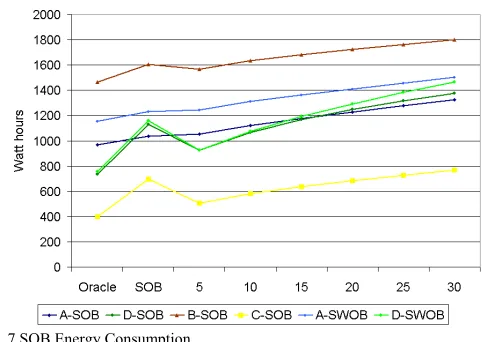
Fig. 7 below graphs the energy consumption in Watt hours for each policy for each policy trace. The SOB policy values are the actual estimated consumption from the real trace (except for A-SWOB and D-SWOB) and the other values are calculated from the generated policy traces. The traces are all the same length of 4 days, Tuesday to Friday. Each user has different user behaviour, which affects the performance of the policies. Previous monitoring of policy traces and actual measurement of PC power consumption show that, on average, the estimated power consumption (from the trace) correlates well with the measured power consumption (within 7.2% over a period of a week).

Fig. 7 SOB Energy Consumption

From the graph, it seems that there are two distinct user behaviour patterns (or limits) emerging. The SOB policy performs quite well for the A-SOB, A-SWOB and B-SOB traces (HeavyUsePattern). In these cases the SOB policy is close to the oracle policy (~8% from oracle) and similar in consumption to the Threshold-5 minute policy. The reason for the good performance is that A and B are heavy users of their PC while in its vicinity (i.e., the usage traces have a relatively small amount of idle time when the user is in the 10-metre vicinity).

The SOB policy performs similarly badly for the D-SOB, D-SWOB and C-SOB traces (LightUsePattern). In these cases the SOB policy is far from the oracle (> %50) and the traces have a significant amount of idle time when the user is in the 10-metre vicinity. We can state as a general rule, the SOB policy will perform well for devices that are heavily used when the user is in their vicinity.

Another pattern to note within the traces is the slope of the threshold policies’ consumption. The A-SOB, A-SWOB, B-SOB and C-B-SOB traces threshold consumption slopes are very similar (10.8, 9.3, 10.3, 10.5) (LowFrequencyUsePattern) compared to the slope of the D-SOB and D-SWOB threshold consumptions (18.0, 21.6) (HighFrequencyUsePattern). This indicates another distinct user behaviour pattern in the traces that affects the performance of the threshold policies. Intuitively, the higher the user’s frequency of idle periods the worse the threshold policy performs from oracle as it consumes extra power waiting to timeout, each time there is an idle period. So while the SOB policy performs badly for all three LightUse user traces, due to the large quantity of idle period time, the threshold policies perform worse for D-SOB and D-SWOB than C-SOB as user D has a high frequency of idle periods (41 and 47 periods) compared to user C (24).

B. SOB policy user perceived performance

period compared to the LightUse traces (11, 12, 14). As would be expected the performance improves as the threshold increases, with 20 minutes appearing to reach saturation (i.e., after this threshold there is little improvement in performance). What is interesting to note is that for the HeavyUse traces, the SOB policy performs similarly to the Threshold-5 policy but for the LightUse traces, the SOB performs considerably better. This intuitively makes sense, as the HeavyUse users do not allow the Threshold-5 policy to power down while in the office, whereas the LightUse users would. So, another general rule is that the SOB policy keeps the user-perceived performance acceptable for LightUse users.

Fig. 8 SOB User Performance

A qualitative survey of the users revealed that for 2 of the users the performance penalty of resuming the PC every time they came back to their office would not stop them implementing the SOB policy. The other 2 users thought it necessary that the PC would resume automatically to avoid the performance penalty. Clearly user-perceived performance is subjective and there is a balance for each user of how long the standby period should be to justify the subsequent performance penalty (i.e., a performance break-even time).

Fig. 9 shows the standby period frequency in minutes for the SOB and Threshold-5 policies for the D-SOB (LightUse) trace. The graph shows the Threshold-5 policy has many more short standby periods. Also, the total number of standbys for the SOB policy is 24 compared to 52 for the Threshold-5 policy. Therefore, 28 of the Threshold-5 policy standbys occurred when the user was in the vicinity. Clearly, these short standby periods when the user is in the vicinity would severely degrade the user-perceived performance, making the Threshold-5 policy unlikely to be implemented by any user.

Fig. 9 Standby Period Frequency

C. SWOB policy energy performance

The SWOB policy is an extension to the SOB policy where the PC powers up again when the mobile phone is next detected in the 10-metre vicinity. For this reason we chose to evaluate the policy with just two user trials. Fig. 10 shows the policies’ energy consumptions for the A-SWOB and D-SWOB traces. The graph compares the SWOB policy to the generated oracle, SOB and threshold policy traces. Again, the two users have similar performance to their original traces with A-SWOB performing well and D-A-SWOB performing badly compared to the oracle. Also, again the slope of the threshold performances is similar to the original user traces. For A-SWOB the A-SWOB policy energy performance is very similar to the SOB policy but for D-SWOB it is significantly worse. The increase in energy consumption is caused by the SWOB policy automatically resuming the PC when the user enters the vicinity. Hence, the PC can be on and idle before the user requests its use.

Fig. 10 SWOB Energy Consumption

D. SWOB user perceived performance

On average the Bluetooth discovery takes ~10 seconds to discover the mobile phone and the desktop PC takes ~7 seconds to fully resume from standby. Therefore, under the SWOB policy it takes ~17 seconds from the time the user enters the 10-metre vicinity until the PC fully resumes, ready for use. To evaluate the user-perceived performance of the SWOB policy we have to determine whether the PC was resumed in time for the user. Fig. 11 shows the graph of auto-on-idle period frequency in seconds for both traces.

Fig. 11 Auto-on-idle period frequency in seconds

The graph shows the D-SWOB trace to have few short periods (3 periods < 8 seconds) compared to the number of longer periods (25 periods > 60 seconds). On the other hand the A-SWOB trace has relatively many short idle periods (10 periods < 8 seconds) compared to no periods greater than 60 seconds. This data suggests that user A experienced delays in waiting for the PC to fully resume and user D experienced relatively few delays. The length of the delay is partly dependent on the geographical layout of the user’s return path and how long it takes the user to return to their PC after they have entered the 10-metre vicinity. In general, the current Bluetooth discovery time makes the auto wake up of the PC borderline functional and very dependent on the user’s return path and their time to reach the PC. A more responsive sensor could improve the SWOB policies user-perceived performance and be less dependent on geographical layout.

E. Conclusions

The experimental user trials and subsequent policy trace analysis has highlighted several user behaviour patterns that affect the performance of the power management policies. The location aware SOB and SWOB policies perform well energy-wise for HeavyUse users where the device is used a lot when the user is in the 10-metre Bluetooth vicinity. For LightUse users they begin to deteriorate, consuming energy when the user is in the vicinity but not using the device. For FrequentUse users (i.e., the user uses the device many times during the day) the threshold policies deteriorate as energy is wasted every time the policy waits for the timeout period. The SOB and SWOB policies are less affected by this FrequentUse pattern, as the timeout period is less (90 seconds).

The user-perceived performance of the SOB policy appears to be acceptable to some users but not others. The performance remains constant for both HeavyUse and LightUse users while the Threshold-5 policy performance deteriorates significantly for LightUse users. The SWOB policy user-perceived performance is dependent on the geographical layout of the user’s return path and how long it takes for the user to return to their PC after entering the 10-metre Bluetooth vicinity. This makes it suitable for only some cases. Furthermore, the SWOB policy comes at a price in increased energy consumption, particularly in the case of LightUse users and unsuitable geographical layouts (e.g., where the user passes by the office within the 10-metre range). A further concern of implementing these policies is that of device lifetime. For many devices, switching them on and off affects their expected lifetime. We have estimated the break-even due to lifetime for a desktop PC to be around 1 minute [13]. Other devices have longer lifetime break-even times such as fluorescent lighting (~5 to 10 minutes) [14]. Fig. 12 shows a relatively large number of short standby periods occurring for all users. Policies may have to take device lifetime into consideration when making their power off decisions.

Fig. 12 Standby period frequencies (minutes)

IV. CAPM REQUIREMENTS AND BASIC DESIGN

prediction could overcome the problem of the latent Bluetooth sensing. Furthermore, there is a need for distant sensing of users and possibly recognition of user plans to predict longer future idle periods (for cases where the device breakeven time is an order of minutes). For example, given the results it would not be sensible to switch off fluorescent lighting every time the user leaves the room as this would cause premature failure. Finally, location context alone is not sufficient to determine detailed user behaviour necessary for effective CAPM. Further context is needed to predict (i) the user in the vicinity but not using the device and (ii) the user in the vicinity and about to use the device. Passing by the device but not going to use it is a special case of scenario (i). The second scenario will be difficult to achieve, as one key advantage of location is that it is a distant sensing device, which enables time for the device to resume before the user requests its use. Saving energy by switching off devices in the vicinity of the user will be difficult to achieve transparently.

The initial experimental location-aware polices used a simple rule-based design where, observed states are matched to power management actions. There is no learning of new rules based on usage and there is no representation of uncertainty, which is required in most real-world decision applications to account for incomplete and noisy data [15]. This design would not scale well to accommodate more contexts, as the rules would become increasingly complex making it successively harder to configure for each individual user.

Some form of AI-based learning technique was needed, which could cope with incomplete and noisy sensor data and continually learn from device usage history. Our process of selecting a suitable technique involved first determining whether CAPM is a supervised or unsupervised learning problem. We believe that CAPM is best cast as a supervised learning problem. The success of the decision to power-down or power-up the device can be easily measured. Therefore sometime after, the reward for each decision can be evaluated and attributed to the specific decision the policy made. The total reward for the policy is simply the sum of the individual rewards. An unsupervised or reinforcement learning technique could possibly be applied (as in Mozer) but this will inherently be a more heavyweight solution, and slower to learn. The specific technique we chose for modelling the CAPM problem is Bayesian Networks [16].

A Bayesian Network is a graphical model that enables causal domain modelling and computes probability or ‘belief’ of inferred data (query data) based on the available evidence (input data). The fundamentals of Bayesian Networks come from Bayes’ theorem, which states that the probability of a hypothesis h given some evidence e is equal to the evidence’s likelihood P(e|h) times the prior probability of the hypothesis P(h), normalised by dividing by the evidence’s probability P(e). P(h|e) = P(e|h)P(h)/P(e).

The advantages of Bayesian networks for CAPM are: 1. The graphical programming model is simple to

understand and modify by non-technical users.

2. The model naturally represents the causal modelling of the inferred data ‘Not Using’, ‘About to use’.

3. The policy decision and utility can be represented with the Decision Network extension. The utility is easily user configurable.

4. The model can be configured with prior distributions so it can make intelligent (conservative) decisions from the start.

5. The learning process is relatively simple and should continually improve with more data.

6. Bayesian Networks can solve up to 36 nodes with a tractable / lightweight algorithm.

One possible disadvantage of Bayesian Networks is that if the prior distributions are incorrect, they can adversely affect the learning of an optimal policy. We believe the causal modelling and estimation of prior distributions are reasonably intuitive for the CAPM domain and this extra domain knowledge will add to the power of the solution, increasing its accuracy and speed of learning.

The CAPM decision problem naturally divides into two policies, the power-down policy and the power-up policy. Fig. 13 details a possible Bayesian Decision Network for the power-down policy. The IsNotUsing and IsNotUsingLater nodes are the query nodes. The probabilities for these nodes are inferred from the state of the CurrentIdleTime, BluetoothPhone, AcousticSensor and TimeOfDay input nodes. From a causal modelling perspective, the state of the user IsNotUsing ‘causes’ the observed states of the input nodes. The decision to power down is made based on the utility of the decision and the probability of IsNotUsingLater. This node represents whether the user will request use of the device before the device’s breakeven time. The Utility node can be weighted to change the value of the policy’s decision.

Fig. 13 Power-down policy

The power-up policy is similar in structure to the power-down policy but has different inputs, BluetoothPhone and

V. EVALUATION METHODOLOGY

We have implemented an initial prototype of the CAPM policies using the Netica Bayesian Network tool [17]. We conducted a case-based evaluation of the CAPM policies using test cases to demonstrate implementation of a number of scenarios. The additional (non-location) contexts CurrentIdleTime, TimeOfDay and AcousticSensor enable the policies to cope with the following scenarios. When the user passes by the office door (in Bluetooth range) the policy does not switch on as no sound of door opening is detected in the room. When the user is in the vicinity but is talking and has not used the PC for a while, after a sufficient CurrentIdleTime the policy powers down the PC. When talking ceases the probability “About to use” increases and the PC is powered up. The requirement for distant sensing could be fulfilled by enabling power managers to communicate.

To evaluate the learning capability of the policies we simulated two distinct case-base sets of 25 samples each. Table 1 below lists part of this sample data.

TABLE 1: SAMPLE CASES

ID Current IdleTime Bluetooth Phone TimeOf Day Acoustic Sensor IsNotUsingLater

1 3 Found 10 Silent Using

2 4 Found 12 Silent Using

6 20 Found 20 Silent NotUsing

7 24 Found 13 Silent NotUsing

11 4 NotFound 19.2 Silent NotUsing 12 2 NotFound 13.2 Silent NotUsing 19 3 NotFound 14 Silent NotUsing

20 1 NotFound 16 Silent Using

21 15 Found 15 Talking NotUsing 22 16 Found 15.2 Talking NotUsing 25 13 Found 16.5 Talking NotUsing

The policy networks were initialised with prior probability distributions and tested against the test set of cases. The decision error-rate was high at 72%. The network was then trained with the separate training set of cases and the error-rate improved to 20%. The results show that a relatively small set of sample data can greatly improve the accuracy of the policies.

VI. CONCLUSIONS

There are two strong motivating forces for context-aware power management; the steady rise in buildings’ electrical energy consumption and the pressing need to reduce energy consumption. User context could potentially enable highly effective context-aware power management to significantly reduce buildings’ electrical energy consumption.

Our results indicate that user location alone is insufficient for CAPM and further context is needed to determine finer-grained user behaviour for effective power management. A simple acoustic sensor could potentially tell us many things about the user behaviour. Is the office quiet? Is someone talking? Did the phone ring? Are there many people talking? Where is the sound coming from? Is that the sound of the door

opening? However, processing this data will have a cost in both CPU cycles and hence energy consumed.

Finally, there is a need to evaluate the CAPM framework in real-world situations. This will include a concrete evaluation of power consumed by the total system in order to evaluate the potential energy savings.

REFERENCES

[1] K. Kawamoto, J. G. Koomey, B. Nordman, R. Brown, M. A. Piette, and A. K. Meier, “Electricity used by office equipment and network equipment in the u.s.” in Proceedings of the 2000 ACEEE Summer Study on Energy Efficiency in Buildings. ACEEE, 2000.

[2] R. Jain and J. Wullert, II, “Challenges: environmental design for pervasive computing systems,” in Proceedings of the 8th Annual International Conference on Mobile Computing and Networking. ACM Press, 2002, pp. 263–270.

[3] European Comission, “Towards a european strategy for the security of energy supply,” 2000. [Online]. Available: http://europa.eu.int/comm/energy transport/en/lpi lv en1.html

[4] L. Benini, A. Bogliolo, and G. D. Micheli, “A survey of design techniques for system-level dynamic power management,” IEEE Transactions on Very Large Scale Integration (VLSI) Systems, vol. 8, no. 3, pp. 299–316, June 2000.

[5] J. S. Chase, D. C. Anderson, P. N. Thakar, A. Vahdat, and R. P. Doyle, “Managing energy and server resources in hosting centres,” in

Symposium on Operating Systems Principles, 2001, pp. 103–116. [Online]. Available: citeseer.ist.psu.edu/chase01managing.html

[6] C. Lefurgy, K. Rajamani, F. Rawson, W. Felter, M. Kistler, and T. W. Keller, “Energy management for commercial servers,” IEEE Computer, vol. 36, no. 12, pp. 39–48, December 2003.

[7] “Mavhome smart home project.” [Online]. Available:

http://mavhome.uta.edu/

[8] A. Roy, S. K. D. Bhaumik, A. Bhattacharya, K. Basu, D. J. Cook, and S. K. Das, “Location aware resource management in smart homes,” in

IEEE International Conference on Pervasive Computing and Communications. IEEE, March 2003, p. 481.

[9] “Adaptive house project.” [Online]. Available:

http://www.cs.colorado.edu/ mozer/nnh/

[10] M. Mozer, Smart environments: Technologies, protocols, and applications. J. Wiley and Sons, November 2004, ch. 12, pp. 273–294. [11] T. Simunic, L. Benini, P. W. Glynn, and G. D. Micheli, “Dynamic

power management for portable systems,” in Mobile Computing and Networking, 2000, pp. 11–19. [Online]. Available: citeseer.nj.nec.com/article/simunic00dynamic.html

[12] F. Douglis, P. Krishnan, and B. Marsh, “Thwarting the power-hungry disk,” in USENIX Winter, 1994, pp. 292–306. [Online]. Available: citeseer.nj.nec.com/douglis94thwarting.html

[13] C. Harris and V. Cahill, “Power management for stationary machines in a pervasive computing environment,” in Proceedings of the Hawai’I International Conference on System Sciences. IEEE, January 2005. [14] E. Tetri, “Profitability of switching off fluorescent lamps:

Take-a-break,” in RIGHT LIGHT 4, vol. 1, 1997, pp. 113–116.

[15] K. Korb and A. Nicholson, Bayesian Artificial Intelligence, J. Lafferty, D. Madigan, F. Murtagh, and P. Smyth, Eds. Chapman and Hall/CRC Press UK, 2004.

[16] F. V. Jensen, “Bayesian network basics,” AISB Quaterly, vol. 94, pp. 9– 22, 1996.