Spinning Solid-State NMR
Malcolm H. Levitt
Volume 9, pp 165–196
in
Encyclopedia of Nuclear Magnetic Resonance
Volume 9: Advances in NMR
(ISBN 0471 49082 2)
Edited by
David M. Grant and Robin K. Harris
Symmetry-Based Pulse
Sequences in Magic-Angle
Spinning Solid-State NMR
Malcolm H. Levitt
Chemistry Department, Southampton University, Southampton, UK
1 Introduction 1
2 Homonuclear Sequences 2
3 Heteronuclear Sequences 19
4 Applications 20
5 Conclusions 29
6 References 29
1 INTRODUCTION
Much modern solid-state NMR technology is based on two physical manipulations: (i) rotation of the sample in space, usually at a fixed frequency around a fixed axis, but sometimes using more complicated trajectories; and (ii) rotation of the nuclear spin polarizations using applied rf fields.
Magic-angle spinning was first demonstrated independently by Andrew and Lowe1,2 in 1959. These researchers demon-strated a noticeable narrowing effect on the NMR spectra of abundant spins in solids when the sample was rotated at several kHz around an axis tilted by the angle arctan√2=54.74◦with respect to the main magnetic field (seeMagic Angle Spinning, Volume 5). However, the magic-angle spinning (MAS) method was not employed much at first because it was thought to be ineffective unless the spinning frequency greatly exceeded the size of the anisotropic nuclear spin interactions – a condition difficult to satisfy except for a limited number of samples. The situation changed at the end of the 1970s, when it was found that magic-angle spinning dramatically narrowed the proton-decoupled NMR peaks of isolated13C spins in organic solids.3 The13C peaks split up into narrow ‘spinning sidebands’, even though the spinning frequency was much smaller than the chemical shift anisotropy (CSA). MAS, in combination with Hartmann – Hahn cross-polarization and heteronuclear decou-pling, became a standard method for examining the NMR spectra of rare spin species such as 13C and 15N in solids.4 Commercial NMR companies began to offer MAS equipment as options for their spectrometers, allowing an explosion of applications.
The use of nuclear spin rotations by applied rf fields developed in parallel. The basic technique of heteronuclear decoupling was already introduced by Bloch,5 and advanced rapidly in the context of solution NMR with the introduc-tion of noise modulaintroduc-tion6and composite pulse decoupling7 – 9 (seeDecoupling Methods,Volume 3). In solid-state NMR, on
the other hand, heteronuclear decoupling methodology stag-nated until the introduction of the two-pulse phase modula-tion (TPPM) by Griffin and co-workers.10 The methodology of homonuclear dipolar decoupling in solids received more attention from the start. This process started with the use of magic-angle off-resonance irradiation by Lee and Golburg11 and continued with the pulse methods of Waugh, Huber and Haeberlen,12,13Mansfield,14 Rhim and Vaughan,15Burum and co-workers16 and many others (see Average Hamil-tonian Theory, Volume 2). Advances in digital electron-ics made possible new approaches, such as the frequency-switched Lee – Goldburg (FSLG) method.17 These method-ological developments were accompanied by important the-oretical advances such as the average Hamiltonian theory and its variants.13,14,18
For much of this period, the spatial and spin manipula-tions were treated separately. For example, the principles of homonuclear decoupling by applied rf fields were developed explicitly for static samples – the rotation of the sample dur-ing the rf pulse sequence, in the case of MAS, was regarded as a minor additional perturbation. Similarly, the principles of echo formation by sample rotation generally neglected the duration of applied rf pulses. This conceptual separation was made possible by an experimental separation of timescales. Routinely-available spinning frequencies were much smaller than routinely-available nutation frequencies under applied rf fields. This situation was not fundamentally changed even when the ‘combined rotation and multiple pulse sequence’ (CRAMPS) methods were introduced19,20 (see CRAMPS, Volume 3). At the rather low spinning frequencies used ini-tially, it was a reasonable approximation to ignore the MAS rotation during the rf pulse sequence. The enhanced narrow-ing effect of CRAMPS could be treated roughly by tacknarrow-ing the MAS rotation onto the end of a static average Hamiltonian calculation.
At the beginning of the 1980s, two developments high-lighted the fact that rf pulse sequences and sample rotation could combine in unexpected and powerful ways. In the extraordinary sideband suppression and separation schemes of Dixon,21,22 carefully-timed sequences of strong π pulses were applied to the rotating sample in order to manipulate the spinning sideband patterns generated by the subsequent free-induction decay. Around the same time, Waugh and co-workers applied a repetitive pulse train synchronous with the sample rotation, and showed that the averaging effect of the magic-angle rotation on the chemical shift anisotropy could be suppressed.23 This would now be called a ‘CSA recoupling’ experiment.
The term ‘recoupling’ was first used in the heteronuclear
Volume 6). As discussed below, the REDOR scheme fits into the symmetry theory of rotor-synchronized pulse sequences (in the modern notation defined below, the symmetry of the usual version of REDOR isR41
2).
The next important advances were made by Tycko and co-workers.28,29 It was shown that rotor-synchronized pulse sequences, in combination with sample rotation about a non-magic-angle axis, could be used to emulate a zero-field NMR experiment (seeZero Field NMR,Volume 8). In the context of the present article, it is important to note that Tycko used symmetry relationships to simplify the task of pulse sequence design. In the modern notation defined below, one would describe Tycko’s ‘zero-field in high-field’ pulse schemes as having the symmetryC51
1.
The second development made by Tycko’s group also had a wide impact. The dipolar recoupling at the magic angle (DRAMA) scheme30 – 32 initiated the field of homonuclear
dipolar recoupling in solids (see Homonuclear Recoupling Schemes in MAS NMR,Volume 4). DRAMA is a rather sim-ple pulse sequence of strong 90◦ pulses separated by intervals and is not particularly robust. A partially successful attempt was made to improve it using symmetry-based arguments.32 A popular alternative is the radio-frequency driven recoupling (RFDR) scheme of Griffin and co-workers, which is based on strong 180◦ pulses.33,34 As discussed below, part of the success of RFDR may now be understood in terms of its sym-metry properties (in modern notation, the symsym-metry of the usual version of RFDR isR414).
A different approach to dipolar recoupling was introduced with the double-quantum homonuclear rotary resonance (2Q-HORROR) method.35This was a development of the heteronu-clear rotary resonance method, exploiting the additional res-onance conditions associated with double-quantum transitions in homonuclear spin systems. The HORROR method showed for the first time that it is possible to achieve highly efficient 2Q excitation in a powder sample, in part by a tighter control of the orientation-dependence of the recoupled Hamiltonian. The appropriate property has come to be called “γ-encoding”, and will be discussed below.
HORROR is only feasible for coupled spins with small chemical shift differences. It required a fresh theoretical approach to extend this method to more general systems while retaining the γ-encoded 2Q recoupling property. This effort lead to the C7 pulse scheme and its variants,36 – 42 which are capable of efficient broadband double-quantum recoupling. In modern notation, these schemes have the symmetryC71
2. These methods were applied to a variety of problems, including the measurement of molecular torsional angles in a membrane protein.43,44
As well as being practically successful, the theory behind C7 was very powerful, and could be used for a variety of problems. A further extension of the symmetry theory led to a pallette of symmetries suitable for γ-encoded double-quantum recoupling, including methods which are applicable at high spinning frequencies.39 The symmetry theorems were also used to treat the problem of heteronuclear decoupling in MAS solids, generating schemes competitive with the TPPM modulation method.41,45
In a related development, Spiess and co-workers showed that CRAMPS may be implemented at high MAS spinning frequencies by synchronizing the rf cycles with the sample
rotation.46,47 In modern notation, these schemes have the symmetryC30
1andC401.
Schemes such as C7 are based on repeated radio-frequency cycles, shifted in phase and synchronized with the sample rotation. Each cycle is designed to return the nuclear spins to their initial states, if other spin interactions are ignored, i.e., each cycle provides a rotation through 0◦, 360◦, or 720◦, etc. Although effective for double-quantum excitation, this construction scheme is too restrictive when applied to many other recoupling problems. A set of new symmetries were therefore developed, based on 180◦rotation elements.41These symmetries, called R-symmetries, suggest many new classes of pulse sequence, and also help explain the operation of many existing schemes. As discussed below, many of the successful methods invented in the past, such as RFDR, REDOR, and TPPM conform to the R-symmetries. This is probably not a coincidence.
The invention of R-symmetries was anticipated by the through bond spectroscopy (TOBSY) method of Baldus and Meier.48 – 52 These authors also used symmetry arguments to design their pulse sequences, which have the modern symmetry notationR601 andR801.
The discovery of the R-symmetries is still too recent to assess their full significance. Some of the promising recent applications are discussed below.
2 HOMONUCLEAR SEQUENCES
2.1 Spin Interactions
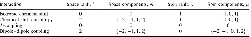
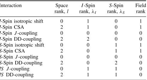
The symmetry-based approach to the design of rotor-synchronized pulse sequences exploits the rotational properties of the nuclear spin interactions. In general, each spin interac-tion may be expressed as a product of three terms, expressing the transformation properties of the interaction with respect to rotations of the molecular framework (‘space’), rotations of the nuclear spin polarizations (‘spin’) and rotations of the external magnetic field. These rotational properties may be summarized in terms of the threerotational rankswhich define each nuclear spin interaction. The set of rotational ranks forms the rota-tional signature of a nuclear spin interaction. The rotational signatures are summarized for the most important homonuclear interactions of spin-1/2 in Table 1.
As may be seen from Table 1, the significant nuclear spin interactions all have ranks 0, 1 or 2. For example, those interactions which are invariant to a particular type of rotation are assigned rank zero. Interactions which have the rotational symmetry of a p-orbital in atomic theory are assigned rank 1. Interactions which have the rotational symmetry of a d-orbital in atomic theory are assigned rank 2.
Consider, for example, the homonuclear dipolar interaction between nuclear spins. This has rank 2 with respect to both
Table 1 Rotational signatures of homonuclear spin interactions in diamagnetic systems of spin-1/2
Interaction Space rank,l Spin rank,λ Field rank
Isotropic chemical shift 0 1 1
Chemical shift anisotropy 2 1 1
J-coupling 0 0 0
spatial and spin rotations, indicating, for example, that a rotation of the molecular framework by 180◦ does not change the interaction strength, while a rotation through 90◦changes the sign of the interaction.
The chemical shift anisotropy interaction is more compli-cated, since it is a three-body interaction, involving the nuclear spins, the electronic environment and the external magnetic field. It has ranks 2, 1 and 1 with respect to molecular rota-tions, spin rotarota-tions, and external field rotarota-tions, respectively. This interaction changes sign if the nuclear spins are rotated by 180◦, with the molecules and the field held fixed. The CSA interaction also changes sign if the external field is rotated through 180◦, while the spin polarizations and the molecu-lar environment are held fixed. The CSA interaction does not change sign, on the other hand, if the molecules are rotated through 180◦, while the spins and the field are held fixed.
Many NMR textbooks conflate the ‘spin’ part and the ‘field’ part into one compound term, often called, confusingly, the ‘spin part’ of the interaction. This practice obscures the rotational properties and is best avoided.
There are also minor interactions such as the antisymmetric part of the chemical shift tensor (space, spin, field ranks of 1, 1 and 1), and theJ-coupling anisotropy (space, spin, field ranks of 2, 2 and 0), which are omitted here for simplicity.
The spherical ranks listed in Table 1 are defined as follows: An irreducible spherical tensor of rank l has 2l+1 compo-nents, with a component index m running from −l to +l in integer steps. A rotation interconverts these 2l+1 components according to the transformation equation:
R()TλmR()†=
+l
m=−l
TλmDmlm() (1)
Here R()are rotation operators and Dl
mm() is an
ele-ment of the(2l+1)-dimensional Wigner matrix. The symbol
indicates a triplet of Euler angles= {α, β, γ}defining a general three-dimensional rotation. Irreducible spherical ten-sors, Wigner matrices and Euler angles are discussed thor-oughly in the literature.4 A particularly useful compilation is given in Ref.53 The article Internal Spin Interactions & Rotations in Solids,Volume 4, summarizes many key results.
The Wigner elements have the following form:
Dmlm()=exp{−imα}d l
mm(β)exp{−imγ} (2)
wheredmlm(β)is called a reduced Wigner matrix element.
Although the detailed form of the Wigner matrices and the spherical tensors depends on the rank, and the approach appears to be mathematically complicated at first sight, the transformation properties are always the same, which permits a universal approach to pulse sequence theory.
2.2 Reference Frames
The discussion of spin interactions in rotating solids is facilitated by defining a set of reference frames (Figure 1).
2.2.1 The Principal Axis Frame P
The principal axis frame P provides the simplest form
of the spin interaction. For example, consider the through-space dipole – dipole interaction (DD interaction) between two
bRL
ΩMR
PΛ
ΩPMΛ
ωr
ΩRL zL
zR
L R
M
Figure 1 Definition of the reference frames in magic-angle spinning NMR experiments. (Adapted from Ref.82)
spins j and k. The z-axis of the principal axis frame Pj k
is oriented along the vector joining the spins j and k. In this frame, the spherical tensor components withm= ±1 and
m= ±2 vanish, leaving only the m=0 component. For the CSA interaction of spin j, the m= ±1 components vanish in the principal axis framePj, while them=0 andm= ±2
components remain finite.
In general, there are many different spin interactions, and each one has a different principal axis frameP.
2.2.2 The Molecular Frame M
The molecular reference frame M is fixed with respect to the molecular structure. It is usual to transform all of the different spin interactions into the common reference frame
M before further manipulations are imposed.
A principal axis frame P is related to the molecular
frame M by a set of three Euler angles, denoted
P M =
{α
P M, β
P M, γ
P M}. These Euler angles define the relative
orientation of the frames P and M. In general, there are
several spin interactions, each with a different set of Euler angles
P M, specifying its orientation with respect to the
common molecular frameM.
2.2.3 The Rotor Frame R
In a spinning solid, the orientation of the molecules with respect to the rotating sample holder (‘rotor’) is of great importance. The rotor-fixed frame R is defined such that its z-axis is along the rotational axis. The Euler angles
MR= {αMR, βMR, γMR}define the relative orientation of the
molecular reference frame and the rotor frame.
If the sample were a single crystal, with only one molecule in the asymmetric unit of the crystal structure, then all molecules in the sample would have the same set of Euler angles MR. In practice, the sample usually has an
orienta-tional distribution of some kind, and in the extreme case of a disordered sample such as a powder, the Euler anglesMRare
over all possible values of the Euler anglesMR. This is called
powder averaging.
The Euler angleγMR has special significance in the theory
of rotating solids. Molecules which have the same values of
αMR and βMR but different values of γMR are related by a
rotation around the rotor axis. This implies that the mechanical rotation of the sample causes such molecules to pass through the same cycle of laboratory frame orientations, but with a mutual time shift. This concept has been called acarousel,54 since the riders on a playground carousel follow the same circular path, but are shifted with respect to each other in time.
In some samples, it is convenient to include one or more reference frames intermediate between M and R. For example, in crystalline solids, it is common to define a crystal-fixed reference frame C, and a set of Euler angles MC=
{αMC, βMC, γMC} defining the orientations of the molecules
with respect to the crystal axes. If there is more than one more molecule in the crystal unit cell, then several sets of Euler anglesMC are needed. The orientation of the crystal
with respect to the rotor is defined through the Euler angles
CR. In ordered samples such as fibres, on the other hand, it
is useful to define a fibre director axis system D. The Euler angles MD relate the molecular axis system M to the fibre
director systemD, and a further set of Euler anglesDRrelate
the fibre director to the rotor axis. By factorizing the problem in this way, it is possible to define independent orientation distributions for the molecules with respect to the fibre, and for the fibres with respect to the rotor. An example of this approach is found in Refs.55,56If the sample is a powder, these intermediate axis systems are unnecessary, and they will be omitted in the following discussion.
2.2.4 The Laboratory Frame L
The laboratory frame is chosen so that its z-axis is along the external magnetic field. The relative orientation of the sample holder and the field are defined by the Euler angles
RL= {αRL, βRL, γRL}.
In magic-angle spinning NMR, the sample rotates at a fixed angular frequencyωrabout a fixed axis, subtending the magic
angleθmagic=arctan
√
2 with respect to the magnetic field. In these circumstances, the relevant Euler angles are given by
αRL=αRL0 −ωrt
βRL=θmagic=arctan
√ 2
γRL=arbitrary (3)
Here α0
RL defines the orientation of the rotor at time
pointt=0, which is rigorously defined as the start of signal acquisition (to be consistent with the normal definition of the Fourier transform, which involves an integral from t=0 to
t= ∞). If the rotation of the sample is not synchronized with the pulse sequence, the angleαRL0 varies randomly from transient to transient. If necessary, the rotation of the sample may be synchronized optically with the pulse sequence, so as to obtain reproducible and controllable values ofαRL0 . This is usually unnecessary in powder samples.
The negative sign in the expression for αRL is consistent
with the usual definition of the Euler angles53 and leads to
a right-handed rotation of the sample in the case that ωr is
positive.
The second Euler angleβRL is the angle between the rotor
axis and the field. For exact magic-angle spinning it is exactly equal to θmagic, but for other experiments, such as off-axis spinning, variable-axis spinning, or “zero-field in high-field” experiments, the angleβRL may take other values. In the rest
of this article, exact MAS is assumed.
In double rotation or dynamical angle spinning experi-ments,57 – 59 the time-dependence of the Euler angles
RL
is more complicated (see Double Rotation, Volume 3). I ignore such possibilities here (double rotation may be handled neatly by introducing an ‘outer rotor’ frame as an intermediate betweenRandL).
2.3 Frame Transformations
The following ‘chain rule’ for the Wigner matrices greatly facilitates the transformations of spin interactions between the different frames:
Dl(
AB)Dl(BC)=Dl(AC) (4)
For example, a given spin interactionmay be transformed from its principal axis frame into the laboratory frame using equation (1) and the following chain:
Dl(P M)D l
(MR)Dl(RL)=Dl(P L) (5)
Note the pattern of the subscripts. This notation greatly facilitates the task of concatenating multiple frame transfor-mations.
2.4 Rf Euler Angles
The mathematics of spherical tensor rotations may also be applied to the rotations of the nuclear spin polarizations by resonant rf fields. In general, a sequence of resonant rf fields induces a time-dependent rotation of the resonant spins, which may be expressed as follows:
Urf(t, t0)=exp{−iαrf(t)Iz}exp{−iβrf(t)Iy}exp{−iγrf(t)Iz} (6)
Here Urf is the propagator under the applied rf fields, starting from the initial point of the pulse sequence, denoted
t0, up to an arbitrary time t, and {I
x, Iy, Iz} are the total
angular momentum operators of the resonant spin species. In general, the propagator may be determined by integrating the Schr¨odinger equation:
d dtUrf(t, t
0)= −iHrf(t)U
rf(t, t0) (7)
under the boundary conditionUrf(t0, t0)=1. The operatorHrf is the spin Hamiltonian for the interaction with the rf field, and depends on the amplitude, phase and frequency of the applied rf field in the usual way.
trajectory from a given pulse sequence. Furthermore, it also possible to discover the pulse sequence that provides a desired trajectory of rf Euler angles.
2.5 Rotational Components
The mechanical rotation of the sample induces a time-dep-endent trajectory of the Euler anglesRL = {αRL, βRL, γRL},
while the rf pulse sequence induces a time-dependent trajectory of the Euler anglesrf= {αrf, βrf, γrf}. Suppose that a certain spin interaction has space rankl and spin rank λ. According to equation (1), the spatial rotation induces a mixing of the (2l+1) space components with m= −l,−l+1· · · +l. Similarly, in the interaction frame of the rf field (seeAverage Hamiltonian Theory,Volume 2), the spin rotations induce a mixing of the(2λ+1) spin components withµ= −λ,−λ+
1· · · +λ.
In the presence of sample rotation and resonant rf fields, each spin interactions may therefore be regarded as a super-position of(2l+1)×(2λ+1)components, characterized by quantum numbersmandµ:
H=
+l
m=−l
+λ
µ=−λ
H
lmλµ (8)
In the case of exact magic-angle spinning, the components withl=2 and m=0 vanish, due to the following property of the magic angle:
d002(θmagic)=0 (9)
Explicit expressions for the components H
lmλµ may be
found in Refs.45,60
A summary of the spin interaction components, in the case of exact magic-angle spinning, is given in Table 2.
2.6 Symmetry Classes
The space and spin trajectories may be synchronized so as to generate an average Hamiltonian containing desired combinations of quantum numbers {l, m, λ, µ} while other combinations are suppressed.
This is done by setting up periodic symmetry relationships between the mechanical and rf rotations. Consider two arbi-trary time points, separated by an interval nτr/N, where n
andN are integers, andτr = |2π/ωr|is the rotational period
of the sample. From equation (3), the continuous rotation of the sample imposes the following relationship on the spatial Euler angles:
αRL
t+nτr
N
=αRL(t)− 2π n
N βRL
t+nτr
N
=βRL(t) (10)
The rf pulse sequence imposes similar-looking rules on the rf Euler angles (equation (6)).
In the case of CNν
n sequences, the following Euler angle
symmetry is imposed:
βrf
t+nτr N
=βrf(t)
γrf
t+nτr N
=γrf(t)−
2π ν
N (11)
whereνis an integer, possibly different fromn. In the case of RNν
n sequences, the Euler angle symmetry
is slightly different:
βrf
t+nτr N
=βrf(t)±π
γrf
t+nτr N
=γrf(t)−
2π ν
N (12)
These symmetries apply to arbitrary time points within the pulse sequence.
The symbolCNν
n andRNnν is called thesymmetry class of
the rotor-synchronized pulse sequence. The integersN,nandν
are called thesymmetry numbersof the pulse sequence. As will be seen, the symmetry class defines a set ofselection rulesfor the average Hamiltonian, which may be used to manipulate the recoupling and decoupling properties of the pulse sequence.
2.7 Rotor-Synchronized Pulse Sequences
The symmetries in equations (11) and (12) only refer to two Euler angles; the behavior of the third Euler angleαrf is left completely free. This freedom implies that there are many inequivalent ways of implementing equations (11) and (12). Some simple possibilities are described below.
2.7.1 CNν
n Sequences
TheCNν
n Euler angle symmetries [equations (10) and (11)]
are generated by rotor-synchronized pulse schemes of the general form shown in Figure 2. The idea is thatnrotational periods of the sample are subdivided into N equal intervals. Each interval contains a radio frequency pulse sequence which is a cycle, i.e., it induces a rotation of the nuclear spins through an integer multiple of 360◦ (including zero). The radio-frequency phases of subsequent cycles are shifted with respect to each other by the angle 2π ν/N, causing a repeated incrementation (or decrementation) of the radio-frequency phase as one proceeds through the sequence. The integers n
[image:6.595.83.514.720.784.2]andν may therefore be interpreted as space and spinwinding numbers.39The sample rotates bodily throughnfull rotations, in the same time that it takes the radio-frequency phases to
Table 2 Components of homonuclear spin interactions in the interaction frame of an applied rf field, in the case of exact magic-angle spinning
Interaction Space rank,l Space components,m Spin rank,λ Spin components,µ
Isotropic chemical shift 0 0 1 {−1,0,1}
Chemical shift anisotropy 2 {−2,−1,1,2} 1 {−1,0,1}
J-coupling 0 0 0 0
0 1 2 3 N − 1
n complete sample revolutions
n complete phase revolutions Rf cycle
[image:7.595.58.267.92.567.2]Rf phase incrementation + 2pn/N
Figure 2 Construction ofCNν
n sequences
wrt
wrt
tr tr
2tr 2tr
3tr4tr
f f
0 0
t t t
t Spin
Spin Space
Space (a)
[image:7.595.69.262.359.574.2](b)
Figure 3 Visualization of the symmetry numbers for (a) C71 2
sequences, and (b)C1454 sequences. The left-hand helices represent the spatial rotation of the sample as a function of time. The right-hand helices depict the modulation of the rf phase as a function of time.n spatial rotations are completed in the same time asν spin rotations. The rf phase is modulated inN discrete steps, depicted by the planes in the right-hand diagrams. (Adapted from Ref.39)
advance throughν full rotations, inN equal steps. This idea is conveyed for the cases ofC71
2 andC1454 in Figure 3. These symmetry properties are independent of the internal structure of the rf cycles, providing that each cycle accom-plishes a final rotation through an integer multiple of 360◦.
For a proof that sequences with this structure generate the Euler angle symmetry given in equation (11), see Ref.60
For the sake of concreteness, consider a C712 sequence based upon the cyclic elementC=2700180180900, where ξφ
indicates a rectangular, resonant rf pulse with flip angleξ and
phase φ, and the angles are written in degrees. The full C712 sequence is as follows:
270018018090027051.43180231.439051.43270102.86180282.8690102.86−
270154.29180334.2990154.29270205.7118025.7190205.71−
270257.1418077.1490257.14270308.57180128.5790308.57 (13)
where the pulses are contiguous (no gaps in between). The rf field amplitude is chosen so that the entire sequence of 21 pulses fits exactly into two complete rotational periods of the sample. This requires that the spin nutation frequency in the rf field is exactly seven times the sample spinning frequency. The sequence in equation (13) is called POST-C7.37
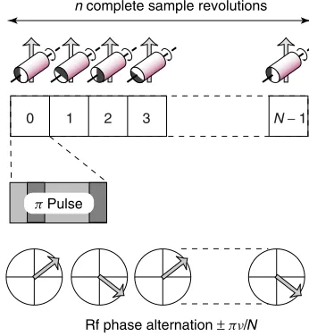
2.7.2 RNν
n Sequences
A construction scheme for generating sequences with the Euler angle symmetries in equations (10) and (12) involves the following steps:
1. Select a sequence of rf pulses which rotates the nuclear spins through 180◦ about thex-axis. Call this elementR. 2. Change the signs of all rf phases within the element R.
Call this phase-inverted elementR.
3. Select the rf amplitude so thatNelementsRoccupy exactly the same time interval asnrotational periods of the sample. The number of elementsNmust be even in the case ofRNν n
symmetry. 4. The RNν
n sequence consists of N/2 pairs of elements
RφR−φ, where φ is an overall phase shift, equal to φ =
π ν/N radians.
A simplified diagram of this procedure is shown in Figure 4 (step 2 above is omitted for simplicity). This looks similar to the set-up for a CNnν sequence, but with the two differences that each element provides a 180◦rotation, rather than a cycle, and that the rf phase is alternated between two values, rather than being incremented.
For a proof that sequences with this structure generate the Euler angle symmetry given in equation (12), see Ref.60
0 1 2 3 N − 1
n complete sample revolutions
Rf phase alternation ± pn/N
p Pulse
Figure 4 Construction ofRNν
[image:7.595.339.512.574.762.2]As a concrete example, suppose that one would like to build aR189
2sequence on the composite pulse 9009090900, which is known to have favorable homonuclear decoupling properties.61 The first step is to establish whether this element induces a 180◦rotation about thex-axis. This may be tested by rotating the three spin angular momentum operators, as follows:
Ix
900
−−−→Ix
9090
−−−→ −Iz
900
−−−→Iy
Iy
900
−−−→Iz
9090
−−−→Ix
900
−−−→Ix
Iz
900
−−−→ −Iy
9090
−−−→ −Iy
900
−−−→ −Iz (14)
From this it may be seen that the 9009090900sequence does transform Iz into −Iz, which is an appropriate property for
a 180◦ rotation about the x-axis, but that it also exchanges the operators Ix and Iy, which is not appropriate. A little
consideration leads to the conclusion that the 9009090900 sequence implements a rotation by 180◦ about an axis which is intermediate between thex-axis and the y-axis, i.e., phase shifted by 45◦. This may also be proved by rotation operator algebra.62
This defect may be remedied by phase shifting the whole sequence by−45◦. This leads to the element
R=90−45904590−45 (15)
which now implements the correct rotation. Changing the sign of all phases leads to
R=90
4590−459045 (16)
The desiredR189
2 sequence requires additional phase shifts ofφ = ±π×9/18 radians, or±90◦. The appropriate elements are therefore
Rφ=9045901359045 (17)
and
R
−φ=90−4590−13590−45 (18)
The fullR1892sequence has the following structure:
R189
2(version 1)= {904590135904590−4590−13590−45}9 (19)
where nine repetitions of the bracketed elements occupy exactly two rotational periods of the sample. If the phases are restricted to the interval 0 – 360◦, we get
R1892(version 1)= {9045901359045903159022590315}9 (20)
If the elementRcontains no internal phase shifts, or when it only contains 180◦ phase shifts, then the conversion of R intoRmay be ignored. For example, if a single 1800is used for the elementR, then theR189
2sequence is as follows:
R1892(version 2)= {18090180270}9 (21)
where nine repetitions of the bracketed elements occupy exactly two rotational periods of the sample.
Although the construction principles of theRNnν sequences appear to be quite complicated, the end result is sometimes very simple.
2.8 Effective Hamiltonian
In many circumstances, the behavior of the nuclear spins under a pulse sequence may be described using the theory described in Average Hamiltonian Theory,Volume 2. Sup-pose that the pulse sequence starts at time point t0 and lasts until time point t0+τ. Suppose also that the period of the pulse sequence is given byT =nτr, wherenis the space
wind-ing number. The propagator for the pulse sequence between the time pointst0andt0+τ is written as
U (t0+τ, t0)∼=Urf(t0+τ, t0)exp{−iH(t0)τ} (22)
whereUrfis the propagator for the rf field alone (equation (6)), H(t0)is theeffective Hamiltonian of the internal spin interac-tions, for a pulse sequence starting at pointt0.
In a rotating sample, the effective Hamiltonian depends upon the starting time point t0, since the orientation of the sample constantly changes.
The effective Hamiltonian may be approximated using the Magnus expansion:
H(t0)∼=H(1)(t0)+H(2)(t0)+ · · · (23)
where the first two terms are given by
H(1)
(t0)=T−1 t0+T
t0
dtHint(t)
H(2)
(t0)=(2iT )−1 t0+T
t0
dt2 t2
t0
dt1[Hint(t2),Hint(t1)] (24)
Here Hint is the internal spin Hamiltonian, expressed in the interaction frame of the rf field. This equation employs a consistent numbering system for the Magnus expansion terms, in which the kth Magnus term is proportional to a product of k Hamiltonians. Much literature uses a more awkward numbering, in which the indices start at zero.
The term H(1) is called the average Hamiltonian. The termH(2)is called thesecond-order correction to the average Hamiltonian, and so on.
If the internal spin Hamiltonian is small compared to the periodT of the pulse sequence, then the average Hamiltonian expansion may be terminated after the first or second term.
2.9 First-Order Selection Rules
The interaction frame spin Hamiltonian is a sum of many rotational components, as in equation (8). The average Hamil-tonian may therefore be written
H(1)
(t0)=
lmλµ
H(1)
lmλµ(t0) (25)
where
H(lmλµ1) (t0)=T−1
t0+T
t0
dtHlmλµ(t) (26)
Each of these components is modulated by the spatial rota-tion of the sample, and the rotarota-tions of the spin polarizarota-tions induced by the rf field. If the pulse sequence is a member of theCNnν orRNnν symmetry classes, then the synchronized modulations possess the symmetry properties summarized in equations (10) – (12).
In Refs.45,60it is shown that these symmetry properties lead toselection rules on the average Hamiltonian terms:
2.9.1 Selection Rules for CNν
n Sequences
ForCNnν sequences, the following selection rule applies:
H(1)
lmλµ=0 ifmn−µν=N Z (27)
whereZ is any integer, including zero.
2.9.2 Selection Rules for RNν
n Sequences
ForRNnν sequences, the following selection rule applies:
H(1)
lmλµ=0 ifmn−µν=
N
2Zλ (28) Here Zλ is any integer with the same parity as the spin
rankλ. Ifλis even, then Zλ takes the values 0,±2,±4, . . ..
Ifλis odd, thenZλtakes the values±1,±3,±5, . . ..
Equations (27) and (28) are the central results of symmetry-based pulse sequence theory. These two simple equations have wide consequences.
As a first example, consider a pulse sequence with sym-metry C71
2. Let us examine the fate of double-quantum dipole – dipole terms with quantum numbers {l, m, λ, µ} = {2,1,2,2}. Equation (27) states that the average Hamilto-nian of this term vanishes if the quantity mn−µν is not equal to an integer multiple of N. Substituting in the val-ues m=1, n=2, µ=2 and ν=1 we obtain mn−µν= (1×2)−(2×1)=0. This is an integer multiple ofN =7, so the term {l, m, λ, µ} = {2,1,2,2} is symmetry allowed. One cannot be sure whether this term actually exists without further calculation, but at least symmetry does not exclude it. Consider now the chemical shift anisotropy term with quantum numbers
{l, m, λ, µ} = {2,−2,1,1}. The expression mn−µν eval-uates to the value mn−µν=((−2)×2)−(1×1)= −5. This is not an integer multiple of 7, so this term issymmetry forbiddenin the first-order average Hamiltonian.
Now consider the fate of the same two terms under the symmetry R187
1, using the rule in equation (28). The homonuclear dipole – dipole terms have a spin rank λ=2,
which is even. Equation (28) implies that a dipole – dipole term is symmetry-forbidden unless mn−µν is equal to an even multiple of 9. For the term{l, m, λ, µ} = {2,1,2,2}, the expression mn−µν evaluates to (1×1)−(2×7)= −13. This is not an even multiple of 9, so the term {2,1,2,2} is forbidden under the symmetry R187
1. For the chemical shift anisotropy term{l, m, λ, µ} = {2,−2,1,1}, on the other hand, the expression mn−µν evaluates to the value mn−µν= ((−2)×1)−(1×7)= −9. This is an odd multiple of 9, and since the spin rank λ is also odd, this term is symmetry-allowed.
2.10 Space-Spin Selection Diagrams
The consequences of equations (27) and (28) are conve-niently evaluated using space-spin selection diagrams (SSS diagrams). Two examples are given in Figure 5 and 6.
The branching lines in these diagrams show the possible values ofmn−µν for the particular class of spin interaction, split up into the ‘space’ part mn and the ‘spin’ partµν. The number of branches depends on the type of spin interaction, according to Table 2, while the spacing between the branches depends on the symmetry numbers n and ν. The right-hand side of each diagram shows a barrier containing holes spaced by the symmetry number N. Those pathways that are
blocked by the barrier represent values of mn−µν which
do satisfy the inequalities in equations (27) and (28), and represent components that are symmetry-forbidden. Those pathways that pass through the holes in the barrier represent values of mn−µν which do not satisfy the inequalities in equations (27) and (28), indicating components that are symmetry-allowed. The SSS diagrams allow the consequences of the inequalities in equations (27) and (28) to be visualized clearly.
The positions of the holes depend on the symmetry class. For theCNν
n class of symmetries, the holes in the barrier occur
at levels 0,±N,±2N, . . .. For theRNν
n class of symmetries,
the positions of the holes depends on whether the spin rankλ
is even or odd. For even ranks, the holes occur at levels 0,±N,
±2N, . . ., as in the case ofCNnνsymmetries. For odd ranks, on the other hand, the holes occur at levels±N/2,±3N/2, . . ., whereN/2 is an integer, sinceN is even.
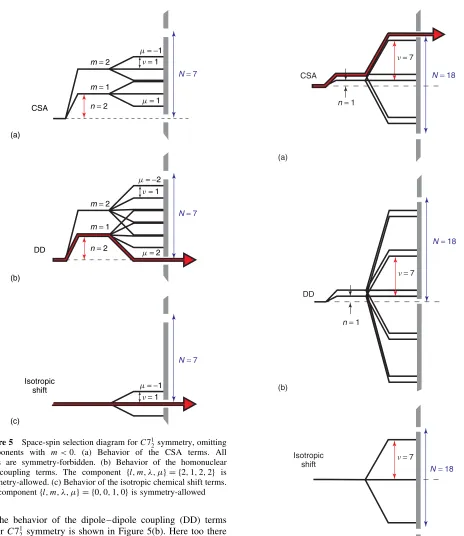
2.10.1 SSS Diagrams for C71
2 Symmetry
The behavior of the chemical shift anisotropy (CSA) terms under C71
DD CSA
(a)
(b)
(c)
Isotropic shift
m = 2
m = −1
m = −2
m = −1
n = 1
m = 1
m = 2
n = 1
n = 1 m = 1
N = 7
N = 7 N = 7
n = 2
m = 2
m = 1
[image:10.595.61.525.90.626.2]n = 2
Figure 5 Space-spin selection diagram forC71
2symmetry, omitting
components with m <0. (a) Behavior of the CSA terms. All terms are symmetry-forbidden. (b) Behavior of the homonuclear DD coupling terms. The component {l, m, λ, µ} = {2,1,2,2} is symmetry-allowed. (c) Behavior of the isotropic chemical shift terms. The component{l, m, λ, µ} = {0,0,1,0}is symmetry-allowed
The behavior of the dipole – dipole coupling (DD) terms underC71
2 symmetry is shown in Figure 5(b). Here too there are four branches in the space part, corresponding to the
m= {−2,−1,1,2}components in Table 2. Only the branches with non-negativem are shown, for the sake of clarity. Each of the space branches splits into five spin branches, with indices µ= {−2,−1,0,1,2}. As may be seen, the branch with {l, m, λ, µ} = {2,1,2,2} passes through a hole in the barrier, indicating that this component is symmetry-allowed. The mirror-image branch with{l, m, λ, µ} = {2,−1,2,−2}is also symmetry-allowed (not shown).
Since all the CSA terms are symmetry-forbidden, and the only symmetry-allowed DD terms have quantum numbers
µ= ±2, sequences with the symmetry C712 behave as CSA-compensated double-quantum recoupling sequences.
Now consider the SSS diagram for isotropic chemical shift
(a)
(b)
(c)
Isotropic shift
DD
N = 18
n = 7
CSA N = 18
n = 7
n = 1
N = 18 n = 7
[image:10.595.68.268.97.522.2]n = 1
Figure 6 Space-spin selection diagram forR1871symmetry, omitting components withm <0. (a) Behavior of the CSA terms. The compo-nent{l, m, λ, µ} = {2,2,1,−1}is symmetry-allowed. (b) Behavior of the homonuclear DD coupling terms. All components are symmetry-forbidden. (c) Behavior of the isotropic chemical shift terms. All components are symmetry-forbidden. Note that the positions of the holes change, depending on whether the spin rankλis odd or even
terms, shown in Figure 5(c). Since the space and spin ranks are
and three spin components, withµ= {−1,0,1}. The SSS dia-gram shows that the isotropic shift component{l, m, λ, µ} = {0,0,1,0} is symmetry-allowed under C712 symmetry. This implies thatC71
2 sequences are vulnerable to isotropic chem-ical shifts, unless additional precautions are taken. We return to this issue later.
2.10.2 SSS Diagrams for R187
1 Symmetry
The behavior of the CSA terms underR1871 symmetry is shown in Figure 6(a). The left-hand side shows the two space branches withm=1 and 2. The m=0 component vanishes in the case of exact magic-angle spinning. The space branches are spaced vertically by 1 unit, according to the winding numbern=1. Each branch splits into three spin components, with indicesµ= {−1,0,1}, and spaced vertically by 7 units, according to the winding numberν=7. Since the spin rankλ
of the CSA terms is equal to 1, which is an odd number, the barrier on the right contains holes at odd multiples ofN/2, which is equal to 9 in this case. The holes in the barrier are therefore at levels ±9,±27, . . .. As may be seen, the CSA term{l, m, λ, µ} = {2,2,1,−1}passes through a hole, which indicates thatR1871 symmetry is aCSA recoupling sequence.
The behavior of the DD terms under R187
1 symmetry is shown in Figure 6(b). The space branches with m=1 and 2 split into five spin components, with indices µ= {−2,−1,0,1,2}. In the case of DD couplings, the spin rank
λ is equal to 2, which is an even number. As a result, the barrier on the right contains holes at even multiples of 9, i.e., 0,±18,±36, . . .. As may be seen, the barrier blocks all of the DD terms. This indicates that sequences withR187
1symmetry are insensitive to homonuclear dipole – dipole couplings, to first order.
The behavior of the isotropic chemical shift terms under
R1871 symmetry is shown in Figure 6(c). None of the three components withm=0 and µ= {−1,0,1} pass through the barrier. This indicates that sequences withR187
1symmetry are insensitive to isotropic chemical shifts, to first order.
One may conclude thatR187
1 sequences accomplish recou-pling of the CSA interactions, compensated to first order for homonuclear DD couplings and isotropic chemical shifts.
2.11 Higher-Order Selection Rules
In many cases, the first-order Magnus term (the average Hamiltonian) is not a sufficiently good approximation to the effective Hamiltonian of a pulse sequence. Although the higher-order correction terms H(2),H(3), . . . are more complicated than the first-order terms, they are also subject to selection rules in the case of pulse sequence symmetry.
By analogy with equation (25), the second-order term H(2) may be written as a superposition of many rotational components:
H(2)
(t0)=
l2m2λ2µ2
l1m1λ1µ1 H(2)
l2m2λ2µ2,l1m1λ1µ1(t
0) (29)
where each component is given by
H(2)
l2m2λ2µ2,l1m1λ1µ1(t 0)
=(2iT )−1 t0+T
t0
dt2 t2
t0
dt1[Hl2m2λ2µ2(t2),Hl1m1λ1µ1(t1)] (30)
The horrifying complexity is moderated by the following selection rules:
ForCNν
n sequences, the following selection rule applies:
H(2)
l2m2λ2µ2,l1m1λ1µ1=0 if
m2n−µ2ν=N Z
AND
m1n−µ1ν=N Z
AND
(m2+m1)n−(µ2+µ1)ν=N Z
(31)
whereZis any integer, including zero. ForRNν
n sequences, the following selection rule applies:
H(2)
l2m2λ2µ2,l1m1λ1µ1=0 if
m2n−µ2ν=
N 2Zλ2
AND m1n−µ1ν=
N 2Zλ1
AND
(m2+m1)n−(µ2+µ1)ν=
N 2Zλ2+λ1
(32)
whereZλ2 is an integer with the same parity asλ2,Zλ1 is an
integer with the same parity as λ1, and Zλ2+λ1 is an integer
with the same parity asλ2+λ1.
These selection rules are proved in Refs.45,60
Although the second-order selection rules do not usually allow the elimination of all undesirable terms, they do greatly reduce the labor required to evaluate the terms. For example, in general, there are 208 components to theH(2)term involving commutators of dipole – dipole coupling and CSA interactions. In the presence of a R146
2 sequence, only 16 of these are symmetry-allowed.
The R-sequence selection rule equation (32) is more restric-tive than that for C-sequences equation (31). As a result, R-sequences tend to have smaller numbers of higher-order terms than C-sequences, which often translates into improved per-formance.
The second-order selection rules allow a straightforward count of the number of symmetry-allowed terms of a particular type. Higher-order term counts may be used to get a feel for the qualitative performance of a particular symmetry, without performing detailed calculations.41,45 However, this rather crude criterion should not be relied on completely.
It is possible to extend these second-order selection rules to arbitrarily high orders.45
2.12 Scaling Factors
The selection rules provide information on which terms are symmetry-forbidden. However, they provide no information on the magnitude of the symmetry-allowed terms.
In general, the form of a symmetry-allowed first-order term is as follows:
H
lmλµ(t0)=κlmλµ[Alm] Rexp{−i
m(αRL0 −ωrt0)}Tλµ (33)
where [Alm
]Ris a component of the spatial tensor of interaction
, expressed in the rotor-fixed frame R, and T
λµ is a
component of the spin tensor of interaction , expressed in the laboratory frame. The factor κlmλµ is called the scaling
The scaling factor may be a complex number. Its magnitude is always less than one, which indicates that the suppression of unwanted terms is always accompanied by a reduction in the magnitude of the symmetry-allowed terms.
2.12.1 Scaling Factor Formulae
General formulae for the scaling factors are given in Ref.60 In the case of CNnν sequences, the scaling factor for a symmetry-allowed term{l, m, λ, µ}is given by
κlmλµ=
τ−1dml0(βRL)
τ
0
dt dµλ0(−βrf(t))exp{i(µγrf(t)+mωrt)} (34)
whereτ =nτr/N is the duration of a basic elementC,τr =
|2π/ωr| is a rotor period, and βrf(t ) and γrf(t ) are rf Euler angles [equation (6)]. The basic element C is assumed to extend from timet =0 to t=τ.
In the case ofRNν
n sequences, the scaling factor is given
by
κlmλµ=τ−1dml0(βRL) ×τ
0
dt dµλ0(−βrf(t))exp{i(µγrf(t)−µ
π ν
N +mωrt)}(35) There is an extra complex factor in this case, since the first element of aRNν
n sequence is not the same as the basic
element.
The scaling factor is calculated most readily if the basic elements of the pulse sequence do not contain any rf phase shifts, or if the phase shifts are integer multiples of 180◦. This is the case of amplitude-modulated basic elements. For example,C=2700180180900 is an amplitude-modulated basic element, while R=90−45904590−45 is a phase-modulated basic element. In the case of amplitude-modulated basic elements, the rf Euler angles are given by
βrf(t)= t
0
dtωnut(t)
γrf(t)=π/2 (36)
where ωnut is the amplitude of the rf field, expressed as a nutation frequency (180◦ phase shifts may be taken into account by reversing the sign ofωnut).
The calculation of the scaling factor is more difficult if the basic element is phase modulated. General formulae are given in Ref.60Andreas Brinkmann has written aMathematica63 pro-gram which provides the scaling factors of general sequences of rectangular pulses. The program is available on the web (http://www.soton.ac.uk/∼mhl).
2.12.2 Physical Interpretation
The formulae for the scaling factor, equations (34) and (35) contain three factors. The first term,dl
m0(βRL)is purely spatial,
and concerns the transformation of spatial rank-ltensors by the physical rotation of the sample. This term depends on the tilt of the rotation axis with respect to the magnetic field. The second term dλ
µ0(−βrf(t )) corresponds to the time-dependent transformation of rank-λ spin operators by the rf field. The
third term (the complex exponential factor) takes into account the physical rotation of the sample within the duration of each pulse sequence element. The formula for the R-sequence scaling factor, equation (35), contains a further phase factor, which arises because the first element of a R-sequence is phase shifted with respect to the basic elementR.
In general, it is desirable that the magnitude ofκlmλµis as
large as possible. It helps if one develops a physical feel of howκlmλµ is generated.
In most cases, the angle βRL is equal to the magic angle,
so that the first term dl
m0(βRL) is not open to manipulation
(an exception is provided by the ‘zero-field in high-field’ pulse sequences, where the choice of the spinning angle is an important element of the pulse sequence design).
In many cases, the symmetry number N is much larger thann. In this case, the duration of each element is much less than a rotor period, and it is possible to ignore the rotation of the sample during the individual rf elements, as a first approximation. This corresponds to the neglect of the mωrt
terms in equations (34) and (35). This is called the quasi-static approximation.
In the quasi-static limit, only the rf rotations affect the accumulating time average ofTλµspin operators. For example,
consider the problem of double-quantum recoupling. The relevant Wigner element in this case is d2
20(βrf), which is proportional to sin2(βrf). This term is always positive, and is maximized at βrf=90◦ andβrf=270◦. It follows that the main contributions to the scaling factor are obtained when the Euler angleβrfis close to the values 90◦or 270◦. At the same time, the Euler angle γrf should be kept fixed. As shown in equation (36), this may be ensured by using an amplitude-modulated basic element.
The simplest cyclic element is C=3600. The rotation under this pulse takes the Euler angle βrf linearly from 0 to 360◦. Double-quantum excitation is accomplished near the ‘hot spots’ at βrf=90◦ and βrf=270◦. No double-quantum excitation is achieved, on the other hand, at the ‘cold spots’ βrf=0 and βrf=180◦. The element C=3600 spends equal time near the ‘hot’ and ‘cold’ spots. Nevertheless, the appropriate Wigner element is always positive, so the scaling factor is satisfactory (|κ2122| =0.157 for the case of
C71
2symmetry).
The scaling factor may be improved by turning the rf field off near the ‘hot spots’ βrf=90◦ and βrf=270◦, allowing the double-quantum operators more time to accumulate. An example of this technique is given by the sequence
C=900−τω−1800−τω−900 (37)
where the ‘window’ durationτωis selected so that the overall
element occupies an interval τ =nτr/N. In the limit of
infinitely strong and short pulses, the element in equation (37) provides a greatly improved scaling factor of |κ2122| =0.308 for the case ofC71
2symmetry. Although the scaling factor may be increased by introducing windows, this method has not been used very often, perhaps because the strong rf pulses make the problem of proton decoupling more acute (see below).
scheme.36In this case, each of the double-quantum ‘hot spots’ at βrf=90◦ and βrf=270◦ are traversed twice during each element. The scaling factor of |κ2122| =0.155 is almost the same as for the simple elementC=3600, which has|κ2122| = 0.157. The values are slightly different because of the rotation of the sample during the rf element.
In the quasi-static limit, the efficiency of double-quantum recoupling is greatly reduced if the Euler angleγrfis allowed to vary. For example, the scaling factor for the phase-modulated element C=3600360120360240 is given by |κ2122| =0.047 in the case ofC71
2symmetry.
If the values of N and nare comparable, the quasi-static approximation breaks down. In this case, it is necessary to think much more carefully about how the physical rotation of the sample and the spin rotations combine. Amplitude-modulated elements are no longer optimal as far as the scaling factor is concerned. For example, consider the symmetryC715, which provides similar selection rules to C712 (except that the {l, m, λ, µ} = {2,±1,2,∓2} terms are selected, rather than {2,±1,2,±2}). In the case of C715 symmetry, the scaling factor for the allowed term{l, m, λ, µ} = {2,1,2,−2} is given by |κ212−2| =0.064 for the amplitude-modulated standard element C=3600360180. This low scaling factor is due to the considerable rotation of the sample during the C element, leading to a strong variation of the ωrt term in
equation (34).39,40The scaling factor may be greatly improved by using the phase-modulated elementC=3600360120360240. For the case ofC715symmetry, one obtains the value|κ212−2| = 0.144.39 The improvement in scaling factor arises because the modulations of the Euler angle γrf due to the rf phase shifts compensate the modulation of theωrt term, to a good
approximation. Note that the phase shifts must be performed in the correct sense: The scaling factor for the element C=3600360240360120, in the case of C71
5 symmetry, is only
|κ212−2| =0.044.
In some cases, pulse sequences work even if the scaling factor is very small. For example, the most commonly-used version of the RFDR pulse sequence33,34 employs XY phase cycling and conforms toR41
4symmetry. This symmetry is appropriate for zero-quantum DD recoupling, since it allows the homonuclear DD terms{l, m, λ, µ} = {2,±1,2,0} and {2,±2,2,0}, while suppressing other DD terms and all chemical shift terms. However, the first reports of this pulse sequence used anRelement consisting of a strong 180◦pulse followed by a ‘window’ in which the rf field is turned off. This is a puzzling choice of basic element, since the scaling factors for all symmetry-allowed DD terms vanish if the rf pulses are infinitely short. In fact, this pulse sequence reasonably well because the rf pulses always have a finite duration, so that the scaling factor is small but finite. In addition,J-couplings and higher-order effects play a role. Recent implementations of RFDR take a more sophisticated approach.64,65
2.12.3 Vanishing Scaling Factors
In many cases, the scaling factors for some symmetry-allowed terms are deliberately set to zero. For example, the symmetry C71
2 allows the isotropic chemical shift term
{l, m, λ, µ} = {0,0,1,0}. Pulse sequences with this symmetry are therefore vulnerable to isotropic shift variations. The basic elementsC=3600, 3600360180and 9003601802700set the scal-ing factor κ0010 to zero, compensating these pulse sequences
for isotropic chemical shifts or resonance offset effects. R -symmetries such as R146
2 do not need this precaution, since all isotropic chemical shift terms are symmetry-forbidden in this case.
Another example is provided by the MELODRAMA sequence for homonuclear dipolar recoupling.66Some versions of this sequence are based onC41
1 symmetry. In these cases, the isotropic shift term{l, m, λ, µ} = {0,0,1,0}is symmetry-allowed, but may be suppressed by using basic elements of the form C=(360k)0, where k is an integer. Other versions of the MELODRAMA sequence66haveR411symmetry, which suppresses all isotropic shift terms without extra precautions. None of these symmetries, however, remove all of the CSA terms.
The recently-described C-REDOR sequences67are remark-able examples of how the basic element may be designed so as to destroy undesirable symmetry-allowed terms. The main variants of C-REDOR sequences are based upon C31 3 and C71
7 symmetry. These symmetries allow CSA terms of the form {l, m, λ, µ} = {2,±2,1,0} and {2,±1,1,0}, the isotropic shift term {0,0,1,0}, and also the homonuclear DD coupling terms {2,±2,2,0} and {2,±1,2,0}. However, by choosing a basic elementC=9003601802700, the scaling fac-tors of all terms vanish, except for those belonging to the CSA terms{2,±1,1,0}. These sequences may therefore be used to selectively recouple CSA terms while suppressing the isotropic chemical shifts and homonuclear DD couplings. C-REDOR has been applied to the selective recoupling of heteronuclear DD interactions,67 which behave in the same way as the CSA terms, if the rf field is resonant with only one spin species (see below).
The vanishing scaling factors of certain terms under specific pulse sequences is probably due to additional symmetries. This is a promising area for further theory.
2.13 Orientation Dependence
In most cases, the magnitudes of the recoupled spin inter-actions depend on the orientation of the molecular reference frame with respect to the rotor. The only exceptions are when isotropic spin interactions such as theJ-coupling or the isotropic chemical shift are selected, or in the special case of ‘zero-field in high-field’ experiments.28,29
The orientation-dependence of the recoupled spin interac-tions creates both problems and opportunities. A powerful feature of the symmetry theory is that it allows the form of the orientation-dependence to be manipulated qualitatively by choosing certain combinations of symmetry numbers.
The recoupled spin Hamiltonian in equation (33) is propor-tional to the spatial tensor component in the rotor-fixed frame, defined through the transformation chain
[Alm] R=
m,m [Alm]
P
Dmlm( P M)D
l
mm(MR) (38)
Here [A
lm]P are components of the spatial tensor,
expressed in its own principal axis frame. The expression in equation (38) depends on the three Euler angles MR =
{αMR, βMR, γMR} defining the orientation of the molecular