Manuscript received September 16, 2015. This work was supported in part by the Ministry of Science and Technology, Taiwan, R.O.C., under Contract No. MOST 104-2221-E-159-005.
Chih-Ming Hsu is with the Ming-Hsin University of Science and Technology, Hsin-Fong, Hsinchu 320401, Taiwan (phone:
0
0 ( )
) ( )
,
(X W w X w W X w
f m T
i i
i
(1)where wi is the weight; W is the weight vector; i(X) is
the feature; (X) is the feature vector; w0is the bias.
Furthermore, Vapnik [16] designed a general error function, called the ε-insensitive loss function, to evaluate the prediction error, as follows
otherwise | ) , ( | | ) , ( | if 0 )) , ( , (
d f X W
W X f d W X f d L (2) Therefore, we can express the penalty (loss) by
Q i w X W d i T
i ( ) 0 , 1,..., (3)
Q i
d w X
W i i
T ( ) ', 1,...,
0
(4)
Q i
i0, 1,...,
(5)
Q i
i 0, 1,...,
'
(6)
where i and i' are non-negative slack variables which are
used to measure the errors above and below the predicted function, respectively, for each data point. Therefore, the empirical risk minimization problem can be defined as [16,
17]
Q i i Q i i C W 1 ' 1 2 || || 21
(7)
subject to the constraints in (3)–(6), where C is a user specified parameter for the trade-off between complexity and losses. To solve the optimization in (7), the Lagrangian in primal variables are constructed as follows
Q i i i i i i i T i Q i i i i i T Q i i Q i i Q i i T P w X W d d w X W C W W w W L 1 ' ' ' 0 1 ' 0 1 1 ' 1 ' ' 0 ) ( ) ( ) ( 2 1 ) , , , ,' , , , ( (8)where T
Q)
,..., (1
and T
Q)
,...,
( ' '
1 '
are slack
variable vectors; T
Q)
,..., (1
, T
Q) ,..., ( ' ' 1 ' , T Q) ,..., (1
and T
Q)
,...,
( ' '
1 '
are the Lagrangian
multiplier vectors for (3)–(6), respectively. The partial derivatives of LPwith respective to the primal variables have
to vanish at the saddle point for optimality. Therefore,
) ( ) ( 0 ) ' , ,' , ,' , , , ( 1 ' 0 i Q
i i i
P W X
W w W
L
(9) 0 ) ( 0 ) ' , ,' , ,' , , , ( 1 ' 00
Q i i i P w w WL
(10)
i i
i
PW w C
L
0 ) ' , ,' , ,' , , ,
( 0 (11)
' '
'
0, , ,' , ,' , ') 0
, (
i i
i
PW w C
L (12)
Substitute (9), (11) and (12) into (8), the simplified dual form LD then can be obtained, as follows
Maximize
Q i Q j j i j j i i Q i i i i i Q i i D X X K d L 1 1 ' ' 1 ' ' 1 ) , ( ) )( ( 2 1 ) ( ) ( ) ' , ( (13)
Q i i i 1') 0
( (14)
Q i
C
i , 1,...,
0 (15)
Q i
C
i , 1,...,
0' (16)
where K(Xi,Xj)(Xi)(Xj) is called the kernel function. Furthermore, the data points for which i or 'i is
not zero are called the support vectors. The optimal weight vectors can then be obtained with the Lagrangian optimization done as follows
) ( ) ˆ ˆ ( ) ( ) ˆ ˆ ( ˆ 1 ' 1 ' k n k k k i Q i i
i X X
W
s
(17)
where ns is the number of support vectors, and the index k
only runs over support vectors. In addition, the optimal bias can be obtained, by exploiting the Karush–Kuhn–Tucker (KKT) conditions [18, 19] as follows
nus s
i n k i i k k i us X X K d n w 1 1
0 ( , ) sign( )
1
ˆ (18)
where nus is the number of unbounded support vectors with
Lagrangian multipliers which satisfy 0iC , and
'
ˆ ˆ
i i i
. Thus, we can obtained the approximated regression model as follows
Q i i i i ii K X X w
X
f( ,ˆ,ˆ') (ˆ ˆ') ( , ) ˆ0. (19)
B.Genetic Algorithms
Genetic algorithms (GAs) are robust adaptive optimization techniques which can perform an efficient probabilistic search in a high dimensional space[20] based on the natural and biological evolution. For applying GAs to a specific problem, two issues including (1) encoding a potential solution, and (2) identifying the fitness function (objective function) must be defined in advance. The encoding a potential solution is a genetic representation of a solution which is a vector composed of several components (genes), called a chromosome. The initial population of chromosomes is usually generated according to some principles or randomly selected. The qualities of potential solutions are then evaluated through the fitness function (objective function). In addition, the optimization is achieved through the selection and matching (crossover). Besides the matching, small mutations can also occur in the new offspring. The bad solutions are then replaced with new ones based on some fixed strategies and the chromosomes evolve through successive iterations, called generations. The solution procedure continues until the stopping criteria are satisfied. Let P(g) and C(g) represent the parents and offspring in the current generation g, respectively. The general procedure of GAs can be described as follows [21]:
g←0;
initialize P(g); evaluate P(g);
while (not termination condition) do
recombine P(g) to yield C(g); evaluate C(g);
select P(g+1) from P(g) and C(g); g←g+1;
end end
III. PROPOSED HYBRID FORECASTING APPROACH
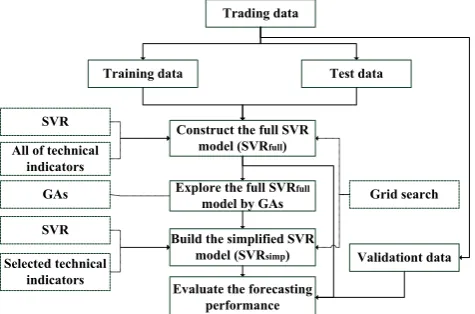
In this study, a hybrid approach that applies the support vector regression (SVR) and genetic algorithms (GAs) was proposed to forecast the stock prices. The proposed procedure comprises three stages. At the first stage, the collected data are used to calculate the technical indicators. The technical indicators along with closing stock price in the first or the second or the third trading day in the future for each trading day are divided into two groups: (1) training data and (2) test data, according to the odd or even number of the trading datum. The SVR is then utilized to construct a full forecasting model, call SVRfull, for the first or the second or
the third trading day in the future or the third trading day in the future based on the training and test data. Notably, the optimization of parameters C, and in the SVR are done with the grid-search approach [22]. Furthermore, the 10-fold cross validation is applied to determine the best SVR model by minimizing the MSE. In the second stage, the genetic algorithms (GAs) screen out the technical indicators which are critical to the stock prices by exploring the well-constructed SVRfull model and the fitness function in
GAs is the total MSE regarding the training and test data. Finally, the SVR technique is applied again to construct the simplified model, called SVRsimp, to be the final forecasting
model based on the selected technical indicators chosen from the second stage and the data for constructing the SVR simplified model include the training and test data divided in the first stage. The forecasting performance is evaluated by the MSE, MAPE and R-square. The proposed approach is conceptually illustrated in Fig. 1.
IV. CASE STUDY
A.Collect trading data and calculate technical indicators
In this study, the daily trading data including the open piece, highest price, lowest price and closing price of the TAIEX, are collected during 1/1/2009 to 12/13/2014 form the CMoney database (www.cmoney.com.tw). The technical indicators are then calculated based on these trading data. Sixteen technical indicators are involved in this study according to previous study in [23–29].
B.Build the full SVR forecasting models
The data where the input variables (predictors) are the technical indicators calculated previously and the output variable (response) is the closing stock price in the next trading day in the TAIEX from 1/1/2009 to 12/31/2011 are divided into two groups including the (1) training data and (2) test data according to the odd or even number of the trading datum. The SVR technique is then utilized to construct the full forecasting model, call SVRfull_1. Similarly, the full
forecasting models where the output variables (responses) are the closing stock prices in the next 2 trading days and next 3 trading days, i.e. the second trading day and the third trading day in the future, respectively, can then be built, call SVRfull_2 and SVRfull_3, respectively. The information about
[image:3.595.48.286.568.725.2]the obtained SVR full forecasting models are summarized in Table 1. From Table 1, we can conclude that the MSEs are small and the R-squares are good enough (all R-squares are larger than 0.98). Therefore, we are confident that we can use these SVR full forecasting models for further exploring the critical technical indicators by GAs.
C.Explore the full SVR models
The full SVR forecasting models listed in Table 1 are further explored by GAs. The crossover and mutation rates are set as 0.5 and 0.1, respectively, and the population size is set as 40 according to our past experience. Furthermore, the maximum searching cycles (generations) are set as 400 and the GAs stop searching the better solution until the fitness function does not improve during the last 20 generations. The fitness function in this study is evaluated by:
Total GAs
MSE MSE
fitness . (20)
where MSEGAs is the total of training and test MSEs of the
SVR when forecasting the stock prices based on the selected
Trading data
Test data Training data
Validationt data Construct the full SVR
model (SVRfull) SVR
All of technical indicators
Explore the full SVRfull
model by GAs
Build the simplified SVR
model (SVRsimp)
GAs
SVR
Selected technical indicators
Evaluate the forecasting performance
Grid search
Fig. 1. The proposed hybrid forecasting approach.
TABLEI
THE INFORMATION ABOUT THE OBTAINED SVRFULL FORECASTING
MODELS.
Types of forecasting 1 day’s
forecasting
2 days’ forecasting
3 days’ forecasting Total number of the
training data
374 374 374
Total number of the test data
374 374 373
Training MSE 0.000400008 0.000668459 0.000990816
Test MSE 0.000332013 0.000712591 0.000914454
Training R2 0.99132 0.984839 0.997627
Test R2 0.99247 0.983897 0.979025
technical indicators chosen by GAs and MSETotalis the MSE
regarding the training and test data by using the full SVR forecasting model built in the previous section to forecast the stock prices. In addition, the GAs are implemented for five times for each full forecasting models. The acquired results are shown in Table 2. Notably, the boldface represented the best results selected for each full SVR model by maximizing the fitness and the model’s name indicates the simplified SVR forecasting model built according to the selected technical indicators. From Table 2, we can conclude that the GAs can effectively select the technical indicators which are critical to the closing stock prices. Therefore, the values of fitness are all very high and they can exceed one in the most cases. In some cases, the values of fitness in the selected results of GAs are smaller than one, but are very close to one. In other words, the GAs can sift the important technical indicators which are significant to the closing stock prices in the future from the all technical indicators without significantly reducing the forecasting performance. In
addition, the CPU time is less than 6 minutes thus the GAs method can be considered efficient. Based on these observations, we can conclude that the GAs really can determine the important technical indicators to the closing stock prices, thus constructing the simpler and more accurate forecasting models by removing the useless (unimportant) noisy technical indicators effectively and efficiently.
D. Evaluate the forecasting performance
The forecasting performance of the full and simplified forecasting SVR models through MSE, MAPE and R-square when they applying to the unknown validation data, i.e. the trading data from 1/1/2012 to 12/31/2014. The results are given in Table 3. Table 3 shows that all of the simplified SVR models are better than the full SVR models constructed by the single SVR technique based on the MSE or MAPE or R-square. Hence, we can conclude that the proposed approach in this study can improve the forecasting performance of SVR models by screening out the critical technical indicators by GAs for all of the cases in forecasting the closing stock prices in the next day, next 2 days and next 3 days. Thus, the proposed method in this study can be considered effectively. Furthermore, we can find that the forecasting performance can improve better by implementing
the proposed approach in this study while comparing to the
single SVR technique if the forecasting time is farer. In other words, the GAs can improve the forecasting performance more significantly when the forecasting time is farer. This is very helpful to the investors. From the above discussions, we have confidence that the proposed method in his study is an effective and efficient tool and can be used in the real investment situation for investors.
V.CONCLUSIONS
This study proposes the hybrid approach based on the SVR and GAs. The proposed method can screen out the critical technical indicators for forecasting the stock prices thus avoiding the noisy technical indicators and improving the forecasting performance. The proposed procedure is demonstrated by a case study aiming at forecasting the closing stock price of the TAIEX stock markets for the first, the second and the third trading day in the future. The experimental results indicate that the GAs can effectively determine the technical indicators which are critical to the closing stock prices by exploring the full SVR models. In addition, the GAs can sift the important technical indicators which are significant to the closing stock prices in the future from the all technical indicators without significantly reducing the forecasting performance. Furthermore, the CPU time is less than 6 minutes. Hence, the GAs method can be considered efficient. Next, the GAs can improve the forecasting performance more significantly when the forecasting horizon is longer. Therefore, we can conclude that the GAs really can choose the important technical indicators to the closing stock prices, thus constructing the simpler and more accurate forecasting models by removing the useless (unimportant) noisy technical indicators effectively and efficiently.
ACKNOWLEDGMENT
The author would like to thank the Ministry of Science and Technology, Taiwan, R.O.C., for its support of this research under Contract No. MOST 104-2221-E-159-005.
REFERENCES
[1] M.-J. Kim, S.-H. Min and I. Han, “An Evolutionary Approach to the
Combination of Multiple Classifiers to Predict a Stock Price Index,”
Expert Systems with Applications, vol. 31, no. 2, pp. 241–247, 2006.
[2] H.-Y. Lee, “A Combination Model of Multiple Artificial Intelligence
Techniques Based on Genetic Algorithms for the Prediction of Korean
TABLEII
THE INFORMATION ABOUT THE EXECUTION RESULTS OF GAS.
Types of forecasting 1 day’s
forecasting
2 days’ forecasting
3 days’ forecasting Implementation #1
(cycle #, fitness, CPU time (seconds))
(35,1.01354209, 186.37)
(32,1.00425825, 189.93)
(42,0.99554228, 267.83) Implementation #2
(cycle #, fitness, CPU time (seconds))
(25,1.01517491, 132.17)
(31,1.00436390, 173.68)
(34,0.99972333, 214.23)
Implementation #3 (cycle #, fitness, CPU
time (seconds))
(32,1.00933667, 169.89)
(40,1.00415327, 221.27)
(31,0.99556640, 193.89) Implementation #4
(cycle #, fitness, CPU time (seconds))
(22,1.01487199, 118.12)
(23,1.00113771, 133.36)
(35,0.99875523, 218.67) Implementation #5
(cycle #, fitness, CPU time (seconds))
(29,1.01584577, 155.42)
(34,1.00433296, 182.91)
(38,0.99662135, 225.39) The total number of
selected technical 11 12 14
TABLEIII
THE EVALUATION OF FORECASTING PERFORMANCE
Types of forecasting 1 day’s
forecasting
2 days’ forecasting
3 days’ forecasting
Full models’
names SVRfull_1 SVRfull_2 SVRfull_3
MSE 0.000188 0.001416 0.001875 MAPE 0.006866 0.016074 0.018626 R2 0.988803 0.922638 0.895563
Simplified models’
names SVRsimp_1 SVRsimp_2 SVRsimp_3 MSE 0.000181 0.000587 0.001032 MAPE 0.006763 0.010636 0.014304
Stock Price Index (KOSPI),” Enture Journal of Information Technology, vol. 7, no. 2, pp. 33–43, 2008.
[3] S.-H. Hsu, J. J. P. A. Hsieh, T.-C. Chih and K.-C. Hsu, “A Two-Stage
Architecture for Stock Price Forecasting by Integrating
Self-Organizing Map and Support Vector Regression, Expert Systems
with Applications, vol.36, no.4, pp. 7947–7951, 2009.
[4] W.-T. Pan, “Performing Stock Price Prediction Use of Hybrid Model,”
Chinese Management Studies, vol. 4, no. 1, pp. 77–86, 2010.
[5] 42. C.-Y. Yeh, C.-W. Huang and S.-J. Lee, “Multiple-Kernel Support
Vector Regression Approach for Stock Market Price Forecasting,”
Expert Systems with Applications, vol. 38, no. 3, pp. 2177–2186, 2011.
[6] Y. Zuo and E. Kita, “Stock Price Forecast Using Bayesian Network,”
Expert Systems with Applications, vol. 39, no. 8, pp. 6729–6737, 2012.
[7] C.-M. Hsu, “A Hybrid Procedure with Feature Selection for Resolving
Stock/Futures Price Forecasting Problems,” Neural Computing and
Applications, vol. 3, no. 4, pp. 651–671, 2013.
[8] T. Xiong, Y.-K. Bao and Z.-Y. Hu, “Multiple-Output Support Vector
Regression with a Firefly Algorithm for Interval-Valued Stock Price
Index Forecasting,” Knowledge-Based Systems, vol. 55, pp. 87–100,
2014.
[9] C. Wu, P. Luo, Y.-L. Li, L. Wang and K. Chen, “Stock Price
Forecasting: Hybrid Model of Artificial Intelligent Methods,”
Inzinerine Ekonomika-Engineering Economics, vol. 26, no.1, pp. 40–48, 2015.
[10] B. Boser, I. Guyon I. and V. Vapnik, “A Training Algorithm for
Optimal Margin Classifiers,” in Proceedings of the 5th Annual ACM
Workshop on Computational Learning Theory, Pittsburgh, PA, 1992, pp. 144–152.
[11] I. Guyon, B. Boser and V. Vapnik, “Automatic Capacity Tuning of
Very Large VC-Dimension Classifiers,” in Advances in Neural
Information Processing System, vol. 5, S.-J. Hanson, J. D. Cowan and C. L. Giles, Eds. San Mateo, CA: Morgan Kaufmann, 1993, pp. 147–155.
[12] C. Cortes and V. Vapnik, “Support-Vector Networks,” Machine
Learning, vol. 20, no. 3, pp. 273–297, 1995.
[13] B. Schölkopf, C. Burges and V. Vapnik, “Extracting Support Data for a
Given Task,” in Proceedings of First International Conference on
Knowledge Discovery and Data Mining, Menlo Park, CA, 1995, pp. 252–257.
[14] V. Vapnik, S. Golowich and A. Smola A, “Support Vector Method for
Function Approximation, Regression Estimation, and Signal
Processing, in Advances in Neural Information Processing Systems,
vol. 9, M. C. Mozer, M. I. Jordan and T. Petschel, Eds. Cambridge, MA: MIT Press, 1997, pp. 281–287.
[15] H. Drucker, C. J. C. Burges, L. Kaufman L, A. Smola and V. Vapnik,
“Support Vector Regression Machines,” in Advances in Neural
Information Processing Systems, vol. 9, M. C. Mozer, M. I. Jordan and T. Petsche, Eds. Cambridge, MA: MIT Press, 1997, pp. 155–161.
[16] V. Vapnik, Statistical Learning Theory. New York: Wiley, 1998.
[17] V. Vapnik, The Nature of Statistical Learning Theory. New York
Springer-Verlag, 1995.
[18] W. Karush, “Minima of Functions of Several Variables with
Inequalities as Side Constraints , Master Thesis, University of Chicago, Chicago, IL, 1939).
[19] H. Kuhn and A. Tucker, “Nonlinear Programming,” in Proceedings of
the 2nd Berkeley Symposium on Mathematical Statistics and Probabilistics, Berkeley, CA: University of California Press, 1951, pp. 481–492.
[20] D. E. Goldberg, Genetic Algorithm in Search, Optimization and
Machine Learning. New York: Adison-Wesley, 1989.
[21] M. Gen and R. Cheng, Genetic Algorithms and Engineering
Optimization, New York: John Wiley & Sons, 2000.
[22] C.-C. Chang and C.-J. Lin, “LIBSVM: A Library for Support Vector
Machines,” ACM Transactions on Intelligent Systems and Technology,
vol. 2, no. 3, pp. 2:27:1–27:27, 2013.
[23] K.-J. Kim and I. Han, “Genetic Algorithms Approach to Feature
Discretization in Artificial Neural Networks for the Prediction of Stock
Price Index,” Expert Systems with Applications, vol. 19, no. 2, pp.
125–132, 2000.
[24] K.-J. Kim and W. B. Lee, “Stock Market Prediction Using Artificial
Neural Networks with Optimal Feature Transformation,” Neural
Computing and Applications, vol. 13, no. 3, pp. 255–260, 2004.
[25] P. M. Tsang, P. Kwok, S. O. Choy, R. Kwan, S. C. Ng, J. Mak, J. Tsang,
K. Koong and T.-L. Wong, “Design and Implementation of NN5 for Hong Kong Stock Price Forecasting,” Engineering Applications of Artificial Intelligence, vol. 20, no. 4, pp. 453–461, 2007.
[26] P.-C. Chang and C.-H. Liu, “A TSK Type Fuzzy Rule Based System
for Stock Price Prediction,” Expert Systems with Applications, vol. 34,
no. 1, pp. 135–144, 2008.
[27] H. Ince and T. B. Trafalis, “Short Term Forecasting with Support
Vector Machines and Application to Stock Price Prediction,”
International Journal of General Systems, vol. 37, no. 6, pp. 677–687, 2008.
[28] C.-L. Huang and C.-Y. Tsai, “A Hybrid SOFM-SVR with a
Filter-Based Feature Selection for Stock Market Forecasting,” Expert
Systems with Applications, vol. 36, no. 2, pp. 1529–1539, 2009.
[29] R. K. Lai, C.-Y. Fan, W.-H. Huang and P.-C. Chang, “Evolving and
Clustering Fuzzy Decision Tree for Financial Time Series Data
Forecasting,” Expert Systems with Applications, vol. 36, no. 2, pp.