Intelligent Water Drops (IWD) Algorithm for
COCOMO II and COQUAMO Optimization
Abdulelah G. Saif, Safia Abbas, and Zaki Fayed,
Member, IAENG
Abstract—Software effort, time and quality estimation is an
important aspect in software projects. Accurate estimates are required for efficiently developing software systems. Many estimation methods have been proposed during the last 30 years. Among those methods, COCOMO II , the most widely used model due to its simplicity for estimating the effort in person-month and the time in months for a software project at different stages, and COQUAMO, the model used to estimate the quality of the software project in defects/KSLOC (or some other unit of size). Nowadays, estimation models are based on neural network, the fuzzy logic modeling etc. for finding the accurate estimation for software development effort, time and quality. Because there is no clear guideline for designing neural networks and also fuzzy logic approach is hard to use. A meta-heuristic, Intelligent Water Drops (IWD) algorithm, can offer some improvements in accuracy for software effort, time and quality estimation. This work introduces an optimized cost-quality model by adapting the IWD algorithm for optimizing the current coefficients of COCOMO II model to achieve more accurate estimation of software development effort and time. The next work applies the same thing for COQUAMO. The experiment has been conducted on NASA 93 software projects.
Index Terms—COCOMOII, IWDalgorithm, Softwarecost andquality estimation
I. INTRODUCTION
A successful software project must be completed on time, within budget, and deliver a quality product that satisfies users and meets requirements. Unfortunately, many software projects fail. A report by the Standish Group noted that only a third of all software development projects were successful, in terms of they met budget, schedule, and quality targets [1]. Software projects usually don’t fail during the implementation and most project fails are related to the planning and estimation steps. During the last decade several studies have been done in term of finding the reason of the software projects failure. Galorath et al. performed an intensive search between 2100 internet sites and found 5000 reasons for the software project failures. Among the found reasons, insufficient requirements engineering, poor planning the project, suddenly decisions at the early stages of the project and inaccurate estimations were the most important reasons [2]. So accurate software cost, time and quality estimation is necessary and is critical to both
Manuscript submitted July 10, 2015; revised July 23, 2015. The authors
gratefully acknowledge the support of Ain Shams University and Yemen government in supporting them.
Abdulelah Ghaleb Farhan Saif is Ph.D student at Ain Shams University, Egypt (phone: 00201154415035; [email protected]). Safia Abbas Mahmoed Abbas is lecturer at Ain Shams University, Egypt ( [email protected]).
Zaki Taha Ahmed Fayed is Emeritus Professor at Ain Shams University, Egypt ( [email protected]).
developers and customers. Software cost estimation is related to how long and how many people are required to complete a software project. Software cost estimation starts at the proposal state and continues throughout the life time of a project [3].The major part of cost of software development is the human-effort and most cost estimation methods focus on this aspect and give estimates in terms of person-month [4]. In spite of accurate planning, well documentation and proper process control during software development, occurrences of certain defects are inevitable. These software defects may lead to degradation of the quality which might be the underlying cause of failure [18]. Therefore, in order to manage budget, schedule and quality of software projects, various software estimation methods have been developed. Among those methods, COCOMO II is the most widely used model due to its simplicity for estimating the effort in person-month and the time in months for a software project at different stages, and COQUAMO is the model used to estimate the quality of the software project in terms of defects/KSLOC (or some other unit of size). Today's models are based on neural network, genetic algorithm, the fuzzy logic modeling etc [4]. In this paper, the meta-heuristic, Intelligent Water Drops (IWD), is adapted for optimizing the current coefficients of COCOMO II model that estimates the effort and time required for developing the software project.
The rest of the paper is organized as follows: in section II architecture of the proposed model, section III COCOMO model, section IV related work, section V dataset description, section VI IWD algorithm, section VII assumption and representation, section VIII the proposed IWD algorithm, section IX results analysis and section X discusses and concludes the paper
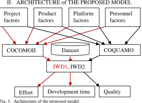
[image:1.595.306.553.580.760.2]II. ARCHITECTURE of THE PROPOSED MODEL
Fig. 1. Architecture of the proposed model.
This model combine COCOMO II model with COQUAMO Dataset
IWD1, IWD2
Effort Quality
Project factors
Product factors
Platform factors
Personnel factors
COCOMOII
Development time
COQUAMO model to estimate cost, time and quality and allows making tradeoff between cost, time and quality, if needed.
The arrows with red color show the work which is done in this paper; IWD1 optimizes COCOMO II coefficients, whereas IWD2 optimizes COQUAMO coefficients which will be done in the next work.
III. COCOMO MODEL
Constructive Cost Model (COCOMO) is one of the best-known and best-documented software effort and time estimation methods [4]. It was proposed by Boehm in 1981 and it has the following hierarchy-
1. Model 1 (Basic COCOMO Model):- The basic
COCOMO model computes software development effort and cost as a function of program size expressed in estimated lines of code (LOC).
2. Model 2 (Intermediate COCOMO Model):-
Intermediate COCOMO model computes software development effort as a function of program size and set of 15 cost drivers that include subjective assessment of the products, hardware, personnel and project attributes.
3. Model 3 (Detailed COCOMO Model):- The detailed
COCOMO model incorporates all characteristics of the intermediate version with an assessment of the cost driver‘s impact on each step (analysis, design, etc) of the software engineering process [3].
The underlying software lifecycle is the waterfall lifecycle. It has been experiencing difficulties in estimating the cost of software developed to new life cycle processes and capabilities including rapid-development process model, reuse-driven approaches and object-oriented approaches. For these reasons the newest version COCOMO ІІ was developed.
4. COCOMO II model:- The capabilities of COCOMO II
are size measurement in KLOC, Function Points, or Object Points. COCOMO II adjusts for software reuse and reengineering. This new model served as a framework for an extensive current data collection and analysis effort to further refine and calibrate the model's estimation capabilities. This model has three sub-models defined below [4]:
(i) Application Composition Model: involves
prototyping efforts to resolve potential high-risk issues like user interfaces, software/system interaction, performance, or technology maturity. It uses object points for sizing.
(ii) Early Design Model: involves exploration of alternative software/system architectures. It involves use of function points for sizing and a small number of additional cost drivers.
(iii) Post-Architecture (PA) Model: involves actual development and maintenance of a software product. It uses source instructions and/or function points for sizing, with modifiers for reuse and software breakage. Unfortunately not all of the extensions of COCOMO II are already calibrated and therefore still they are experimental. Only Post Architecture model is implemented in a calibrated software tool. COCOMO II describes 17 Effort Multipliers (EMs) that are used in
the Post-Architecture model. For more information about COCOMO II see [4] and [17].
COCOMO II post architecture method calculates the software development effort (in person months) by using the following equation:
Effort = A × (SIZE)E ×
17
1 i
EMi. (1)
A- multiplicative constant with value 2.94 that scales the effort according to specific project conditions. Size - Estimated size of a project in Kilo Source Lines of Code or Unadjusted Function Points. E - An exponential factor that accounts for the relative economies or diseconomies of scale encountered as a software project increases its size. EMi - Effort Multipliers. The coefficient E is determined by weighing the predefined scale factors (SFi) and summing them using following equation:
E = B + 0.01×
5
1 i
SFi (2)
The development time (TDEV) is derived from the effort according to the following equation:
TDEV = C × (Effort)F (3)
Latest calibration of the method shows that the multiplier C is equal to 3.67 and the coefficient F is determined is a similar way as the scale exponent by using following equation:
F = D + 0.002 ×
5
1 i
SFi (4)
B=0.91,D=0.28.
When all the factors and multipliers are taken with their nominal values, then the equations for effort and schedule are given as follows:
Effort = 2.94 × (Size)1.1 [9] (5)
Duration: TDEV = 3.67 × (Effort)3.18 (6)
COCOMO II is clear and effective calibration process by combining Delphi technique with algorithmic cost estimation techniques. It is tool supportive and objective. This model is repeatable, versatile. But its limitation is that most of extensions are still experimental and not fully calibrated till now [4]. The values of effort multipliers and scale factors used in the implementation are taken from [4].
IV. RELATED WORK
Lately many researchers have been focused on cost estimation field for the software projects using the AI techniques. But it is not possible to say that AI is 100% percent to estimate the costs accurately, however the studies showed that the AI techniques have been more efficient in comparison to the algorithmic techniques. COCOMO is a model for cost and time estimation of the software projects among the algorithmic methods [14].
lowest in terms of effort estimation accuracy. The COCOMO II follows a pessimistic approach, while the approach followed by the other three is optimistic. The results with regard to duration estimation, SEER-SEM had the lowest MMRE value, whereas all four methods are pessimistic in estimating duration. COCOMO II performed better in estimating the project duration than the effort. SEER-SEM was (relatively) successful in both effort and duration estimation. TruePlanning performed better in estimating effort than duration. The major limitation for their study is the partial project information in the ISBSG project repository. This study suggests that these models need improvements regarding prediction accuracy.
In [2], authors discuss popular software cost estimation techniques including expert-judgment, analogy-based, function points, COCOMO II, neural networks and fussy logic and also in [9] authors discuss, in addition to previous methods in [2], PSO and GP in terms of their capabilities, strengths and weaknesses in order to project manager choose the best estimation method according to the information and data available about project to avoid project failures.
In [3], authors present the strength and weakness of various software cost estimation methods which include algorithmic methods such as function points, COCOMO 81, COCOMO II, SLIM ,SEL, Doty, Walston-Felix, Bailey-Basil and Halstead models and non-algorithmic methods such as expert-judgment, analogy-based, Top-Down, Bottom-up, Parkinson’s Law and Price-to-win and perform a comparative analysis using COCOMO dataset among algorithmic models and the performance is analyzed and compared in terms of MMRE (Mean Magnitude of Relative Error) and PRED (Prediction). They also focus on some of the relevant reasons that cause inaccurate estimation. At the end, authors conclude that all estimation methods are specific for some specific type of projects. It is very difficult to decide which method is better than all other methods because every method or model has an own significance or
importance. To understand their advantages and
disadvantages is very important when we want to estimate our projects.
One of the problems with using COCOMO today is that it does not match the development environment of recent times, so authors, in [10] and [11], presented a detailed study on the use of binary genetic algorithm as an optimization algorithm which provided solution to adjust the uncertain and vague properties of software effort drivers by tuning Constructive Cost Model (COCOMO) parameters in order to get better effort estimate. The performance of the developed models, in [10] and [11], was tested on NASA software project dataset and the developed model in [10] compared to the pre-existed model. The developed model in [10] was able to provide better estimation capabilities.
As today's project evaluation based on old coefficients of COCOMO II Post Architecture (PA) model may not match the required accuracy, authors in [4], use the concept of genetic algorithm to optimize the COCOMO II PA model coefficients to achieve accurate software effort estimation and reduce the uncertainty of COCOMO II post architecture model coefficients i.e. A, B, C and D. Experiments have been conducted on Turkish and Industry dataset and the
results are compared between original COCOMO II PA and optimized COCOMO II PA . Optimized COCOMO II PA was better.
In [12], author proposed a new model by combining 15 cost drivers of intermediate COCOMO model with Walston-Felix model to get optimum effort value and in [13], authors modified intermediate COCOMO model by introducing some more parameters to predict the software development effort more precisely using GA for PROMISE project dataset.
In [14], authors have proposed a hybrid model based on GA and ACO for optimization of the effective factors’ weight in NASA dataset software projects. The results of the experiments show that the proposed model is more efficient than COCOMO model in software projects cost estimation and holds less Magnitude of Relative Error (MRE) in comparison to COCOMO model.
In [15], authors have investigate the role of fuzzy logic technique in improving the effort estimation accuracy using COCOMO II by characterizing inputs parameters using Gaussian, Trapezoidal and Triangular membership functions and comparing their results. NASA (93) dataset is used in the evaluation of the proposed Fuzzy Logic COCOMO II. After analyzing the results, it had been found that effort estimation using Gaussian member function yields better results for maximum criterions when compared with the other methods.
V. DATASET DESCRIPTION
Experiments have been conducted on NASA 93 data set found in [5] to optimize effort and time. The dataset consist of 93 completed projects with its size in kilo line of code (KLOC) and actual effort in person-month and development time in months. Effort multipliers and scale factors rating from Very Low to Extra High are also given in this dataset.
VI. INTELLIGENT WATER DROPS (IWD)
ALGORITHM
IWD is swarm-based optimization algorithm which has been inspired from natural rivers that find optimal/nearly optimal paths to their destination. IWD finds optimal/ nearly optimal solutions for optimization problems, by simulating the mechanisms that happen in the natural river system and implementing them in the form of algorithm [6]. It depends on both static and dynamic parameters, such as, iteration number, water drops number, number of nodes, initial soil, initial velocity, soil updating parameters, velocity updating parameters, local and global soil updating parameters, soil of edge, visited node list and IWD velocity. IWD represents the problem in the form of a graph G = (V, E), with the set of nodes V, and the set of edges E [6, 7].
VII. ASSUMPTION and REPRESENTATION
IWD is first invented for combinatorial optimization problems, and there is only one paper [16] modifies it to be used for continues optimization problems with binary coding of edges. In order to use IWD for continues optimization problems such as optimizing the COCOMO II Post Architecture model and maintaining the original structure of IWD, the coefficients of COCOMO II PA
soil soil soil soil soil soil soil soil
..
l
..
..
...
model, A, B, C and D, are assumed to be represented by the following graph via adding virtual nodes numbered from 0 to 9 and connecting those nodes to each coefficient as in figure 2.
Each of the four coefficients is expressed by 4 digits which are chosen among 10 digits by IWD algorithm according to minimum probabilities; First digit is integral part of a coefficient and the remaining 3 are fractions part.
The soils are placed on the virtual edges between coefficients and digits as in figure 2.
[image:4.595.45.308.176.265.2]
Fig. 2. Coefficients representation.
VIII. THE PROPOSED IWD ALGORITHM:
To optimize the COCOMO II PA model coefficients, The main steps of proposed IWD algorithm are in figure 3.
IX. RESULT ANALYSIS
IWD parameters initial values: Number of IWDs=5,
Initial Soil=10000 , velocity=100, local and global soil
updating parameters=0.9, av = 1,bv = 0.01, cv = 1,as = 1,bs
= 0.01 and cs = 1.
The best result is achieved using 10000 iterations and a solution set is received from which the best solution is chosen i.e. a solution with the best fitness function values
(FitnessEffort, FitnessTime). The final best solution
obtained for coefficients is: 3 7 6 2 | 1 0 0 5 | 4 4 8 4 | 0 2 8 8 According to this solution, the resulting optimized COCOMO II PA model coefficients are the following: A=3.762, B=1.005, C=4.484 and D=0.288. Current COCOMO II PA model coefficients are the following: A=2.94; B=0.91; C=3.67; D=0.28.
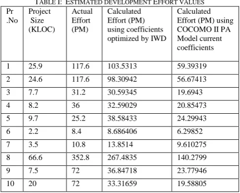
Tables, table I and table II, show the comparison among the actual, effort and time, values and estimated, effort (person month) and time (months), values for the first ten project dataset using IWD algorithm optimized and current COCOMO II PA model coefficients with their estimated project size.
1. Set parameters and determine dataset
2. Initialize the soils of virtual edges between coefficients
and their digits.
3. While (termination condition not met) do
4. IWDs are placed on the first node i.e. coefficient A and move to the next until it reaches node D.
5. IWDs choose 4 digits among 10 digits as values for
coefficients according to minimum probabilities and add the digits to their visited lists. If there is no improvement in one of the fitness functions
(FitnessEffort) in step 10, IWDs choose 4 digits for
each coefficient randomly.
6. IWDs update their velocity.
7. IWDs update soils on edges between coefficients and
chosen digits and load some soils according to IWD algorithm equation 4 in [6].
8. Calculate estimated development effort and time for
each project j in the dataset using the values of coefficients chosen by IWDs.
9. Each IWD i calculates Magnitude of Relative Error
(MRE) for each project j, the equations used for
[image:4.595.48.292.589.785.2]effort and time, respectively are:
FitnessEij=|ActualEj– EstimatedEij | / ActualEj (7)
FitnessTij=|ActualTj– EstimatedTij | / ActualTj (8).
i - the IWD number,
j – the project number,
ActualEj – the actual software project effort,
EstimatedEij - the estimated software project effort
using IWD i,
ActualTj - the actual software project time and
EstimatedTij - the estimated software project time.
10. The fitness functions ( Mean Magnitude of Relative
Error MMRE) for effort and time are calculated as
the average value of all projects specific fitness values calculated during steps 8 and 9 which depends on the difference between real and estimated effort and time. So, the fitness functions values should be minimized.
FitnessEffort= 1/n *
n
j 1
FitnessEij (9)
FitnessTime = 1/n *
n
j 1
FitnessTij (10)
11. Find the iteration best solution.
12. Update the soils of virtual edges that form current
best solution according to IWD equation 6 in [6].
13. End while.
14. Return the values of coefficients and the estimated
effort and time.
Fig. 3. Proposed IWD algorithm.
The graphical comparison among effort values and among time values described in table I and table II, respectively is shown in figure 4 and figure 5, respectively.
A B C D
9
0
0
9
0
9
0
9
TABLE I: ESTIMATED DEVELOPMENT EFFORT VALUES
Pr .No
Project Size (KLOC)
Actual Effort (PM)
Calculated Effort (PM) using coefficients optimized by IWD
Calculated Effort (PM) using COCOMO II PA Model current coefficients
Comparison among actual, optimizd and COCOMO II model effort values vs estimated project size in KLOC
0 50 100 150 200 250 300 350 400
25.9 24.6 7.7 8.2 9.7 2.2 3.5 66.6 7.5 20
Progect Size (KLOC)
E
ff
ort
(
P
M
) Actual Effort Optimized Effort(IWD) COCOMO II Model Effort
Fig. 4. Comparison among Effort values vs. Size.
Comparison among actual, optimizd and COCOMO II model time values vs estimated project size in KLOC
0 5 10 15 20 25
25.9 24.6 7.7 8.2 9.7 2.2 3.5 66.6 7.5 20
Progect Size (KLOC)
Ti
m
e
(
M
on
ths
)
Actual Time Optimized Time(IWD) COCOMO II Model Time
Fig. 5. Comparison among Time values vs. Size.
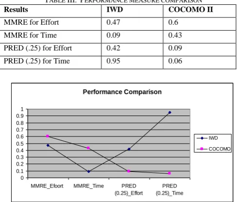
Table III and figure 6 compare the MMRE (Mean
Magnitude of Relative Error) and PRED (.25) which show
the performance of IWD and COCOMO II in estimating the effort and time for the whole dataset.
MMRE=
n
1
*
n
j 1 j
j j
Actual
|
Estimated
-Actual
|
(11)
MREj =
Actualj
|
Estimatedj
-Actualj
|
(12)
PRED (p) = k / n (13) k is the number of projects where MRE is less than or equal to p, and n is the total number of projects.
Performance Comparison
0 0.1 0.2 0.3 0.4 0.5 0.6 0.7 0.8 0.9 1
MMRE_Efoort MMRE_Time PRED (0.25)_Effort
PRED (0.25)_Time
IWD COCOMO I I
Fig. 6. Performance measure comparison.
From table III and figure 6, the MMRE of IWD for effort
and time is lower than that of COCOMO II and PRED(0.25)
of IWD for effort and time is larger than that of COCOMO II.
It shows clearly that optimized coefficients by IWD algorithm produces more accurate results than the old coefficients. So, IWD algorithm can offer some significant improvements in accuracy and has the potential to be a valid additional tool for the software effort and time estimation.
X. DISCUSSION and CONCLUSION
This paper adapts IWD algorithm for optimizing COCOMO II coefficients. The proposed algorithm is tested on NASA 93 dataset and the obtained results are compared with the ones obtained using the current COCOMO II PA model coefficients. The proposed model is able to provide good estimation capabilities. It is concluded that
By having the appropriate statistical data describing the software development projects, IWD based coefficients can be used to produces better results in comparison with the results obtained using the current COCOMO II PA model coefficients.
The results show that, in the sample projects taken from the dataset, the results obtained using the coefficients optimized with the proposed algorithm are better than the ones obtained using the current coefficients.
The results also shows that in the sample projects
taken from the dataset, the results obtained using the coefficients optimized with the proposed algorithm are close to the real effort and time values.
The results also shows that in the whole dataset, the
MMRE of IWD is less than that of COCOMO II and
PRED(0.25) is larger than that of COCOMO II.
In the future work or the next paper, we adapt IWD algorithm for optimizing the coefficients of COQUAMO model to complete the implementation of the proposed model.
TABLE II: ESTIMATED DEVELOPMENT TIME VALUES
Pr. No
Project Size (KLOC)
Actual Time (Months)
Calculated Time (Months) Using coefficients Optimized by IWD
Calculated Time (Months) using
COCOMO II PA model current coefficients
1 25.9 15.3 17.06107 10.5749 2 24.6 15 16.80866 10.43705 3 7.7 10.1 12.00955 7.76328 4 8.2 10.4 12.23024 7.888731 5 9.7 11 12.83961 8.233734 6 2.2 6.6 8.357022 5.641787 7 3.5 7.8 9.559073 6.350325 8 66.6 21 22.42472 13.45205 9 7.5 13.6 12.67039 8.184016 10 20 14.4 12.30812 7.75153
TABLE III: PERFORMANCE MEASURE COMPARISON
Results IWD COCOMO II MMRE for Effort 0.47 0.6
MMRE for Time 0.09 0.43
PRED (.25) for Effort 0.42 0.09 PRED (.25) for Time 0.95 0.06
[image:5.595.49.289.51.544.2] [image:5.595.306.550.67.275.2]REFERENCES
[1] Gary B. Shelly, Harry J. Rosenblatt, “Systems Analysis and Design Ninth Edition”, Shelly Cashman Series®, 2012.
[2] Vahid Khatibi, Dayang N. A. Jawawi, “Software Cost Estimation Methods: A Review ”, Volume 2 No. 1, Journal of Emerging Trends in Computing and Information Sciences, 2011.
[3] Sweta Kumari , Shashank Pushkar, “Performance Analysis of the Software Cost Estimation Methods: A Review ”, International Journal of Advanced Research in Computer Science and Software Engineering, Volume 3, Issue 7, July 2013.
[4] Astha Dhiman, Chander Diwaker, “Optimization of COCOMO II Effort Estimation using Genetic Algorithm”, American International Journal of Research in Science, Technology, Engineering & Mathematics, 2013.
[5] Nasa 93 dataset contains effort and defect information available at
http://promisedata.googlecode.com/svn/trunk/effort/nasa93-dem/nasa93-dem.arff.
[6] Hamed Shah-Hosseini, “The intelligent water drops algorithm: a nature-inspired swarm-based optimization algorithm”, Int. J. Bio-Inspired Computation, Vol. 1, Nos. 1/2, 2009.
[7] Priti Aggarwal, Jaspreet Kaur Sidhu, Harish Kundra, “applications of intelligent water drops” , IISRO, Multi-Conference, Bangkok, 2013.
[8] Derya Toka, Oktay Turetken, “Accuracy of Contemporary Parametric Software Estimation Models: A Comparative Analysis”, 2013 39th Euromicro Conference Series on Software Engineering and Advanced Applications.
[9] K.Ramesh and P.Karunanidhi, “Literature Survey on Algorithmic and Non- Algorithmic Models for Software Development Effort Estimation”, International Journal of Engineering and Computer Science ISSN: 2319-7242, Volume 2, Issue 3, March 2013, Page No. 623-632.
[10] Brajesh Kumar Singh, A. K. Misra, “ Software Effort Estimation by Genetic Algorithm Tuned Parameters of Modified Constructive Cost Model for NASA Software Projects”, International Journal of Computer Applications (0975 – 8887), Volume 59– No.9, December 2012.
[11] Alaa F. Sheta, “Estimation of the COCOMO Model Parameters Using Genetic Algorithms for NASA Software Projects”, Journal of Computer Science 2 (2): 118-123, 2006.
[12] Kavita Choudhary, “GA Based Optimization of Software Development Effort Estimation”, IJCST Vol. 1, Issue 1, September 2010.
[13] Chandra Shekhar, Yadav, Raghuraj Singh, “Tuning of COCOMO II Model Parameters for Estimating Software Development Effort using GA for PROMISE Project Data Set”, International Journal of Computer Applications (0975 – 8887) Volume 90 – No 1, March 2014.
[14] Isa Maleki, Ali Ghaffari, and Mohammad Masdari, “A New Approach for Software Cost Estimation with Hybrid Genetic Algorithm and Ant Colony Optimization”, International Journal of Innovation and Applied Studies ISSN 2028-9324 Vol. 5 No. 1 Jan. 2014, pp. 72-81.
[15] Ashita Malik, Varun Pandey, Anupama Kaushik, “An Analysis of Fuzzy Approaches for COCOMO II”, I.J. Intelligent Systems and Applications, 2013, 05, 68-75 Published Online April 2013 in MECS (http://www.mecs-press.org/).
[16] Hamed Shah-Hosseini, “An approach to continuous optimization by the Intelligent Water Drops algorithm, 4th International Conference of Cognitive Science (ICCS 2011).
[17] “COCOMO II Model definition manual, version 2.1”, 1995 – 2000 Center for Software Engineering, USC.