Abstract— The scope of application of linear optimization techniques in decision problems is expanded by using some existing and some newly described modeling techniques for logical phenomena. The current practice is to model Boolean logic relations such that the values of these expressions are constrained to be TRUE. There are situations though in decision making, where the statuses of the logical relations need to be resolved within the context of the solution, rather than being pre-assigned. The techniques specified here show how this requirement can be met with logical expressions that can assume either TRUE or FALSE values. It is now possible to specify all possibilities and consequences due to the value of the logical expression, as part of the problem itself. It thus enables modeling of nested If-Then-Else conditions as declarative programs. The relevance of these techniques is demonstrated on a scheduling problem.
Index Terms— Logic, Mixed-integer linear programming (MILP), Optimization, Production Scheduling
I. INTRODUCTION
n many of the linear optimization problems involving continuous and discrete variables, a subset of the governing constraints may have logical expressions to describe specific structural or operational requirements or situations. The formulation of the optimization problem for these problems is facilitated through logical constructs which have either a TRUE or FALSE status. In some problems the relevant expression models a pre-assigned status like TRUE or FALSE. For example, Logical OR is TRUE. In some other cases there is a need though to depict a conditional choice based on the outcome of a previous decision or occurrence of an event. In these cases a subset of logical expressions could carry either a TRUE or FALSE value which cannot be assigned apriori but has to be decided as part of the optimal solution search. In the above example, depending on the TRUE or FALSE state of the logical OR, consequent decisions may differ. In certain temporal decision making problems like scheduling, the status of a decision at a certain time step needs to be carried forward in time to avoid the choice of a subsequent decision which is incompatible with the earlier decision. In evolving solutions of such optimization problems one needs different
Manuscript received January 08, 2016 for review.
Dhananjay Karandikar is working at Tata Consultancy Services, Pune, Maharashtra, India. email: [email protected].
K.P.Madhavan is Professor Emeritus, Chemical Engineering Department, Indian Institute of Technology, Bombay, Mumbai 400 076, Maharashtra, India. email: [email protected].
approaches for incorporation of logical constraints in optimization algorithms.
The literature is replete with approaches for translation of logical expressions with pre-defined TRUE or FALSE status into algebraic constraints. Logical expressions of this type will be referred to as “Closed Logical Expressions or CLE”. In this paper the focus is on modeling what will be referred to as “Open Logical Expressions or OLE”, viz. expressions with no pre-defined status, into algebraic expressions for use in linear optimization MIP or MILP solvers.
II. SURVEY
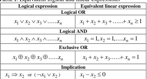
[image:1.595.307.547.659.788.2]Solving a discrete optimization problem involves two steps viz. modeling and solution search. Further discrete optimization problems may have purely logical entities or mixed logical and continuous entities. Three methodologies covering these aspects are cited, viz the MILP, GDP and MLLP. For casting the logic constrained problem as a standard MILP problem, binary variables are used to model decisions having values as TRUE or FALSE. Methods for systematically converting the logical relations involving the binary decisions to a constraint form are given by Cavalier et al. [1] and Mitra et al. [4]. Broadly, the methods involve either (a) converting each type of logical relation directly to an equation form using a standard lookup table giving the equations for each type of logical relationship or (b) transforming a proposition to a conjunctive normal form (CNF) or a disjunctive normal form (DNF) and deriving constraints based on these. For the case involving mixed logical and linear constraints, two methods, the Big M constraints and the convex hull using disaggregated variables are used as shown by Raman and Grossmann [7]. Table I gives various commonly occurring logical relation names, their logical expressions and their equivalent equation forms.
Table I: Equivalent logical and linear expressions Logical expression Equivalent linear expression
Logical OR
n x x x
x1 2 3... x1x2x3...xn1
Logical AND
n x x x
x1 2 3... x11,x21,...xn1
Exclusive OR
n x x
x
x1 2 3... x1x2x3...xn1
Implication
2 1 x
x or (x1x2) x1x2 0
Extended Formulations for Representation of
Logic Based Optimization Problems
Dhananjay Karandikar, K.P.Madhavan
The B&B or B&C solver technique of progressing through the search may not always be the best strategy in solution search. Rather, integer variables can be managed separately, allowing them to take only integer values. Modeling techniques other than MILP involve treating the discrete decisions as logical identities and apply logical processing methods on these identities. Logical inference methods and (or) constraint programming are used to process the logical identities. Continuous variables are processed using mathematical techniques. The Generalized Disjunctive Programming (GDP) model developed by Raman and Grossman [7] after papers handling logic in optimization [5], [6] and the Mixed Logical Linear programming (MLLP) model by Hooker and Osorio [3] are examples of this approach. These logic based techniques are designed with a motivation to reduce the solution time, notably by separating concerns for logical and continuous variables, as also giving a formal model for the optimization problem statement.
This paper describes techniques for modeling OLE using MILP so as to remove limitation of CLE. The methods given in Table I above are insufficient to model these requirements for MILP. It is possible though, to meet these requirements, using techniques given in section III below. It thus enables modeling of nested If-Then-Else conditions as declarative programs.
III. MODELING TECHNIQUES
The following sub-sections describe the modeling of various types of logical relations. In all the equations below, x1, x2, … xn are the input variables and z represents the result
of an expression. All the variables in this section below (along with any new subscripts added) are binary variables. If the logical expression is TRUE, then z gets set to a value of 1 else 0.
A. At Least m TRUE
The requirement here is to check if at least m of the n variables are TRUE. Equation (1) models the requirement.
1 ) 1 ( ... ... 3 2 1 3 2 1 m z m n x x x x mz x x x x n n (1) The first inequality in (1) forces z to be 0 if less than m variables are TRUE. The second inequality forces z to be 1 if m or more variables are TRUE.
B. At Max m TRUE with all 0 inclusive
The requirement here is to check if at max m of the n variables are TRUE. There are two cases possible for this condition, one being that when all inputs are 0, z should be 0 and the other case when even if all inputs are 0, z should still be 1. Equation (2) models the latter requirement. The former is seen in the next section.
m z m n x x x x z m x x x x n n ) 1 )( ( ... ) 1 )( 1 ( ... 3 2 1 3 2 1 (2) The first inequality in (2) forces z to be 1 if m or less variables are TRUE. The second inequality forces z to be 0 if more than m variables are TRUE.
C. At Max m TRUE with all 0 exclusive
The requirement here is to check if at max m of the n variables are TRUE. Equation (3) models the requirement. An auxiliary variable z2 is used here and also requires more
constraints. 1 ) 1 ( ... 1 ... ) 1 )( ( ... ) 1 )( 1 ( ... 2 2 3 2 1 2 3 2 1 3 2 1 2 3 2 1 z z z n x x x x z x x x x m z m n x x x x z z m x x x x n n n n (3)
For the “At max m true with all 0 exclusive” case, the value of z v/s the number of TRUE variables is a non-monotonic function. It is 0, when all the variables are 0, then 1 till m variables are TRUE and then 0 if more than m variables are TRUE. To model this, a superposition principle is employed. The condition that all variables are FALSE is detected in the variable z2. The value of this is
subtracted from z, required only for the case where it is to be enforced to 0 in the inequality 1.
D. Exactly equal to m
) ), (( ) 5 integers negative -non are 2 , 1 ) 4 ) 1 ( 2 1 ) 3 ) 1 ( 2 1 ) 2 2 1 ... 3 2 1 ) 1 m m n Max C y y z y y z C y y y y m n x x x x (4)
y1 and y2 are positive integer variables. Under any
condition, only one of these can be positive. Constraints 2 and 3 in (4) detect if y1 or y2 is positive and sets z to 0. If y1
and y2 are both 0, constraint 3 enforces z to 1. Thus z
becomes 1 only when summation is equal to m else it remains 0.
E. OR Logic
The OR logic states that if any one of the variables is TRUE then the result is TRUE else FALSE. The equivalent equation form of this proposition is given by the following methods. Equation (5) gives the method by Williams, after generalizing it from two variables to n variables, (Cavalier et.al. [1] call this as the substitution method).
0 .... 0 0 ... 2 1 2 1 z x z x z x z x x x n n (5)
The first constraint in (5) is active when all the input variables are 0. These enforce z to be 0. The rest of the constraints are active when that particular variable is 1. It enforces z to be 1.
Another method is given in (6).
when any one of the inputs is 1and enforces z to be 1. The substitution method will generate tighter bounds in the branch and bound solution method at the cost of additional constraints. It is straightforward to generate the NOR constraints from (5) and (6) above just by replacing z by 1-z. A generalization of (6) is the condition that at least m of the n variables should be TRUE which was discussed in section A. If value of m is set to 1 in (1), it becomes the OR Logic
F. And Logic
The AND logic states that for the output to be TRUE, all the inputs should be TRUE. Equation (7) is a method by Williams [8] after generalizing it for n inputs.
0 ....
0 0
1 ...
2 1
2 1
z x
z x
z x
n z x x
x
n
n
(7)
The first constraint in (7) is active when all the inputs are 1 and enforces z to be 1. The remaining constraints are active when the input is 0, which enforces the output to 0.
The AND logic can also be expressed with the following constraints.
1 ...
...
3 2 1
3 2 1
n z x x
x x
nz x x
x x
n n
(8) In (8), the first constraint is active when not all the variables are 1, and enforces z to be 0. The second constraint is active when all the variables are 1 and enforces z to be 1. Please note that the AND logic is a generalization of (1) with mset to n.
G. Exclusive OR
The Ex-Or is a special case of (4) as described in section D (Exactly equal to mTRUE), with mset to 1 or B (At max m TRUE), again with m set to 1.
H. Notation
For expressing any of the logical relations mentioned above, a letter ‘C’ is added to the relationship name to indicate a ‘Comprehensive’ relationship, i.e. one which is not constrained to be TRUE only. For example CAND indicates a ComprehensiveAND relationship and is different from the AND relationship given in Table I.
IV. APPLICATION
A. Application to a Production Scheduling Problem
This section shows the application of the above proposed methods for extending features of a problem in production planning, known as the Continuous Setup Lot-sizing and Scheduling Problem (CSLP) described by Drexl and Kimms in [2]. First, the important features of the CSLP are mentioned and in the subsequent section, the extended CSLP model is described.
a) It is a small bucket problem with only one product allowed per time slot.
b) The quantity of the production per time slot can be any value within the prescribed capacity constraints.
c) Switching cost between products is considered as a part of the objective function
d) This is different than the Discrete Lot-Sizing and Scheduling Problem (DLSP). In the DLSP, either no production happens in a time slot or it is to the full capacity.
1) The extended CSLP optimization model
Following are details of the production planning activity for the problem type considered here:
a) A single workstation manufactures multiple discrete products.
b) Capacity allocation should be done to meet the specified demand to the maximum possible value.
c) If switching occurs between products within a family, no setup cost or time is spent.
d) The switching state should be carried forward if the workstation is idle in between two products of the same family.
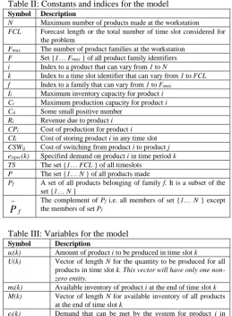
[image:3.595.296.556.359.712.2]Table II lists the various constants and Table III lists the variables used for the model.
Table II: Constants and indices for the model Symbol Description
N Maximum number of products made at the workstation FCL Forecast length or the total number of time slot considered for
the problem
Fmax The number of product families at the workstation F Set {1… Fmax } of all product family identifiers i Index to a product that can vary from 1 to N
k Index to a time slot identifier that can vary from 1 to FCL f Index to a family that can vary from 1 to Fmax
Ii Maximum inventory capacity for product i Ci Maximum production capacity for product i Cii Some small positive number
Ri Revenue due to product i CPi Cost of production for product i CIi Cost of storing product i in any time slot CSWij Cost of switching from product i to product j eispec(k) Specified demand on product i in time period k TS The set {1… FCL } of all timeslots
P The set {1… N } of all products made
Pf A set of all products belonging of family f. It is a subset of the
set {1… N }
f
P
~ The complement of Pf i.e. all members of set {1… N } except
the members of set Pf
Table III: Variables for the model Symbol Description
ui(k) Amount of product i to be produced in time slot k U(k) Vector of length N for the quantity to be produced for all
products in time slot k. This vector will have only one non-zero entity.
mi(k) Available inventory of product i at the end of time slot k M(k) Vector of length N for available inventory of all products
at the end of time slot k
ei(k) Demand that can be met by the system for product i in
time slot k, and can range from 0 to the target eispec(k) E(k) Vector of length N for the demand actually met ei(k), in
time slot k.
sORf(k) A binary variable used for the switching logic and has a
Symbol Description
sNORf(k) An intermediate binary variable used in the switching logic
and has a value of 1 if any family other than family f does not produce anything in time slot k.
sANDf(k) An intermediate binary variable used in the switching logic
and has a value of 1 if sNORf(k) and sORf(k-1) are both 1. swANDij(k) Switching variable between family i and family j at time
slot k.
Mass Balance Equations
Mass balance equations are the basis of developing a predictive model. Assume the inventory at the output for any product at the end of a period k is given by m1(k). Let u1(k)
be the amount of product produced in period k, e1(k) be the
demand or material drawn from the inventory. Equation (9) describes the basis of derivation for the mass balance relations for the product.
) ( ) ( ) 1 ( )
( 1 1 1
1k m k u k e k
m (9)
Using the same concept for future time periods, and aggregating the above equation for all the products at the workstation, the predictive model for the entire system till the Nth period is shown in (10). The matrices A, B and D are
the coefficients of m(k),u(k)and e(k) respectively.
Concisely this is represented as follows:
) ( ) ( ) 1 ( ) ( ~ ~ ~ ~ k E D k U B k M A k
M (10)
Capacity constraints for components
The total capacity requirement by all products taken together should not exceed the available capacity of the workstation in any time slot. The relations are shown in (11).
TS k C k u TS k C k u TS k C k u N
N
) ( ... ) ( ) ( 2 2 1 1 (11) Demand Constraints
The demand value is considered a decision variable here. Value for a demand on a product will be specified. Due to capacity constraints, it may not be possible to meet all the specified demand. This variable should lie within 0 at a minimum and the specified demand value at a maximum as shown in (12) and (13).
TS k P i k
ei( )0 , (12)
TS k P i k k
ei( )eispec( ) , (13)
Big M Constraints
These are used to detect if production for a particular product in a particular time slot is done or not. Upper and lower bounds are set as shown in (14) and (15). The lower bound may be required if this problem is for non-discrete systems to ensure that uib does not remain 0 when production
is 0. The binary variable is used as an indicator variable for conveying the TRUE or FALSE state of production.
} 1 , 0 { ) ( , , ) ( ) ( k u TS k P i k u C k u ib ib i i (14) } 1 , 0 { ) ( , , ) ( ) ( k u TS k P i k u k u C ib i ib ii (15)
One product Constraints
These are used to limit the production to only one product per time slot. The constraint, as shown in (16) is an inequality constraint since there need not be any product scheduled for production in the time slot.
} 1 , 0 { ) ( , 1 ) ( 1
k u TS k k u ib N i ib (16) Switching ConstraintsLogic to meet the switching requirements is described in the following steps:
1) Define a variable sORf(k), for each family f in each time slot k, which is true if any of the following two conditions are true, expressed in (17) to (20) below. a. Any product in family f for a particular time slot is
scheduled
b. There are two clauses to this second conditional statement and are given below:
i. No product in any other family (indicated by Ff
~
in (17) below) for a particular time slot is scheduled, sNORf(k), AND
ii. Any product in the family f in the previous time slot is scheduled, sORf(k-1).
The result of the two clauses is the value of the variable sANDf(k). Considering the fact that (16) states that at a maximum only one product can be scheduled, it may so happen that in a particular time slot, there is no product being scheduled at all. The additional condition, b, is added to carry forward the state of the previous time slot if there is no production in the current timeslot. For doing this, it is first necessary to verify that any other family product is not being produced. Further it is also necessary to check if the same family was true (not necessarily being produced since the state might be carried forward from its previous time slot) in the previous time slot.
} 1 , 0 { ) ( , } .... 2 { , )) ( ( ) ( ~ k sNOR FCL k F f k u CNOR k sNOR f ib F i f f (17) } 1 , 0 { ) ( ), ( ), ( }, .... 2 { , )) 1 ( ), ( ( ) ( k sOR k sNOR k sAND FCL k F f k sOR k sNOR CAND k sAND f f f f f f (18) } 1 , 0 { ) ( ), ( , } .... 2 { , )) ( ), ( ( ) ( k sAND k sOR FCL k F f k sAND k u COR k sOR f f f ib F i f f (19) } 1 , 0 { ) ( 1 , )) ( ( ) ( k sOR k F f k u COR k sOR f ib F i f f (20)
2) Define switching between consecutive time slots between families using AND logic. A binary switching variable swANDij(k) shows the switching status between
this variable has a value of 1, then this switching has occurred else not. This is expressed as follows in (21):
} 1 1 {
)) 1 ( ), ( ( )
(
...FCL-F, k
i,j
k sOR k sOR CAND k
swANDij i j
(21)
Minimum and Maximum constraints on the input:
The minimum value for any input variable is 0 and the maximum value is the production capacity of the workstation for that product as described in (22) and (23).
TS k P i C k
ui( ) i , (22)
TS k P i k
ui( )0 , (23)
Minimum and Maximum constraints on inventory
Minimum constraint on the inventory is 0 and the maximum constraint is the inventory capacity for that product. More complex scenarios like shared inventory capacity within all products is not considered for convenience. These constraints are shown in (24) and (25).
TS k P i k
mi( )0 , (24)
TS k P i I k
mi( ) i , (25)
Objective Function
The objective is to maximize the profit which is the difference between the revenue and the cost due to operations. Equation (26) gives the calculation.
) ( *
)] ( * ) [(
) ( *
max
max max
1 1 1 1 1
k swAND CSW
k u CI CP k e R rev
ij F
i F
j FCL
k ij
i i i N
i FCL
k i i
(26)
2) Some observations about the model
a) At least one method to model the same requirements without using the developments mentioned in this paper can be depicted. Instead of modeling the switching cost between families, a switching between individual products can be modeled. The switching matrix will have a bigger size. Further the number of variables used to model the switching will also be of the order of n2,
where n is the number of products. In the model developed here the switching variables reduce and are of the order of f2, where f is the number of families and
in most cases will be much less than n. Thus this method reduces the number of variables required for modeling. b) An example of the possibilities based on the outcome of
the logical relation being modeled as part of the problem can be cited. The values of sORf for any two
consecutive time slots are taken which can be 0 or 1. These values affect the value of the switching variable sANDij, and are modeled as part of the problem itself.
c) Switching in CSLP has a loose formulation. The value of xjt as shown by Drexl and Kimms in [2] can have a
value of 1 when there is a positive difference between the yjt and yj(t-1) . But it can also be 1 when these two are
equal and not indicating a switching condition, and specifically when no production is being done in that time slot. This is due to the inequality constraints. The model presented here is a tighter formulation with switching modeled to be true only when it truly occurs.
3) Simulation and Results
The above model was implemented in MATLAB. After the problem is formulated, a call is made to an MILP optimizer. Two freeware solvers viz. COIN CBC and LPSolve were used for this purpose. Two solvers were used to verify the consistency of the results.
Two test cases with different input data were considered and are shown below in tabular form. For each test case, details of the input data are given and then results are shown along with a discussion on the results. The objective of both the test cases is to maximize the profit of the system, which is defined to be a difference between the revenue and cost. In the first test case the demand is much greater than the available capacity. The aim is to check the products selected and sequence of their allocation. In the second case, the demand is much less than the available capacity. Here the aim is to check the sequence and time slots where the products are allocated as also the carryover of the switching state during idle time.
Setup Details
a) The workstation produces seven different types of products. Products are identified serially by alpha-numeric characters P1 to P7.
b) All products are discrete type.
c) There are three families within the products. Products P1 to P3 belong to family 1, products P4 and P5 belong to family 2 and products P6 and P7 belong to family 3. Families are identified serially by alpha-numeric characters F1 to F3.
d) Time slots are used to model the problem as described above. Six time slots are used for the cases below. These are identified by alpha-numeric characters T1 to T6.
e) There is no cost for switching from one product to another within a family. The cost of switching from one product to another between families has a cost and is given in the data for the test cases below.
f) Among the various parameters, production capacity and inventory capacity are considered to have the same values across all time slots. Specified demand, production cost, inventory cost and revenue, which have a direct impact on the profitability, are kept different.
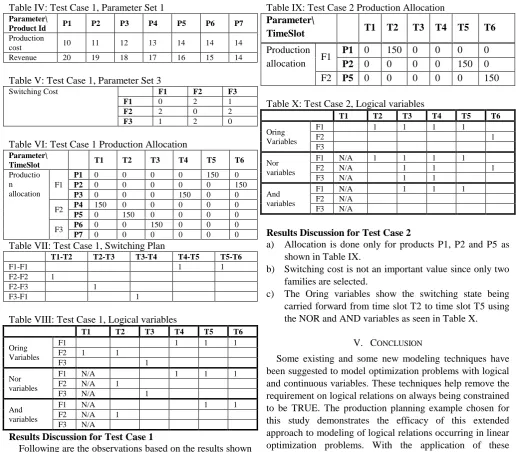
Test Case 1
Table IV: Test Case 1, Parameter Set 1 Parameter\
Product Id P1 P2 P3 P4 P5 P6 P7
Production
cost 10 11 12 13 14 14 14
Revenue 20 19 18 17 16 15 14
Table V: Test Case 1, Parameter Set 3
Switching Cost F1 F2 F3
F1 0 2 1
F2 2 0 2
F3 1 2 0
Table VI: Test Case 1 Production Allocation Parameter\
TimeSlot T1 T2 T3 T4 T5 T6
Productio n allocation
F1
P1 0 0 0 0 150 0
P2 0 0 0 0 0 150
P3 0 0 0 150 0 0
F2 P4 150 0 0 0 0 0
P5 0 150 0 0 0 0
F3 P6 0 0 150 0 0 0
P7 0 0 0 0 0 0
Table VII: Test Case 1, Switching Plan
T1-T2 T2-T3 T3-T4 T4-T5 T5-T6
F1-F1 1 1
F2-F2 1
F2-F3 1
F3-F1 1
Table VIII: Test Case 1, Logical variables
T1 T2 T3 T4 T5 T6
Oring Variables
F1 1 1 1
F2 1 1
F3 1
Nor variables
F1 N/A 1 1 1
F2 N/A 1
F3 N/A 1
And variables
F1 N/A 1 1
F2 N/A 1
F3 N/A
Results Discussion for Test Case 1
Following are the observations based on the results shown in Table VI, Table VII and Table VIII:
a) Allocation is done only for products P1 to P6.
b) The switching happens from family 2 to family 3 then to family 1. This sequence adds the least switching cost. Table VII shows only those rows which indicate a switching.
c) Considering the lack of capacity as compared to the demand, product P7 demand is not met because this gives the least profit.
d) The logical variable values are shown in Table VIII. The Oring variables for appropriate families have a value of 1 which corresponds to the production variable values shown in Table VI.
e) The NOR and AND variables do not have much significance in this test case since there are no empty slots. Nevertheless, their values are as expected.
Test Case 2
For this test case, a nominal inventory cost of 1 unit is considered for all the products across all timeslots. Demand of 150 units is considered each only for P1 in timeslot 2, P2 by timeslot 6 as also P5 by timeslot 6. All other products have no demand, making the demand in the system much less than the available capacity.
Table IX: Test Case 2 Production Allocation
Parameter\
TimeSlot T1 T2 T3 T4 T5 T6
Production allocation F1
P1 0 150 0 0 0 0
P2 0 0 0 0 150 0
F2 P5 0 0 0 0 0 150
Table X: Test Case 2, Logical variables
T1 T2 T3 T4 T5 T6
Oring Variables
F1 1 1 1 1
F2 1
F3
Nor variables
F1 N/A 1 1 1 1
F2 N/A 1 1 1
F3 N/A 1 1
And variables
F1 N/A 1 1 1
F2 N/A F3 N/A
Results Discussion for Test Case 2
a) Allocation is done only for products P1, P2 and P5 as shown in Table IX.
b) Switching cost is not an important value since only two families are selected.
c) The Oring variables show the switching state being carried forward from time slot T2 to time slot T5 using the NOR and AND variables as seen in Table X.
V. CONCLUSION
Some existing and some new modeling techniques have been suggested to model optimization problems with logical and continuous variables. These techniques help remove the requirement on logical relations on always being constrained to be TRUE. The production planning example chosen for this study demonstrates the efficacy of this extended approach to modeling of logical relations occurring in linear optimization problems. With the application of these techniques the range of the problems that can be modeled can be widened.
REFERENCES
[1] T. M. Cavalier., P. M. Pardalos and A. L. Soyster, (1990). Modeling and integer programming techniques applied to propositional calculus, Computers Opns Res., Vol. 17, No. 6. 561-570
[2] A. Drexl, A. Kimms, (1997). Lot sizing and scheduling - Survey and extensions, European Journal of Operational Research99, 221-235 [3] J. N. Hooker, and M. A. Osorio, (1999). Mixed logical/linear
programming, Discrete Applied Mathematics 96-97, 395-442 [4] G. Mitra, C. Lucas, S. Moody, E. Hadjiconstantinou, (1994). Tools
for reformulating logical forms into zero-one mixed integer programs, European Journal of Operational Research 72, 262-276
[5] R. Raman, I.E.Grossmann, (1991). Relation between MILP modeling and logical inference for chemical process synthesis, Computers and Chemical Engineering 15, 73-84.
[6] R. Raman, I.E.Grossmann, (1993). Symbolic Integration of logic in Mixed-Integer Linear programming techniques for process synthesis, Computers and Chemical Engineering 17, 909-927
[7] R. Raman, I.E.Grossmann, (1994). Modeling and computational techniques for logic based integer programming, Computers and Chemical Engineering 18, 563-578
[8] H. P. Williams, (1985). Model Building in Mathematical Programming, 2nd edn. Wiley, New York