The bifurcation structure of a thin superconducting loop
with small variations in its thickness
G. Richardson
∗January 18, 2007
Abstract: We study bifurcations between the normal and superconducting states, and between
superconducting states with different winding numbers, in a thin loop of superconducting wire, of uniform thickness, to which a magnetic field is applied. We then consider the response of a loop with small thickness variations. We find that close to the transition between normal and superconducting states lies a region where the leading order problem has repeated eigenvalues. This leads to a rich structure of possible behaviours. A weakly nonlinear stability analysis is conducted to determine which of these behaviours occur in practice.
Keywords: Little-Parks experiment, superconductivity.
1
Introduction
Certain materials when cooled sufficiently undergo a second order phase transition which takes them from the normal state, in which they behave like conventional metals, to a state in which electric currents can be supported without resistance and in which unusual mag-netic phenomena are exhibited. This state, termed the superconducting state, is one of the few examples where quantum mechanics manifests itself over a macroscopic scale. Indeed it is possible to attribute many of the peculiar properties of superconductors directly to the quantum mechanical nature of the phenomenon. In this context we note (I) the Josephson effect whereby two pieces of superconducting material separated by a non-superconductor interact via quantum mechanical tunelling, and (II) the quantisation of magnetic flux ex-emplified by a circulating current structure, termed a vortex, which is associated with one quantum of magnetic flux.
In this work we shall investigate, from a theoretical standpoint, the famous Little–Parks experiment [4] and other closely related set-ups. The inventors of this experiment used an extremely thin hollow cylinder to which an axial magnetic field is applied to show that the transition temperature at the onset of superconductivity has a periodic dependence on the
flux within the ring. By noting that an integer plus-half-number of magnetic flux quanta within the ring penalises the superconducting state in comparison to an integer number of quanta, they argue that the period of variation in the transition temperature is exactly one quantum of magnetic flux. Recently there has also been considerable interest in a closely related set-up consisting of a thin closed loop of wire set in an applied magnetic field (see for example Fomin et al. [5] and Moshchalkov et. al. [6].)
Interest in the Little Parks experiment has not been solely restricted to experiment and much work has been done on the problem from a theoretical standpoint. In [3] the normal-superconducting transition is investigated by application of the Ginzburg-Landau model to a thin circularly-symmetric annulus. The work of Berger and Rubinstein [1] extends that performed in [3] with the discovery of a further set of transition lines between different superconducting solutions. It also investigates the effects that variations in the thickness of the ring have on the phase diagram, revealing novel symmetry breaking effects. Approximate one-dimensional Ginzburg-Landau models for a non-circularly-symmetric thin ring and a three dimensional thin loop of wire with varying thickness have been derived in [7] and [8] respectively and may be used to investigate the Little–Parks effect in non-circularly symmetric domains.
The present work is an extension of that performed by Berger and Rubinstein in [1]. We find that by formulating the problem in a different manner from these authors we are able to build up a detailed picture of the bifurcation structure of the problems, describing: (I) a thin ring or loop with uniform thickness, and (II) a thin ring or loop with small variations in the thickness. In the next section we formulate the problem for a thin wire of arbitrary geometry. In Section 3 we consider a loop of uniform thickness and describe the local behaviour of the system in the neighbourhood of the normal-superconducting bifurcation line, and in the neighbourhood of the transition lines between superconducting solutions with different topological winding numbers. In Section 4 we extend the analysis of the previous section to a wire with small variations in its thickness. In this section we also conduct a detailed analysis about the points in the phase diagram where the bifurcation lines intersect and where the symmetry breaking discovered in [1] is most marked. Finally, in Section 5, we draw our conclusions.
2
Problem Formulation
In the following we consider a loop of thin wire of length 2πl and with a typical cross sectional area η (where η 1) lying along the curve x = q(s).1 Our starting point is the
1We also require thatηlξwhereξ is the coherence length. In effect this amounts to requiring that the
Ginzburg-Landau equations [2]
1
ms (~∇ −iesA)
2
Ψ = a(T)Ψ +b(T)|Ψ|2Ψ,
∇ ∧
B
µ
= −ies~
ms (Ψ
∗
∇Ψ−Ψ∇Ψ∗
)− 2e
2
s ms|Ψ|
2A,
∇ ∧A = B.
Here Ψ is a complex order parameter for the superconducting charge carriers, B is the magnetic field, T is the temperature and es and ms are respectively the charge, and the effective mass of the superconducting charge carriers. We take the magnetic flux enclosed by the ring to be of the order of one flux quantum, and employ the nondimensionalisation
x∼l Ψ∼
s
|a(T)|
b(T) B ∼ ~
esl2 A∼
~
esl.
Following the analysis presented in [7] then leads to a one dimensional model for the averaged (over the thickness of the wire) order parameterψ as a function of the dimensionless distance along the loop s
∂ ∂s −iA
2
ψ+|Γ|(sgn(Γ)− |ψ|2)ψ+D
0
(s) D(s)
∂ψ
∂s −iAψ
= 0. (1)
In the above D(s) is the cross-sectional area of the loop scaled with η,Ais is the component of the vector potentialAtangential to the curvex=q(s), and Γ is a temperature-dependent parameter defined by
Γ = 1 ξ2 =
−l22ma
~2 .
Close to Tc, the critical temperature below which superconducting state is energetically favourable in the absence of magnetic field, Γ can be approximated by Γ =k(Tc−T) where k is a positive constant. Remarkably this model is entirely independent of the geometry of the wire and depends on the magnetic field solely through the magnetic flux cutting the loop. Indeed, if we select a gauge for A such that its tangential component along the wire is constant we find A is related to F as follows:
A= F 2π.
is derived in [7] and, where we employ the same nondimensionalisation as above, may be written as follows:
−|Γ|
∂ψ
∂t +iΦψ
+
∂ ∂s −iA
2
ψ+ 1 D
∂D ∂s
∂ψ
∂s −iAψ
− |Γ|ψ |ψ|2−sgn(Γ)
= 0, (2)
∂ ∂s
D
|ψ|2A+ i 2
ψ∗∂ψ
∂s −ψ ∂ψ∗
∂s
+σ ∂ ∂s D ∂Φ ∂s + ∂A ∂t
= 0, (3)
where Φ is the dimensionless scalar electric potential. It is sometimes convenient to replace (3) by
|Γ|i 2
ψ∂ψ
∗
∂t −ψ
∗∂ψ
∂t
+|Γ||ψ|2Φ = σ D ∂ ∂s D ∂Φ ∂s + ∂A ∂t . (4)
which is easily derived from (2)-(3).
3
A loop with uniform thickness
D
≡
1
Equation (1) has the solution ψ = 0 which corresponds to the normal state. We search for a bifurcation from this solution to a superconducting solution by linearising about ψ = 0 as follows:
ψ =ψ1+· · · 1.
and substituting into (1). At O() we find thatψ1 satisfies the linear equation
LΓψ1 =
∂2ψ 1
∂s2 −2iA
∂ψ1
∂s −A
2ψ
1+ Γψ1 = 0, (5)
with periodic boundary conditions on [0,2π]. This has the non-trivial eigensolution
ψ1 =Eeims for Γ = (m−A)2,
where m is an integer. Hence as Γ increases from zero the first solution to bifurcate is that with winding number nint(A), where we define nint(A) to be the integer closest to A. In fact we can extend the solution (6) to all values of Γ >(m−A)2 and hence to |ψ| = O(1)
by noting that
ψ =γeims |γ|2 = sgn(Γ)− (m−A)
2
|Γ| , (6)
3.1
Linear stability of the normal solution
It is important to distinguish between branches of this bifurcation which correspond to stable solution, and are thus observable, and those which correspond to unstable solutions. We begin by investigating the linear stability of the normal solution by expanding about ψ = 0 in powers of (1)
ψ = eαtψ1(s) +O(2),
Φ = O(2),
and then substituting this expansion into the time dependent model (2)-(3). At 0() we find
−α|Γ|ψ1+LΓψ1 = 0, ψ1(0) =ψ1(2π), ψ 0
1(0) =ψ 0 1(2π).
This has solutions of the form
ψ1,m =eims αm = sgn(Γ)−
(m−A)2
|Γ| ,
where m is an integer. Hence one can see that small perturbations to the normal state will in general grow if we can find an integer m such that (m−A)2/Γ<sgn(Γ).
3.2
Linear stability of the superconducting state with winding
number
m
The stability of the steady superconducting solution ψ = γeims can be investigated in a similar manner. We make the following expansion about this solution:
ψ = γeims+eαtψ1(s) +· · · ,
Φ = eαtΦ
1(s) +· · · .
Making the assumption thatγ is real (with no loss of generality) and substituting the above expansion into (2) and (3) we find, at O(),
ˆ LΓψ1 =
∂2ψ 1
∂s2 −2iA
∂ψ1
∂s −A
2ψ
1+ Γ(1−2|γ|2)ψ1−Γγ2e2imsψ ∗
1 = Γ αψ1 +iγeimsΦ1
, (7)
A−m
2
eimsψ1 ∗
+e−ims
ψ1
+ i
2
e−ims∂ψ1
∂s −e
ims∂ψ1 ∗
∂s
+σ γ
∂Φ1
∂s =F, (8)
where F is an arbitrary constant. We look for periodic solutions of the form
ψ1,j = eims bjeijs+b−je −ijs
, Φ1,j = i djeijs+d−je
wherej is a non-zero integer. Substitution of the above into (7) and (8) leads to the following equations for (bj, b−j) and (dj, d−j):
Γγdj = Γγ2b∗
−j +Pjbj =Njbj −N−jb ∗
−j, (9)
where
Nj = Γγ2
σj
A−m− j
2
and Pj = ((m+j)−A)2+ Γ(2γ2−1 +α).
By making the transfromation j → −j in (9) we find a relation between b−j and b ∗
j. Then, on use the definition of γ found in (6), we can show that these relations are consistent only if α, the growth factor, is a solution to the quadratic
Γ2α2 + Γα
Γγ2
σ + 2j
2+ 2 Γ−(m−A)2
+
j2+ Γγ
2
σ
j2 −6(m−A)2+ 2Γ = 0.
Since Γ ≥ (m−A)2 the coefficient multiplying α in the equation above must be positive.
Hence solutions α of this quadratic have positive real part iff 6(m−A)2−2Γ−j2 >0. The
winding number msolution to (1)ψ =γeims is thus unstable for values of Γ and αfor which
fm(Γ, A) = 6(m−A)2−2Γ−1>0.
We must now investigate the case j = 0. Here we find a solution to (7)-(8), valid for all Γ and A2,
ψ1 =iEeims Φ1 = 0 α= 0 E ∈R. (10)
It follows that the winding number m solution to equation (1) ψ = γeims is only neutrally stable for {(Γ, A) :fm(Γ, A)<0}. This should cause little surprise since ψ = γeims+ν is a steady solution to (1) for all real ν. The reader should note that a change in phase of the solution makes no difference to the observable quantities of the system and does not alter the conclusions we draw in this work.
3.3
Bifurcation between superconducting states with different
wind-ing numbers
In§3.2 above we saw that the winding numbermsolution to (1)ψ =γeims becomes unstable for 3(m−A)2−1/2>Γ. One can associate the loss of stability with a bifurcation occuring
on Γ = 3(m−A)2−1/2. In order to investigate the bifurcation further we look for a steady
solution to (1) of the form
(b) u
dC dτ <0 s
dC dτ >0
u Γ
(a)
|γ|
u s
s
Γ2
C
u dC
dτ >0
[image:7.595.99.497.106.287.2]dC dτ <0
Figure 1: Bifurcation diagrams for (a) the normal-superconducting transition (b) the onset of instability of the superconducting solution
At first order we find the following equation for ψ1:
ˆ
LΓψ1 = 0, (11)
together with periodic boundary conditions on [0,2π]. By comparison with§3.2 above we can immediately see that this problem has eigenvalue Γ = 3(m−A)2−1/2. The corresponding
eigenvector is
ψ1 =Ceims(2i(m−A) sin(s−ν)−cos(s−ν)) C, ν ∈R.
We now seek to determine the dependence of C, the amplitude of ψ1, on small deviations
in Γ away from the eigenvalue of (11) by proceeding to higher orders in the expansions ofψ and Γ
ψ = ψ0+ψ1+2ψ2 +3ψ3+· · · ,
Γ = Γ0 +2Γ2+3Γ3+· · · .
where
ψ0 =γ0eims, ψ1 =Ceims(2i(m−A) sin(s−ν)−cos(s−ν)),
and
gm =m−A, Γ0 = 3gm2 −1/2, γ0 =
1− g
2
m (3g2
m−1/2) 1/2
. (12)
At O(2) we find the following equation for ψ 2
ˆ
LΓ0ψ2 =H(s) =−Γ2ψ0(1− |ψ0|
2) + Γ
0 2ψ0|ψ1|2+ψ0 ∗
ψ1ψ1
together with periodic boundary conditions on [0,2π]. Since nontrivial solutions exist to the homogenous problem
ˆ
LΓ0w= 0 w periodic on [0,2π], (14)
we can use the Fredholm alternative to find a solvability condition on the right-hand side of (13); this is
Re Z 2π
0
H(s)w∗
ds
= 0 ∀ w satisfying (14). (15)
The right-hand side of (13) satisfies (15) for allC and ν; we therefore solve forψ2 to find
ψ2 =γ0eims C2(iM2sin(2s) +M1cos(2s)) +h1+h2C2
+P ψ1
where
M1 =
3Γ0
2(6g2
m−2Γ0−4)
, M2 =gm(Γ0/2−M1),
h1 =
Γ2gm2 2Γ0(Γ0−gm2)
, h2 =
Γ0(3/2 + 2gm2) 2(g2
m−Γ0)
,
and P is an arbitrary constant. Proceeding to O(3) we find the following equation forψ 3
ˆ
LΓ0ψ3 =
Γ0(|ψ1|2ψ1 + 2ψ0ψ1ψ2 ∗
+ 2ψ0ψ2ψ1 ∗
+ 2ψ1ψ2ψ0 ∗
)+ Γ2((2|ψ0|2−1)ψ1+ψ0ψ0ψ1
∗
)−Γ3(1− |ψ0|2)ψ0
. (16)
together with periodic boundary conditions on [0,2π]. Applying the solvability condition (15) to equation (16) leads to the following relation between Γ2 and C
C(C2(18g2m−3)(4gm2 + 1)−4Γ2) = 0. (17)
The coefficient multiplying C3 is positive since g2
m >1/4. The bifurcation diagram resulting from (17) is thus qualitatively similar to the picture in figure 1b.
3.4
Weakly nonlinear stability analysis of the bifurcation from the
superconducting solution with winding number
m
In the vicinity of this bifurcation, the linear stability analysis carried out in§3.2 reveals that all single wavenumber perturbations to the solutionψ =γeims decay exponentially in time t with the exception of the zero’th mode, which is always neutrally stable, and the first mode
At leading order the latter has zero growth rate α. In order to investigate the stability of perturbations of this form in the neighbourhood of the bifurcation one needs to conduct a weakly nonlinear stability analysis. This we do by introducing the long time scale τ = t and looking for a solution to the time-dependent model of the form
ψ = γeims +C(τ)eims(2i(m−A) sin(s−ν)−cos(s−ν)) +2ψ2+3ψ3· · · ,
Φ = 3N(τ)φ3(s) +· · · .
By adopting an approach similar to that employed in§3.3 we were able to find an expression for dC/dτ. As expected the lines upon which dC/dτ = 0 are those given by equation (17). They divide regions in which dC/dτ is positive from regions in which it is negative. The stability of a particular bifurcation branch depends on the sign of dC/dτ above and below it and the importance of the weakly nonlinear stability analysis is in identifying the sign of dC/dτ in the different regions. The results in this particular case are summarised figure 1b.
Remark It is nearly always possible to infer the sign of the growth rate of the most unstable mode (in this case dC/dτ) in some region from a linear stability analysis conducted along any two of the bifurcation branches. It follows that we can also infer the stability of the other bifurcation branches.
3.5
Description of the behaviour of the uniform ring
In §3 we examined the bifurcation structure of a thin ring with uniform thickness. It was found, that as Γ increases from zero, the normal solution first becomes unstable when Γ = (nint(A)−A)2 at which point a stable superconducting solution, of the form ψ = γeims (m = nint(A)) bifurcates from the normal solution (see figure 1a). We were also able to analyse the stability of the superconducting solution, with winding number m, far from the normal-superconducting transition. We found that this solution becomes unstable as the functionfm(Γ, A) = 6(m−A)2−2Γ−1, increases through zero at which point a subcritical
bifurcation occurs (see figure 1b). We expect that after the winding numberm solution loses stability the system will evolve to a solution with winding number m−1 orm+ 1 depending on whether fm−1(Γ, A) or fm+1(Γ, A) is negative. Physically this corresponds to a vortex
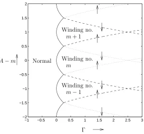
moving across the ring. These results are summarised in in the phase diagram plotted in figure 2. Here the solid line represents the normal-superconducting transition; the middle two dashed lines bound the region of stability of the solution ψ =γeims and the dotted lines bound the regions of stability of the solutionsψ =γei(m+1)s andψ =γei(m−1)s
−1 −0.5 0 0.5 1 1.5 2 2.5 3 −2
−1.5 −1 −0.5 0 0.5 1 1.5 2
A−m Winding no.
m
Winding no.
Winding no. m+ 1
m−1 Normal
[image:10.595.127.417.108.379.2]Γ
Figure 2: The phase diagram for a ring of uniform thickness
with higher energy than the global minimum. As the parameters of state move through some critical value there is a catastrophic loss of stability which sends the system into an equilibrium far from its original state. In common with other systems which exhibit superheating/supercooling we expect that where the system lies in the metastable state a sufficiently large perturbation may drive it out of this equilibrium into an equilibrium with lower energy.
In this context we also note the work of Zhang and Price [9] in which experimental evidence of this hysteresis is presented.
4
A loop with small variations in thickness
In this section we examine the effect that a small variation in the thickness of the ring has on the bifurcation structure of equation (1). We write D, the measure of the thickness, as follows:
and expandD1 as a Fourier series in s, choosing the origin of thes coordinate such that the
coefficient of sin(s) vanishes
D1(s) = ∞
X
n=1
βncos(ns) +
∞
X
n=2
αnsin(ns),
We substitute (18) into equation (1) and look for solutions. Clearly ψ ≡ 0 (the normal state) is still a solution. We can also find a superconducting solution by looking for a regular perturbation of the exact solution for a uniform ring (see equation (6)) of the form
ψ =γeims+δψ1+· · · , (19)
where
γ = 1−gm2/Γ1/2
. (20)
At O(δ) substitution of the above into (1) gives rise to the following equation forψ1:
ˆ
LΓψ1 =−igmD
0 1γeims.
together with periodic boundary conditions on [0,2π]. This problem has solution
ψ1 =−γgmeims ∞
X
n=1
βn 6g2
m−2Γ−n2
2gmcos(ns) +i(2g
2
m−2Γ−n2)
n sin(ns)
+
∞
X
n=2
αn 6g2
m−2Γ−n2
2gmsin(ns)− i(2g
2
m−2Γ−n2)
n cos(ns) !
. (21)
The regular expansion (19) breaks down close to the normal-superconducting transition as γ →0. For non-zero β1 this expansion also breaks down along the transition lines between
winding numbers. This is because the denominator of the first term in (21), 6g2
m−2Γ−1, vanishes. In§4.1, §4.2 and §4.3 we examine the effect that variations in the thickness of the wire have upon these bifurcations.
4.1
Normal-Superconducting transition
As (1−g2
m/Γ)1/2 decreases towards zero so does the amplitude ofψ. For sufficiently small ψ small deviations in the loop thickness directly affect the leading order behaviour of the order parameter. Scaling ψ appropriately will thus allow us to investigate the effect of the small thickness variations on the normal-superconducting bifurcation. As we shall demonstrate it is appropriate to scale ψ with δ; this motivates the following expansion:
ψ = δψ0+δ2ψ1+δ3ψ2+· · · ,
where Γ0 =gm2 (gmis defined in (12)). Substituting into (1) we find the leading order solution satisfies
LΓ0ψ0 = 0, (22)
together with periodic boundary conditions on [0,2π]. Since Γ0 =gm2 is an eigenvalue of (22) there is a nontrivial periodic solution, namely
ψ0 =Ceims C ∈C,
At O(δ2) we find an equation forψ 1
LΓ0ψ1 =−D
0 1(ψ
0
0−iAψ0), (23)
together with periodic boundary conditions on [0,2π]. Although the problem for ψ1 is an
inhomogenous version of the eigenvalue problem for ψ0, the inhomogeneity is such that we
can find a periodic solution forψ1; this is
ψ1 =Ceims ∞
X
n=1
βn n2−4g2
m
2gm2 cos(ns)−ingmsin(ns)
+
∞
X
n=2
αn n2−4g2
m
2gm2 sin(ns) +ingmcos(ns) !
+Rψ0,
whereR is an arbitrary constant. Proceeding toO(δ3) we find the following equation forψ 2:
LΓ0ψ2 =H(s) = D1D
0 1(ψ
0
0−iAψ0) + Γ0|ψ0|2ψ0−D 0 1(ψ
0
1−iAψ1)−Γ2ψ0, (24)
together with periodic boundary conditions on [0,2π]. This is, once again, an inhomogeneous version of the eigenvalue problem for ψ0 and, in order for it to have a periodic solution, we
require that the right-hand side satisfy the solvability condition
Z 2π
0
H(s)ψ0 ∗
ds = 0.
Applying this condition to (24) gives rise to the following relation between C and Γ2:
C = 0 or Γ2 =gm2 |C|2−
β2 1
2(1−4g2
m)
−
∞
X
n=2
n2(α2
n+βn2) 2(n2−4g2
m) !
. (25)
Providing g2
m 6= 1/4 the qualitative features of the bifurcation remain unchanged from those of the uniform ring (see figure 1a). Quantitatively one can see that the effect of the non-uniformity is to slightly decrease the value of Γ at which the bifurcation occurs (i.e at whichC = 0), although notably this critical value of Γ still has minimum value zero attained when gm =m−A = 0. Perhaps the most interesting feature of equation (25) is that where β1 6= 0 there is a singularity ofC at the points gm =m−A=±1/2. This is associated with
4.2
Transition between superconducting states with different
wind-ing numbers
We now procced to examine the effect of small variations in the thickness of the wire upon the transition between superconducting states with different winding numbers (these transitions are represented by dotted and dashed lines in the phase diagram plotted in figure 2). As in
§4.1 above we need to identify the size of the perturbation to the uniform solutionψ =γeims at which effects resulting from variations in the thickness of the wire are of the same order as those resulting from the proximity of the bifurcation. It turns out that the appropriate scaling for the perturbation ofψ is δ1/3; this motivates the following expansion:
ψ = ψ0+δ1/3ψ1 +δ2/3ψ2+δψ3 +· · · ,
Γ = Γ0+δ2/3Γ2+δΓ3+· · ·.
where
ψ0 =γ0eims, γ0 =
1− 2g
2
m 6g2
m−1 1/2
, Γ0 = 3gm2 − 1
2. (26)
Substituting the above into equation (1) we retrieve the same equations at first and second order (i.e O(δ1/3) andO(δ2/3)) for ψ
1 and ψ2 as we did in §3.3, namely (11) and (13). Upto
the constantsCandνthe solutions of these equations are the same as those in§3.3. However, since variation in the thickness of the wire is associated with a loss of symmetry, we can no longer expect the phase ν of ψ1 to remain completely arbitrary. It is thus more convenient
for our present purposes to write ψ1 and ψ2 in the form
ψ1 = Ceims(2igmsin(s)−cos(s)) +Eeims(2igmcos(s) + sin(s)),
ψ2 = γ0eims (C2−E2)(iM2sin(2s) +M1cos(2s)) + 2CE(iM2cos(2s)−M1sin(2s))
+h1+h2(C2+E2)
,
where C and E are real constants still to be determined and M1, M2, h1 and h2 are as
defined in §3.3. Proceeding to O(δ) we find the following inhomogenous equation forψ3:
ˆ
LΓ0ψ3 =
Γ0(|ψ1|2ψ1+ 2ψ0ψ1ψ2 ∗
+ 2ψ0ψ2ψ1 ∗
+ 2ψ1ψ2ψ0 ∗
)+ Γ2((2|ψ0|2−1)ψ1+ψ0ψ0ψ1
∗
)−Γ3(1− |ψ0|2)ψ0 −D 0 1(ψ
0
0−iAψ0)
. (27)
together with periodic boundary conditions on [0,2π]. In order to find a solution for ψ3 we
require the right hand side of (27) to satisfy the solvability condition (15). Applying this condition results in two coupled relations for C and E which are independent of αn, βn for n ≥2 ,
(C3+E2C)(72gm4 + 6gm2 −3) = 4β1
s 4g2
m−1 6g2
m−1
+ 4Γ2C,
It is straightforward to show that E = 0 and thus that
C3(18g2m−3)(4gm2 + 1)−4Γ2C = 4β1
s 4g2
m−1 6g2
m−1 .
The presence of the term on the right hand side of this equation, for β1 6= 0, is enough to
cause a qualitative change in the dependence of C on Γ2 from that found in the uniform
ring. Without loss of generality where β1 is non-zero we can set it equal to 1. Having made
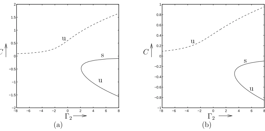
this simplification we plot C versus Γ2, for two values of gm, in figure 3. In accordance
with the remark made in §3.4 we can infer the stability of the bifurcation branches from our knowledge of the stability of the solution for large |Γ2| (see §3.1).
We can use the results obtained above to describe the transition from one winding number to an adjacent winding number in a slightly non-uniform ring. One can see that as Γ approaches the critical value 3(m−A)2−1/2 from above the perturbation to the solution
ψ = γeims, caused by the non-uniformity, grows from size O(δ) to O(δ1/3) until a certain
value of Γ is reached, of O(δ2/3) greater than 3(m−A)2−1/2, at which there is a fold in
the bifurcation diagram (see figure 3). Once this point has been reached the system jumps to a solution with winding number m−1 or m+ 1. Thus, despite the qualitative difference in the relation between C and Γ2, the physical behaviour of the system is little altered from
that of the symmetric ring. It is also of note that as g2
m →1/4 so γ →0 and the expansion breaks down.
4.3
Transitions close to the critical point
In §4.1 and §4.2 above we examined the behaviour of the slightly non-uniform wire in the vicinity of the normal-superconducting transition line and the transition lines between states with different winding numbers. However we were not able to resolve about the critical points gm = (m−A)2 = 1/4, Γ = 1/4 where the two sorts of transition line intersect.2 In
the following we examine the behaviour of solutions to (1) around the general critical point (Γ, A) = (1/4, m+ 1/2). We investigate a region about this point of a size such that the effect of a typical deviation of (Γ, A) from (1/4, m+ 1/2) on ψ is comparable with the effect of an O(δ) perturbation in the thickness of the wire where, as above, we choose δ such that β1 = 1. The appropriate scale for the deviation in (Γ, A) about the critical point isO(δ) and
we thus expand as follows:
ψ = δ1/2ψ0+δ3/2ψ2+· · · ,
A = (m+ 1/2) +δA2+· · ·,
Γ = 1
4 +δΓ2+· · · ,
2In figure 2 the critical points are represented by the intersection of dotted and dashed lines with the
−8 −6 −4 −2 0 2 4 6 8 −1
−0.8 −0.6 −0.4 −0.2 0 0.2 0.4 0.6 0.8 1
−8 −6 −4 −2 0 2 4 6 8
−2 −1.5 −1 −0.5 0 0.5 1 1.5 2
C C
Γ2 Γ2
(a) (b)
u
s
u s u
[image:15.595.84.510.107.318.2]u
Figure 3: Bifurcation from a solution with winding numbermfor a ring with small variations in thickness; the plots are of C versus Γ2 with A held constant. In (a) gm =m−A = 0.65
and in (b) gm =m−A= 0.85.
Substituting into (1) we find an equation for ψ0 atO(δ)
˜
L1/4ψ0 =ψ0 00
−2i(m+ 1/2)ψ0 0
−(m+ 1/2)2ψ0 +
1
4ψ0 = 0, (28)
together with periodic boundary conditions on [0,2π]. Here the operator ˜LΓ is equivalent to
LΓ (see equation (5)) where we setA =m+ 1/2.
The reason for the singular behaviour of the system about the critical point becomes apparent when we search for solutions to (28); we find that Γ = 1/4 is a repeated eigenvalue of the problem associated with the doubly degenerate eigensolution
ψ0 =Reims +U ei(m+1)s U, R∈C.
Procceding to O(δ3/2) we find the following equation forψ 2:
˜
L1/4ψ2 = H(s),
H(s) = (2iA2 −D10) (ψ0 0
−i(m+ 1/2)ψ0) +
1 4|ψ0|
2ψ
0−Γ2ψ0.
together with periodic boundary conditions on [0,2π]. In order that this have solution H(s) must satisfy the solvability conditions
Z 2π
0
e−ims
H(s)ds= 0
Z 2π
0
e−i(m+1)s
These conditions gives rise to the following relations:
R 4(A2−Γ2) + (|R|2+ 2|U|2)
= U, (29)
U −4(A2+ Γ2) + (|U|2+ 2|R|2)
= R. (30)
It is clear that R and U must have the same argument. Matching to the other regions, in which we assume that the coefficients multiplying eims are real, one can see that R and U must also be real. Even after making this simplification it is still tedious to search for solutions to (29)-(30). In order to transform these equations into a more tracteable form we introduce new variables η and ρ such that
R=ρcosη U =ρsinη.
Substituting the above into equations (29) and (30) and performing some manipulations leads to the following decoupled relations for η and ρ:
either ρ= 0 (31)
or
cos 2η= 6A2sin 2η 2Γ2sin 2η−1
ρ2 = 2 3
4Γ2+
1 sin 2η
.
(32)
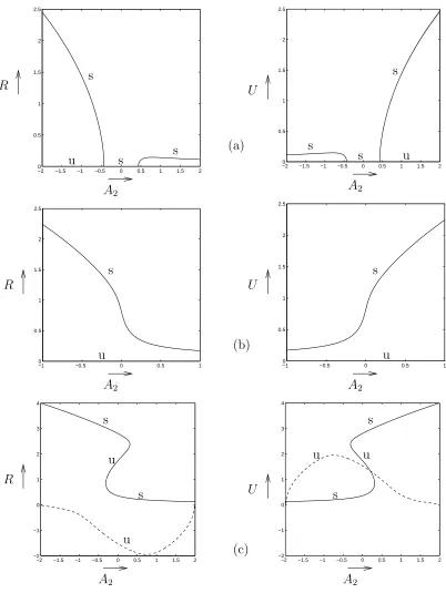
These equations are relatively straightforward to solve numerically and in figure 4 we show solutions to (29) and (30), obtained in this manner, for various values of Γ2. The solutions
plotted are not complete. In particular, since equations (29)-(30) are invariant under the transformation (R, U)→(−R,−U), solutions occur in pairs, and we plot only one of every pair. We have also ommited the zero solution (R, U) = (0,0) from some of the plots.
The reader should observe how the dependence of (R, U) on A2 changes as Γ2 increases.
For sufficiently small Γ2 (figure 4(a)) there is a region centred on A2 = 0 where the only
solution is the zero solution. Beyond Γ2 =−1/4 this region dissapears such that for all values
of A2 a non-zero solution pair exists. As Γ2 is increased still further the curves representing
the original solution pairsR =R(A2) and U =U(A2) develop a fold and, for some values of
A2, another solution pair appears. It is possible to find formulae which give the positions, in
the (Γ2, A2) plane, of (I) the boundary of the normal region in which only the zero solution
exists and (II) the fold in the solution surface. We calculate the former by linearising (29) and (30) about (R, U) = (0,0) and looking for bifurcations from the zero solution. These occur along the lines
Γ2 =−
A22+ 1 16
1/2
and Γ2 =
A22+ 1 16
1/2 .
The normal region is bounded by the first of these two lines and lying in
Γ2 <−
A22+ 1 16
−20 −1.5 −1 −0.5 0 0.5 1 1.5 2 0.5
1 1.5 2 2.5
−2 −1.5 −1 −0.5 0 0.5 1 1.5 2 0
0.5 1 1.5 2 2.5
−10 −0.5 0 0.5 1 0.5
1 1.5 2 2.5
−2 −1.5 −1 −0.5 0 0.5 1 1.5 2 −2
−1 0 1 2 3 4
−2 −1.5 −1 −0.5 0 0.5 1 1.5 2 −2
−1 0 1 2 3 4 −1 −0.5 0 0.5 1
0 0.5 1 1.5 2 2.5
U
U U A2
A2
A2 A2
A2
A2
R
R
R
(a)
(b)
(c) s
u s s
s
s
s s
s
u
s
u
u
s
u
s
s u
[image:17.595.95.497.111.646.2]u u
Figure 4: The figure shows plots of R and U versus A2 for constant values of Γ2. In (a)
−3 −2 −1 0 1 2 3 4 −2
−1 0 1 2
Normal
Winding no.=m+1
Winding no.=m A2
[image:18.595.171.406.109.287.2]Γ2
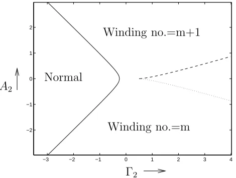
Figure 5: The phase diagram for a ring with small variations in thickness in the vicinity of a critical point.
We look for the fold in the solution surface by searching for infinities of∂η/∂A2. These occur
for values of η satisfying
sin 2η=
1 2Γ2
1/3
and cos 2η=
3A2
Γ2
1/3
. (33)
The fold thus lies along a curve in the (Γ2, A2) plane satisfying
1 2Γ2
2/3 +
3A2
Γ2
2/3
= 1. (34)
This curve is plotted, along with the boundary of the normal region, in figure 5. The dashed and dotted lines represent the fold and the solid line the boundary of the normal region.
4.3.1 Weakly nonlinear stability analysis.
We need now to investigate the stability of the large number of solutions to equation (1) that exist in the vicinity of the critical point. A linear stability analysis about the normal state reveals that all single wavenumber perturbations to the solution ψ = 0 decay exponentially in time with the exception of the m0
th and (m+ 1)0
for solutions to the time dependent model (2) and (4) of the form
ψ = δ1/2 R(τ)eims +U(τ)ei(m+1)s
+δ3/2ψ2+· · · ,
A = (m+ 1/2) +δA2+· · · ,
Γ = 1
4+δΓ2+· · · , Φ = O(δ2),
where τ is the long time variable given by τ =δt. Adopting an approach similar to that in
§4.3 above we find the following equations for R0
(τ) and U0
(τ):
dR
dτ +R 4(A2−Γ2) + (|R|
2+ 2|U|2)
= U, (35)
dU
dτ +U −4(A2+ Γ2) + (|U|
2+ 2|R|2)
= R. (36)
We can ascertain the stability of solutions to the steady problem (29) and (30) for any given (Γ2, A2) by plotting a phase diagram. Alternatively we can attempt to make a more general
statement regarding the stability of the solution manifold by linearising equations (35)-(36) about the steady solution (R, U) = (ρsinη, ρcosη)
R = ρsinη+eλτr1,
U = ρcosη+eλτu1,
where 1. Substituting the above into (35)-(36) and proceeding to O() one finds that (r1, u1)T is an eigenvector of the matrix
−(ρ2(3 sin2η+ 2 cos2η) + 4(A2−Γ2)) 1−2ρ2sin 2η
1−2ρ2sin 2η 4(A2+ Γ2)−ρ2(3 cos2η+ 2 sin2η)
with corresponding eigenvalue λ. This eigenvalue satisfies the quadratic equation
aλ2+bλ+c= 0, (37)
whose coefficients are determined in the usual manner. After considerable manipulation, in which we eliminate ρ and cos 2η by reference to equation (32), we find that these may be written in the form
a= 3 sin22η b= 2 sin22η
8Γ2+
5 sin 2η
c= 8 sin 2η
Γ2+
1 sin 2η
1−2Γ2sin32η
In order for a solution to be stable we require that both solutions to equation (37) have negative real part. Since a >0 this amounts to requiring bothb andcbe positive. Referring to equation (32b) we see that the physically relevant solutions are those for which
4Γ2+
1
sin 2η >0. (38)
For Γ2 >0 such solutions are stable (i.e b >0 and c >0) iff
0<sin 2η <
1 2Γ2
1/3 .
For Γ2 <0 all solutions which satisfy the condition (38) are stable.
Remark It is clear form equation (32a) that sin 2η= 0 is never a solution. It follow that a sheet of the solution manifold may only change from unstable to stable or vice-versa along lines on which sin 2η= (1/(2Γ2))1/3 and Γ2 >0. It is straightforward to show that solutions
of (32a) can only adopt this value of sin 2η at positions in the (Γ2, A2) plane satisfying (34)
and furthermore that cos 2η = (3A2/Γ2)1/3. Referring back to equation (33) we can see
that the switch in stability occurs along a fold in the sheet. Hence the sheet that bifur-cates from the normal solution along the line Γ2 =−(A22 + 1/16)1/2 is always stable except
where it has folded over on itself (this sheet is represented by the solid curve in figure 4). The other non-zero sheet to the solution manifold bifurcates from the zero solution along Γ2 = (A22 + 1/16)1/2 and is always unstable R and U take opposite signs along this sheet,
corresponding to negative vales of sin 2η(this sheet is represented by the dashed line in figure 4c).
We can investigate the stability of the normal solution (R, U) = (0,0) by adopting a similar approach to that taken above. We linearise equations (35)-(36) about the zero solution by substitution of
R=eλτr
1, U =eλτu1, 1.
At O() we find an eigenvalue problem for (r1, u1)T with corresponding eigenvector λ.
De-termining λ in the usual manner we find
λ= 4 Γ2±
A22+ 1 16
1/2! .
The normal solution is therefore stable only for
Γ2 <−
A22+ 1 16
Physical interpretation of the solutions. We have investigated the solution structure, and stability, of a loop with slightly non-uniform thickness in the vicinity of a critical point. We can interpret the results physically with the aid of figure 5. To the left of the solid line the only solution is ψ= 0 corresponding to the normal state. As this line is crossed the normal solution loses stability and a stable superconducting solution bifurcates. This solution has winding numberm+ 1 for A2 >0 and winding number m forA2 <0. A completely smooth
transition between winding numbers occurs if the system traverses the phase plane, from top to bottom or vice-versa, without crossing the dotted or dashed lines (see figure 4(b)). If however a transversal of the phase plane is made from bottom to top which crosses the dashed line the transition between winding number occurs suddenly; as the dashed line is crossed the winding numbermsolution loses stability and the system evolves to the winding number m+ 1 solution. The reverse transition, from winding number m+ 1 to m, occurs along the dotted line.
5
Conclusion
In this work we have investigated the bifurcations of a loop of superconducting wire between different states. For a wire of uniform thickness we found, in agreement of the results of Berger and Rubinstein [1] and Gorff and Parks [3], a supercritical bifurcation between the normal state and a superconducting state whose topological winding number is determined by the magnetic field. We also found a series of subcritical bifurcations occuring between superconducting states with different winding numbers. Investigation of the stability of these states led us to infer that the system exhibits hysteresis as a transition is made from one winding number to an adjacent one and back again. The lines representing these two different types of transition in state space (see figure 2) intersect at a series of points (the critical points).
In the latter portion of this paper we investigated the effect that small nonuniformities in the thickness of the wire loop have upon the bifurcation structure of the system. We found that a supercritical bifurcation still occurs between the normal and superconducting states; the effect of the nonuniformity is only to increase the temperature (lower Γ) at which it occurs. The transition between superconducting states of different winding numbers no longer occurs at a subcritical bifurcation, but on a fold (see figure 3). The most marked change, though, is in the vicinity of a critical point. Here variations in the thickness cause the folded region of the solution surface to separate from the normal-superconducting bifurcation. Thus in a narrow region close to this bifurcation the transition between superconducting states with different winding numbers is completely smooth.
References
[1] J. Berger and J. Rubinstein,Bifurcation analysis for phase transitions in superconduct-ing rsuperconduct-ings with nonuniform thickness, S.I.A.M. J. Appl. Math. 58, 103 (1998).
[2] V.L. Ginzburg and L.D. Landau,On the theory of superconductivity, J.E.T.P.20, 1064 (1950).
[3] R.P. Groff and R.D. Parks,Fluxoid quantisation and field induced depairing in a hollow superconducting microcylinder, Phys. Rev. 176, 568 (1968).
[4] W.A. Little and R.D. Parks, Observation of quantum periodicity in the transition tem-perature of a superconducting cylinder, Phys Rev. Lett. 9, 9 (1962).
[5] V.M. Fomin, V.R. Misko, J.T. Devreese and V.V. Moshchalkov,On the superconducting phase boundary for a mesoscopic square loop, Solid State Comm.101, 303 (1997).
[6] V.V. Moshchalkov, L. Gielen, C. Strunk, R. Jonckheere, X. Qiu, Van Haesendonck and Y. Bruynseraede, Effect of sample topology on the critical fields of mesoscopic supercon-ductors, Nature,373, 319 (1995).
[7] G. Richardson and J. Rubinstein, A one-dimensional model of superconductivity in a thin wire of slowly varying cross-section, (preprint).
[8] J. Rubinstein and M. Schatzmann,Asymptotics for thin supercondcting rings, J. Math. Pure Appl., (to appear).