Gender and gaze gesture recognition for human computer interaction

Gender and Gaze Gesture Recognition for Human-Computer Interaction

Wenhao Zhang

, Melvyn L. Smith, Lyndon N. Smith, Abdul Farooq

Centre for Machine Vision, Bristol Robotics Laboratory, University of the West of England, T Block, Frenchay Campus, Coldharbour Lane, Bristol, BS16 1QY, UK

Abstract

The identification of visual cues in facial images has been widely explored in the broad area of computer vision. However theoretical analyses are often not transformed into widespread assistive Human-Computer Interaction (HCI) systems, due to factors such as inconsistent robustness, low efficiency, large computational expense or strong dependence on complex hardware. We present a novel gender recognition algorithm, a modular eye centre localisation approach and a gaze gesture recognition method, aiming to escalate the intelligence, adaptability and interactivity of HCI systems by combining demographic data (gender) and behavioural data (gaze) to enable development of a range of real-world assistive-technology applications.

The gender recognition algorithm utilises Fisher Vectors as facial features which are encoded from low-level local features in facial images. We experimented with 4 types of low-level features: greyscale values, Local Binary Patterns (LBP), LBP histograms and Scale Invariant Feature Transform (SIFT). The corresponding Fisher Vectors were classified using a linear Support Vector Machine. The algorithm has been tested on the FERET database, the LFW database and the FRGCv2 database, yielding 97.7%, 92.5% and 96.7% accuracy respectively.

The eye centre localisation algorithm has a modular approach, following a coarse-to-fine, global-to-regional scheme and utilising isophote and gradient features. A Selective Oriented Gradient filter has been specifically designed to detect and remove strong gradients from eyebrows, eye corners and self-shadows (which sabotage most eye centre localisation methods). The trajectories of the eye centres are then defined as gaze gestures for active HCI. The eye centre localisation algorithm has been compared with 10 other state-of-the-art algorithms with similar functionality and has outperformed them in terms of accuracy while maintaining excellent real-time performance.

The above methods have been employed for development of a data recovery system that can be employed for implementation of advanced assistive technology tools. The high accuracy, reliability and real-time performance achieved for attention monitoring, gaze gesture control and recovery of demographic data, can enable the advanced human-robot interaction that is needed for developing systems that can provide assistance with everyday actions, thereby improving the quality of life for the elderly and/or disabled.

Keywords: Assistive HCI, Gender recognition, Eye centre localisation, Gaze analysis, Directed advertising

1.

Introduction

With the emergence of personal computing in the late 1970s, the concept of Human-Computer Interaction (HCI) was pushed rapidly and steadily into the environment where the individual role of science or engineering was not sufficient for addressing the urgent need for increasing the usability of computer software and operating systems [1]. The potential of

* Corresponding author.

Email Address: [email protected]

increased accessibility to personal computers and demand for higher usability [2] of computer platforms called for the practical need for HCI and a synthesis of science and engineering. As personal computers present more digital information to people, the way people perceive, process and respond to such data has largely altered. HCI has therefore not only become central to information science theoretically and professionally, but also has stepped into peoples’ lives, offering multiple types of communication channels, i.e. modalities. These modalities gain their input via various types of sensors, mimicking human sensors including visual, audio and haptic sensors [2]. They individually or combined give rise to a wide array of HCI systems. Among the various types of sensors, the visual sensor and the resulting visual based interaction modality are the most widespread, taking visual signals as inputs, which include but are not limited to images/videos of faces, bodies and hands [3]. The corresponding research spans the areas of gaze tracking, gait analysis, and recognition of face, gender, age, gesture and facial expression. While face recognition reveals an individual’s identity, gender/age recognition aims to gather human demographics for the system to understand human characteristics. Facial expression recognition further estimates human affection states and gathers emotional cues while gaze tracking serves to extract users’ attentive information and to predict their intentions.

These modalities, independent or combined, have played different assistive roles in their corresponding HCI applications. As an example of gaze tracking, smart solutions are available that monitor the gaze direction of a driver in order to identify driver distraction/drowsiness and provide timely alerts [4]. These driver assistance systems, capable of detecting and acting on driver inattentiveness, are of great value to road safety. In the area of gesture recognition, a sterile browsing tool, ‘Gestix’, has been designed for doctor-computer interaction. This assistive technology provides doctors the sterility needed in an operation room where radiology images can be browsed in a contactless manner. A doctor’s hand is tracked by a segmentation algorithm using colour model back-projection and motion cues from image frames [5]. Moreover, when expression recognition is concerned, an intelligent tutoring system, namely a Learning Companion, is proposed to predict when a learner might be frustrated, initiate interaction depending on the user’s affective state and provide support accordingly [6].

With regard to the visual modality, we categorise these tasks as ‘demographic recognition’ (e.g. age and gender recognition) or ‘behavioural recognition’ (e.g. gaze analysis), according to the source and the utilisation of visual signals. In this paper, we propose a HCI strategy by combining demographic and behavioural recognition such that more natural, interactive and user-centred HCI environments can be created. More specifically, although demographic data reveal user characteristics and help define the ‘initial state’ and the ‘general theme’ of a HCI session, they cannot address the dynamic nature of a HCI session where user behaviours are constantly changing. Therefore, on the one hand, behavioural recognition reflects user attentions and intentions; on the other hand, it allows a user to issue commands and to actively interact with a HCI system through various means. As a result, the combination of demographic and behavioural recognition provides fused knowledge throughout a HCI session and better mimics a natural face-to-face interaction.

Although research in HCI has become increasingly active and sophisticated, a few issues remain unresolved that restrict most works from being transformed into assistive HCI systems that can benefit the daily life of human beings. We summarise the three major general issues that undermine the practicability of these works as follows:

1) Lack of accuracy in real-world scenarios. Many research works are tested on controlled databases where ideal illuminations, high-resolution images and desirable viewpoint are available. When tested under various types of scenes with dynamic environmental factors, their performance will drop severely.

3) High dependence on expensive or inconvenient hardware configuration. The cost and the complexity of algorithm implementation will limit the usability and applicability of any method. Cheap yet effective methods are in high demand in order to boost assistive technologies.

In order to fill these gaps, in section 3, we present an accurate gender recognition method that exhibits high accuracy and robustness under controlled and uncontrolled environments. This method puts Fisher Vectors at its core and encodes low-level local features (e.g. greyscale values, Local Binary Pattern (LBP), LBP histograms and the Scale Invariant Feature Transform (SIFT)) into more discriminative features for gender classification. State-of-the-art accuracy is achieved by only a linear Support Vector Machine (SVM), which further confirms the superiority of Fisher Vectors.

In section 4, we propose a modular eye centre localisation method that makes use of isophote and gradient features extracted by its two modules. The first module performs an initial estimation of eye centre locations using isophote features from face images and filters eye centre candidates for the second module. The second module then updates the eye centre locations using only local gradient features. This coarse-to-fine and global-to-regional scheme ensures that this method is fast and accurate.

To further explore the localised eye centres, in section 5, we introduce gaze gesture recognition, i.e. classification of the trajectory patterns of eye centre locations in consecutive frames. These gaze gestures provide contactless substitutes for mouse/keyboard input. Gaze gesture recognition therefore offers great assistance to the elderly and the disabled in accessing a variety of digital systems.

As our algorithms only require a standard webcam to capture image data, we implemented all the above mentioned algorithms and integrated them in a directed advertising system – which is one of the assistive technology tools our algorithms can bring to real-world applications. The directed advertising system combines the interpretation of demographic data (gender) and behavioural data (gaze) in order to deliver customised advertisements to its users and allow them to remotely browse advertising messages.

In summary, the main contribution of this paper is fourfold.

1) A novel gender recognition method utilising the Fisher Vector encoding method – a generic method that can encode almost all types of features but still maintains low complexity in implementation. It also proves to have high accuracy and robustness against head poses. To the best of our knowledge, this is the first time that Fisher Vectors have been employed for gender recognition.

2) A modular eye centre localisation method consisting of two modules and a Selective Oriented Gradient (SOG) filter. The eye centre localisation method has proved to be accurate, fast and, more importantly, robust to in-plane and out-of-plane head rotations. The SOG filter is specifically designed to detect and remove strong gradients from eyebrows, eye corners and self-shadows that many other methods suffer. The SOG filter also resolves general tasks regarding the detection of curved shapes.

3) Design of gaze gestures and a gaze gesture recognition algorithm. The algorithm captures the relative attention of the users and enables them to control HCI systems by issuing gaze gestures. This will largely enhance the interactivity of current HCI systems.

(including the elderly and the disabled), with accessing HCI systems with ease and convenience, in a wide range of applications.

2.

Related work

A number of assistive technologies that utilise vision modalities have been introduced in the preceding section. In this section, we explore the combination of gender recognition and eye/gaze analysis and review a number of related state-of-the-art methods. We provide a summary of the current research state for gender recognition, eye centre localisation and gaze/gaze gesture analysis; and we discuss their potential benefits for assistive HCI applications, and identify the limitations that will critically hinder advancement in this area.

2.1. Gender recognition

Gender recognition from facial images, i.e. gender classification, is a challenging task in that a face exhibits a wide range of intra-class variations due to facial attributes or environmental factors. The former complications mainly include age, ethnicity and makeup while the latter include illumination condition, head pose, facial occlusion and camera quality.

Most high-performance gender recognition methods involve machine learning and follow four stages: face detection, facial image pre-processing, feature extraction and classification [7].

For the face detection stage, the Viola-Jones face detector [8] has been widely adopted due to its ease of implementation and relatively high accuracy. It is essentially a face detector that employs Haar-like features, a classifier learning with AdaBoost and a cascade structure [9]. It can operate in real time and has allowed many practical applications to boom in the last decade.

For the image pre-processing stage, normalisation, i.e. contrast and brightness adjustment; image resizing and face alignment are commonly considered useful despite their varied implementation details. Among them, face alignment has been reported to be able to guarantee an increase in the classification accuracy by a number of studies. For example, in a research [10] evaluating a number of gender classification methods, it is concluded that Support Vector Machine (SVM) outperformed other classification methods with 86.54% accuracy on 36×36 aligned images, and that higher accuracy could be achieved by improving the implementation of the automatic alignment methods. Another research [11] with regard to gender classification illustrated that face alignment brought an increase to the classification accuracy for various methods including use of neural networks, SVM, and Adaboost. Different pre-processing methods are experimented with in our method with the results reported in section 3.

For the feature extraction and selection stage, a wide range of features are experimented with and evaluated in the literature. They include intensity values from greyscale images [12], LBP [13,14], facial strips [15], Haar-like features [9], SIFT features [16], etc. These features can be extracted globally from complete face images or locally from defined sub-regions of the face images.

For the classification stage, SVMs and neural networks have been the most popular classifiers. SVMs with different kernels were investigated in [12] and convolutional neural networks were adopted by [17] and [18] as gender classifiers.

A decision-fusion based method is presented by [19] that utilises multiple SVMs to classify intensity values, local binary patterns and histogram of edge directions as features. The three types of features are extracted from images of various sizes. Finally all classification results are integrated to make the final decision by means of majority voting, leading to 99.07% accuracy. However this result is obtained from a small subset of the FERET database and their validation method is not sophisticated enough to reflect the performance of their approach objectively. In addition, only controlled databases are used for training and testing in this research so that the applicability of this approach to dynamic environments remains unevaluated. Similarly, another study [15] employs 10 regression functions to conduct region-based classifications and feed the vector of classification results into an SVM to generate the final decision. Despite the 98.8% accuracy with the FERET database they reported, they didn’t illustrate their evaluation method and the split of training and testing data. The reappearance of the same subject in both the training and testing data may account for the high accuracy they obtained. A face alignment scheme is compulsory to their approach, the absence of which leads to a 6% drop in the classification rate, bringing 98.8% down to 92.8%. This is an inherent limitation of conventional region-based approaches where defined facial regions have to be perfectly aligned. A fusion-based method [20] proposed to integrate different facial regions for gender recognition using the ‘matcher weighing fusion’ method. The facial landmarks for segmenting the face into its sub-regions are detected by a profile-based method and a curvature based method. Interestingly they prove experimentally that the fusion of multiple facial sub-regions is superior to the complete face region alone and that the upper face contains more discrimination ability regarding gender classification. Apart from classification fusion, feature fusion provides an alternative way to boost gender classification rates. In [21], two types of appearance features, i.e. the LBP features and the shape index features, were fused to characterise facial textures and shapes. The resulting classification rate on the FRGCv2 dataset was up to 93.7%.

With individual works reviewed, we draw conclusions from the literature regarding the preferences in gender classification. 1) SVM and neural networks are the most popular classifiers. 2) LBP and its variations are the most popular features. 3) Most studies use the FERET database as the standard evaluation database. 4) Most works are carried out under a well-controlled environment while real-world implementation and evaluation lack exploitation. 5) Most works incorporate face alignment in the pre-processing stage. 6) Most works employ the 5-fold cross validation for accuracy estimation.

In most gender classification studies, limitations and complications are seen as both intrinsic factors and extrinsic factors. The former type is mainly the consequence of large amount of variation in facial appearance due to aging, makeup, facial occlusion, ethnicity and accessories. The latter type is largely due to environmental variations such as camera viewpoint (head pose), illumination condition, etc. Variations incurred by undesirable illumination conditions in particular are difficult to address by employment of powerful classifiers, but rather should be tackled by seeking for more robust and reliable facial features. This has defined the trend for gender recognition researches – the exploitation of 3D features that are independent of lighting conditions. 3D features have been employed individually [20, 22] or fused [21, 23] with 2D features to better characterise face shapes and textures. This will be reflected in our future works aiming to extend the proposed gender recognition algorithm by incorporating 3D features.

2.2. Eye/gaze analysis

According to the features extracted, eye centre localisation methods fall into two main categories: inherent feature based methods and additive feature based methods. An additive feature based method actively projects infrared illumination toward the eyes that result in reflections on the corneas, which are referred to as ‘glints’ in the literature [24]. Being highly reliant on dedicated devices, this method essentially alters the primary task of eye centre detection into corneal reflection detection as a simplified detection task. A passive inherent feature based method is more generalizable since it employs characteristic features from the eye region itself and therefore becomes the method we explore in this paper. It can be further divided into 1) eye geometry or morphology based methods that utilise gradient, isophote or curvature features to estimate the eye centre that comply with geometrical or morphological constraints, 2) model and machine learning based methods where distinct features are extracted to train a model to search for the eye region that best matches the model representation, and 3) hybrid methods which normally follow a multi-stage scheme that comprises the previously summarised. While several methods have achieved interesting results, they have also exhibited their respective limitations.

One geometrical feature based method [25] localises eye centres by means of gradients. In this approach, the iris centre obtains the maximised value in the objective function that peaks at the centre of a circular object. Its performance declines in the presence of strong gradients from eyelids, eyebrows, shadows and occluded pupils that overshadow iris contours. Another unsupervised method employing geometrical features that was investigated is Self-Similarity Space. Here image regions that can maintain peculiar characteristics under geometric transformations receive high self-similarity scores [26].

Regarding model and machine learning based methods, for all algorithms that utilise extracted features to train a model, it holds that the training data are of critical influence on the performance of the algorithms [27]. More specifically, variations posed by illumination and head rotation have a huge impact on the accuracy and robustness of the algorithm for most types of features. Inspired by Fisher Linear Discriminant (FLD) [28], [29] designed a linear filter trained by the image patches extracted from normalized face images. This method not only considers the high response from the filtered image, but also examines a rectangular neighbourhood around the estimated eye centre positions. This is based on the observation that a pupil in an image is formed by a collection of dark pixels within a small region. Another machine learning based method [30] focuses on the design of a novel classifier rather than the extraction of representative features. This method introduces a 2D cascade AdaBoost classifier that combines bootstrapping positive samples and bootstrapping negative samples [9]. The final localisation of an eye can be achieved either by weighting all classifier results for high precision or by cascading all classifiers (i.e. only adopting the result from the first classifier that detects an eye window) for increased efficiency. In addition, a number of studies are only effective for frontal faces. For example, [31] employed a cumulative distributed function (CDF) for adaptive centre of pupil detection on frontal face images. Their approach firstly extracts the top-left and top-right quarters of a face image as the regions of interest and then filters each region of interest with a CDF. An absolute threshold is defined for the filtering process given the fact that the pixels in the pupil region are darker than the rest of the eye region. Another study on frontal faces [32] explored edge projections for eye localisation. With a face image available, their method firstly defines a rough horizontal position for the eye region according to facial anthropometric relations. After the eye band is cropped, it gathers eye candidate points that are extracted by a high-pass filter of a wavelet transform. A Support Vector Machine (SVM) based classifier [33] is then used to estimate the probability value for every eye candidate. This type of method normally requires that all face images are perfectly aligned so that the facial geometry agrees with facial anthropometric relations as the prior knowledge.

rather than absolute eye fixation points. Calibration is also unnecessary and this therefore makes eye gesture more suitable for real-world applications. The two interaction methods are further compared by [35] which suggested that “gaze gestures are not only a feasible means of issuing commands in the course of game play, but they also exhibited performance that was at least as good as or better than dwell selections”. Another study [36] achieved gaze gesture recognition for HCI under more general circumstances. It employs the hierarchical temporal memory pattern recognition algorithm to recognise predefined gaze gesture patterns. 98% accuracy is achieved for 10 different intentional gaze gesture patterns. Some other works on gaze gestures dedicated to HCI have similar limitations. Firstly, they all depend on active NIR lighting for eye centre localisation. Secondly, the eye centre localisation algorithms work at only relatively short distance.

3.

Fisher Vector for Gender recognition

As seen from the literature, most methods regarding gender recognition and gaze analysis lack robustness and suffer from various limitations in real-world scenarios. To bridge these gaps, we explore novel methods that can assist HCI implementations robustly and efficiently while maintaining high accuracy. In this section, we introduce a gender recognition method that utilises Fisher Vectors as discriminative features.

3.1. Fisher Vector principle

A Fisher Vector (FV) is an encoded vector that applies Fisher kernels on visual vocabularies where the visual words are represented by means of a Gaussian Mixture Model (GMM). The Fisher kernel function is derived from a generative probability model, and provides a generic mechanism that combines the advantages of generative and discriminative approaches.

As a core component of a FV, a GMM is a parametric probability density function represented as a weighted sum of Gaussian component densities as given by equation (1) [37]

𝑝(𝒙|𝜆) = ∑ 𝜔𝑖 𝒩(𝒙|𝝁𝒊, 𝝈𝒊) 𝐵

𝑖=1

(1)

where 𝒙 is a 𝐿-dimensional data vector, 𝜆 = {𝜔𝑖, 𝝁𝒊, 𝝈𝒊, 𝑖 = 1,2, … , 𝐵} is the collective representation of the GMM

parameters – 𝜔𝑖 the mixture weights, 𝝁𝒊 the mean vector and 𝝈𝒊 the covariance matrix. 𝐵 is the number of Gaussians. The

component 𝒩(𝒙|𝝁𝒊, 𝝈𝒊) is further described in equation (2).

𝒩(𝒙|𝝁𝒊, 𝝈𝒊) =

𝑒{−12(𝒙−𝝁𝒊)′𝝈𝒊−𝟏(𝒙−𝝁𝒊)}

(2𝜋)𝐿/2_|𝝈

𝒊|1/2 (2)

The mixture weights are subject to the constraint in equation (3).

∑ 𝜔𝑖 𝐵

1

= 1 (3)

The covariance matrices are assumed to be diagonal since any distribution can be decomposed into a number of weighted Gaussians with diagonal covariances.

Let 𝑿 = {𝒙𝒕, 𝑡 = 1,2, … , 𝑇} be the set of descriptors of low-level features extracted from an image, and it is assumed that

log 𝑝(𝑿|𝜆) = ∑ log 𝑝(𝒙𝒕|𝜆) 𝑇

1

(4)

The descriptors 𝑿 can be described by the gradient vector:

𝜓𝜆𝑿=

∇𝜆 𝑙𝑜𝑔𝑝(𝑿|𝜆)

𝑇 (5)

A natural kernel on these gradients is:

𝜘(𝑿, 𝒀) = 𝜓𝜆𝑿′ ℱ𝜆−1 𝜓𝜆𝒀 (6)

where ℱ𝜆= ℒ𝜆′ℒ𝜆is the Fisher information matrix and Ψ𝜆𝑿= ℒ𝜆 𝜓𝜆𝑿 is referred to as the Fisher Vector of 𝑿.

Let 𝛾𝑡(𝑖) denotes the soft assignment of descriptor 𝒙𝒕 to the Gaussian component 𝑖:

𝛾𝑡(𝑖) = 𝑝(𝑖|𝒙𝒕, 𝜆) =

𝜔𝑖𝒩(𝒙𝒕|𝝁𝒊, 𝝈𝒊)

∑𝐵𝑗=1𝜔𝑗𝒩(𝒙𝒕|𝝁𝒋, 𝝈𝒋)

(7)

The gradients of Gaussian component 𝑖 with respect to the mean 𝝁𝒊and the covariance 𝝈𝒊 respectively are:

Ψ𝜇,𝑖𝑿 =

1 𝑇√𝜔𝑖

∑ 𝛾𝑡(𝑖) 𝑇

1

(𝒙𝒕− 𝝁𝒊

𝝈𝒊 ) (8)

Ψ𝜎,𝑖𝑿 =

1 𝑇√2𝜔𝑖

∑ 𝛾𝑡(𝑖) 𝑇

1

[(𝒙𝒕− 𝝁𝒊)

𝟐

𝝈𝒊𝟐 − 1] (9)

Finally a FV is represented as:

Φ = {Ψ𝜇,1𝑿 , Ψ𝜎,1𝑿 , … , Ψ𝜇,𝑁𝑿 , Ψ𝜎,𝑁𝑿 } (10)

Therefore, when images from a certain database produce a large number of feature descriptors, a GMM can be trained by them using the Maximum Likelihood (ML) estimation. The difference between every individual descriptor and every Gaussian distribution is captured by equation (8) and (9), which is further stacked into a FV by equation (10). Following this manner, a FV can be computed for every descriptor, which encodes the difference between a single descriptor and all descriptors described by the GMM. This means that the difference between an image and the entire training dataset is preserved. As a result, a FV is provided with contextual definition and enhanced saliency for classification.

3.2. Fisher Vector encoding for gender recognition

Fisher Vectors have been used for face recognition and have proved to be an excellent encoding method [38]. The FV encoding approach consists of 5 main stages: 1) face pre-processing, 2) low-level feature and face descriptor computation, 3) dimensionality reduction/feature selection, 4) FV encoding and 5) classifier training. In more detail, we illustrate the 5 primary stages adopted by our method as follows.

1) Face pre-processing.

managed by excluding the background margins from the width by a ratio of 𝑟𝑤 and expanding the length by a ratio of 𝑟𝑙. Let the side of a square region detected by the face detector be 𝑓𝑠, the length of a reshaped face region be 𝑓𝑙 and the width be 𝑓𝑤. A reshaped face region can be defined as:

{ 𝑓𝑤 = 𝑓𝑠 × (1 − 𝑟𝑤)

𝑓𝑙 = 𝑓𝑤 × (1 + 𝑟𝑙) (11)

where 𝑟𝑤 = 0.12 and 𝑟𝑙 = 0.33 in our experiments. This ensures that the reshaped face region has a uniform aspect ratio (i.e. 3:4), while keeping its size relative to that originally detected by the face detector. Facial regions were further resized to the same size in the next step with or without histogram equalisation. Face alignment was also experimented with and its impact was investigated.

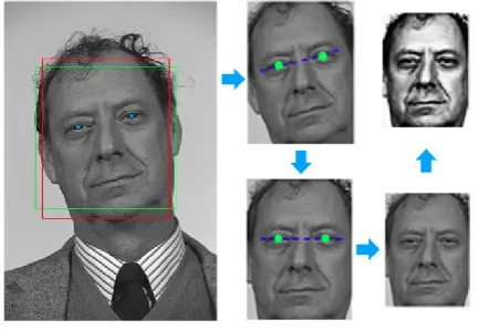
An optional step at this stage is face alignment, which is intended to compensate for different head poses that are likely to sabotage most gender recognition algorithms. To evaluate the robustness of our method against different head poses, we conducted experiments (see Section 3.3) with or without face alignments. Eye centre coordinates obtained by the proposed eye centre localisation method (introduced in Section 4) were employed as facial landmarks for the alignment. However, eye centres accurately localised by other methods or other types of facial landmarks (e.g. eye corners and nose tip) should also suffice to perform the alignment. Fig. 1 further illustrates the face pre-processing stage with an example.

Fig. 1. An illustration of face pre-processing, including face detection, face alignment (optional), and histogram equalisation (optional). The two boxes in solid lines around the face area represent the detected facial region (square) and the reshaped facial region (rectangular), respectively.

Fig. 2. Geometry of patch-based dense feature descriptors

2) Low-level feature and face descriptor computation.

Conventionally, one face image produces only one feature vector, namely a descriptor (e.g. the LBP features) or a few descriptors around keypoints (e.g. the SIFT features). In both cases, feature descriptors are sparsely extracted. Different from both methods, we extract dense descriptors at every pixel location. Firstly, we segment a face image into a number of overlapping patches of the same size. Specifically, these patches are obtained by sliding a 𝑟 × 𝑟 window across an image horizontally and vertically with a predefined stride 𝑠 (𝑠 ∈ ℤ). One descriptor per patch rather than one descriptor per image is calculated. The geometry of the patch-based descriptors is shown in Fig. 2. For example, vector (𝑝𝑥𝑐, 𝑝𝑦𝑐) records the

centre position of the 𝑎𝑡ℎ _{(𝑎 ∈ ℕ, 𝑎 ≤ 𝑝𝑛) patch in the image. The centre position of the first patch is therefore (𝑟/2, 𝑟/2).}

𝑝𝑛 = 𝑚 − 𝑟 + 1

𝑠 ×

𝑛 − 𝑟 + 1 𝑠 ,

𝑟 < min(𝑚, 𝑛)

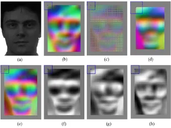
1 ≤ 𝑠 ≤ min(𝑚, 𝑛) (12)

Although a number of pixels at the margins of an image cannot be the centres of a sliding window, they are incorporated by at least one image patch and are therefore involved in the formation of image descriptors. Low-level dense features can be visualised by mapping the top three principal components to the RGB space. A similar process can be found in [39]. As an example, dense SIFT features extracted with different parameters can be seen in Fig. 3.

Fig. 3. Dense SIFT feature visualisation in the RGB colour space. The square on the top left corner denotes the size and centre of the first descriptor patch. (a) The original facial image. (b) Visualisation for r = 24 and s = 1, with histogram equalisation and root SIFT applied. (c) Visualisation for r = 24 and s = 2. (d) Visualisation for r = 36 and s = 1. (e) Visualisation for r = 24, s = 1. (f) Visualisation of the first principal component for r = 24, s = 1. (g) Visualisation of the second principal component for r = 24, s = 1. (h) Visualisation of the third principal component for r = 24, s = 1.

The visualisation implies that facial structures can be captured by densely sampled local features. It should be noted that this visualisation only reflects the top 3 principal components of the SIFT vectors which originally had 128 dimensions. Visualisation of low-level dense features under a particular colour space is only a feature-to-colour mapping process and therefore has no impact on the actual feature used for gender recognition.

3) Dimension reduction and feature selection

As one image produces multiple descriptors, linearly increasing the total number of observations as opposed to conventional methods, dimension reduction is essential in that it cuts down memory consumption and that it potentially compresses raw features into more discriminative representations.

other 64 features. As a result, although spatial information is embedded into feature vectors, the overall features are still relatively independent of global facial geometry and are therefore robust to head pose variation.

4) FV encoding

The aggregate of all descriptors from training images trains a GMM and yields model parameters which, according to equation (8) – (10), lead to FVs as encoded features. In the experiments, we utilised a publicly available toolbox [40] for GMM training and SIFT feature extraction. Among GMM parameters, different numbers of Gaussian components were experimented with, amongst which 512 was deemed a suitable value (see results in subsection 3.3 for more details). It can be calculated from equation (10) that the dimension of a FV is 2 × 𝐵 × 𝐿 = 2 × 512 × 66 = 67584. In this stage, decomposed patches are reunited to characterise a complete image, in the form of derivatives of all Gaussian components. In the computation of FVs, ℓ2 normalisation and power normalisation are applied to the vectors since they were reported to

improve classification performance [41].

5) Classifier training

Our algorithm learns a SVM classifier from all training FVs. In our experiments (see Section 3.3), a linear SVM and a SVM with a Radial Basis Function (RBF) kernel were both tested. By comparing their respective classification rate, we show that the FV encoding method only requires a linear SVM to function accurately and robustly. The employment of a SVM classifier has a twofold purpose. Firstly, it naturally fulfils the classification task by defining a hyper-plane, with or without a kernel. Its output gives the predicted labels for all testing images. Secondly, when a linear SVM is concerned, it reveals the discriminative power of each variable/feature in FVs. From the perspective of a SVM classifier, a SVM learns a hyper-plane that separates two classes with maximum margin. As the hyper-plane is defined by a decision hyper-plane normal vector 𝒘⃗⃗⃗ that is perpendicular to the hyper-plane, as well as an intercept term 𝑏, the absolute values of the elements in 𝒘⃗⃗⃗ imply the significance of the corresponding elements in the FVs. From the perspective of metric learning, the diagonal linear transformation matrix 𝑾 to be learnt has its diagonal values as in 𝒘⃗⃗⃗ . It can be considered as projecting the original data so that they are located on each side of a fixed hyper-plane, different from the former perspective where the data are fixed and the hyper-plane is unknown [42]. Both methods state that 𝒘⃗⃗⃗ , also known as the weight vector, reflects the discriminative power of individual features.

From the manner in which a FV is constructed (equation (10)), a mapping can be obtained between the features and the Gaussian components. Therefore the relationship between the discriminative power and each Gaussian component can be established. When visualised with regard to its spatial location, a Gaussian component can be used to signify the discriminability of a corresponding facial region.

3.3. Gender classification experiments and results

In order to evaluate the performance of our gender recognition algorithm under controlled environments and real-world conditions respectively, the Grey FERET database [43] (referred to as the FERET database in the rest of the paper), the Labelled Face in the Wild (LFW) database [44] and the FRGCv2 database [45] are employed.

13233 colour facial images of 5749 subjects collected from the web include all types of variation and interference (illumination, head poses, occlusion, image blur, chromatic distortion, etc.), and come in inconsistent image quality. Only one image per subject (the first image) was used in the experiment so that the same subject could not appear in both the training set and the testing set. The FRGCv2 database includes 4007 depth images belonging to 466 subjects. These data also include different ethnicities and age groups. Some sample images from the three databases are shown in Fig. 4.

Fig. 4. Sample images from (a) the FERET database 𝑓𝑎 partition (greyscale), (b) the LFW database (converted to greyscale) and (c) the FRGCv2 database (depth).

The 5-fold cross validation technique was adopted for evaluation. More specifically, the database was partitioned into 5 splits of similar size, 4 of which were used for training in each repetition with the remaining 1 split for testing. After 5 repetitions, the average classification rate was calculated as the final result.

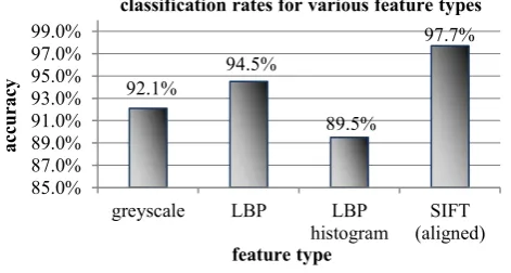
In the first group of experiments, different types of features are explored including the greyscale values, the SIFT features, the LBP features (extracted using the circularly symmetric neighbour sets [46] with 8 neighbouring pixels and radius of 1), and LBP histogram with uniform pattern. Evaluated on the FERET database, their respective performances are summarised in Fig. 5.

Fig. 5. Gender classification rates for various feature types, tested on the FERET database.

The size of facial images is 160 × 120, the sampling stride is 4 pixels, the window size for local patches is 24 × 24 and the number of Gaussian components in the GMM is 512. The classification results suggest that dense SIFT features perform the best. Therefore this feature type was selected for a further inspection regarding a number of parameters. Note that our dense SIFT features were only extracted at one scale since we did not observe higher accuracy when multiple scales were

92.1%

94.5%

89.5%

97.7%

85.0% 87.0% 89.0% 91.0% 93.0% 95.0% 97.0% 99.0%

greyscale LBP LBP

histogram (aligned)SIFT

ac

cu

ra

cy

feature type

used. In addition, we only employed a linear SVM since the RBF kernel in the experiments did not contribute to higher classification rate.

(a) (b)

(c) (d)

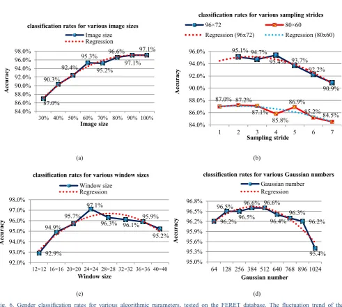
Fig. 6. Gender classification rates for various algorithmic parameters, tested on the FERET database. The fluctuation trend of the classification accuracy in each subfigure is described by a quadratic polynomial regression fit, represented by the dotted line. (a) Gender classification rates for various image sizes. (b) Gender classification rates for various sampling strides. (c) Gender classification rates for various window sizes. (d) Classification rates for various Gaussian numbers.

In the second group of experiments, parameters inspected concerned image size, size of the sliding window, sampling stride and Gaussian number. One of these parameters was altered at a time while the others remained fixed as in the last group of experiments (if not otherwise specified). Misaligned and non-normalised face images were used in this group of experiments.

1) Image size

The maximum size of selected face regions from the FERET database is 160 × 120. With the aspect ratio fixed, each face region was resized to between 30% and 90% of the maximum size, with an interval of 10%. Fig. 6(a) reflects the declined performance as the size decreases. The results suggest that larger images produce higher classification rates. This coincides with the intuition that more details reside in larger images which should generate more effective features for classification.

2) Sampling stride for local patches

87.0% 90.3%

92.4% 95.3%

95.2%

96.6% 97.1% 97.1% 84.0% 86.0% 88.0% 90.0% 92.0% 94.0% 96.0% 98.0%

30% 40% 50% 60% 70% 80% 90% 100%

Ac

cu

ra

cy

Image size

classification rates for various image sizes Image size

Regression

95.1% 94.7%

95.4% 93.7% 92.2%

90.9% 87.0% 87.2%

87.1% 85.8%

86.9%

85.2% _84.5%

84.0% 86.0% 88.0% 90.0% 92.0% 94.0% 96.0%

1 2 3 4 5 6 7

Ac

cu

ra

cy

Sampling stride

classification rates for various sampling strides

96×72 80×60

Regression (96x72) Regression (80x60)

92.9% 94.9%

95.7% 97.1%

96.3% 96.1% 95.9% 95.2% 92.0% 93.0% 94.0% 95.0% 96.0% 97.0% 98.0%

12×12 16×16 20×20 24×24 28×28 32×32 36×36 40×40

Ac

cu

ra

cy

Window size

classification rates for various window sizes Window size

Regression

96.2% 96.5%

96.5%

96.6% 96.6%

96.4% 96.3% 96.2% 95.4% 95.0% 95.3% 95.6% 95.9% 96.2% 96.5% 96.8%

64 128 256 384 512 640 768 896 1024

Ac

cu

ra

cy

Gaussian number

classification rates for various Gaussian numbers Gaussian number

Increasing the sampling stride in extracting local descriptors is comparable to decreasing the sampling rate in sub-sampling an image. Fig. 6(b) summarises the impact of sub-sampling stride. To avoid high memory usage, we firstly employed all the facial images resized to 96 × 72. Strides from 2 to 7 were experimented with in this setting. We then employed the first 500 male and female images (1000 in total) and further resized them to 80 × 60, in order that experiments with stride of 1 could be conducted. It can be seen from Fig. 6(b) that although a smaller stride tends to produces a higher classification rate in general, it will only have a dramatic influence when it goes beyond 4 pixels. Therefore, a stride of 3 or 4 can be deemed an appropriate value without incurring high memory usage at the training stage.

3) Window size of local patches

Our algorithm is appearance-based and densely extracts descriptors at local level. Broadly speaking, a larger window implicitly maintains more global and geometric information. An extreme case concerns a window as large as the entire image which removes the advantage of using local features. Hence there is a critical need for the window to be defined with an appropriate size that allows sufficient tolerance to global variations. The window size ranged from 12 × 12 to 40 × 40 pixels in the experiments, with an interval of 4 pixels. The respective classification rate is summarised in Fig. 6(c). It can be concluded that a window 15% to 20% the size of the entire image is optimal.

4) GMM component number

Fitting a generative model, the GMM, to the features is a key step in this method. Fig. 6(d) shows that the classification rate fluctuates as the number of Gaussians changes. The size of the facial images used was 128 × 96 (80% of the maximum size). The result agrees with the statement [47] that an appropriate number of Gaussian components is needed since too many components result in very few ‘per Gaussian’ statistics that are pooled together, i.e. sparse Gaussian representation. Too few Gaussians, on the other hand, are not sufficient enough to capture the uniqueness and reflect the separability of local descriptors.

5) Face alignment, histogram equalisation and root SIFT

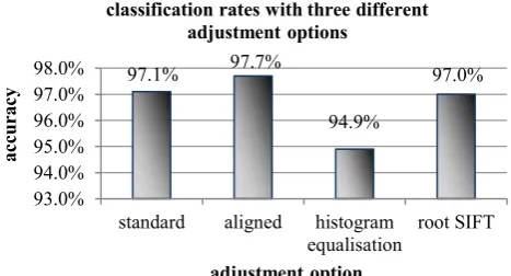
Face alignment has been reported in the literature to have a substantial impact on classification rates. Without alignment, one may experience a drop in classification rates as much as 6% [15]. In addition, applying histogram equalisation is a common pre-processing procedure that may increase classification rate. When the SIFT features are concerned, a variation of the SIFT, the root SIFT is recommended by [48], which uses the Hellinger kernel instead of the standard Euclidean distance to measure the similarity between SIFT descriptors. The impacts of the three factors were explored in this experiment, summarised in Fig. 7.

Fig. 7. Gender classification rates with or without face alignment, histogram equalisation and root SIFT implementation, tested on the FERET database

97.1% 97.7%

94.9%

97.0%

93.0% 94.0% 95.0% 96.0% 97.0% 98.0%

standard aligned histogram

equalisation root SIFT

ac

cu

ra

cy

adjustment option classification rates with three different

It should be noted that each time only one type of adjustment was made so that their impacts could be evaluated independently from other factors. As seen from Fig. 7, only face alignment plays a positive role while the other two types of adjustment decrease the classification rate. It can be claimed that the proposed algorithm is relatively robust against misalignment which caused only a 0.6% drop in the classification rate. In addition, the impact of PCA was also explored by reducing the original facial descriptors to dimensionality of 32, 64 and 96, respectively. When the first 64 principal components are employed, the highest classification rate (97.7%) can be achieved, in comparison to 96.4%, 97.2% and 95.7% for 32, 96 and 128 principal components, respectively.

As SIFT features yielded the highest classification accuracy, it was further tested on the LFW database (real data) and the FRGCv2 database (3D data). The optimal parameters identified by the previous experiments were employed in an attempt to achieve the highest classification result, except that the facial images were resized to 112 × 84 for the LFW database and 240 × 180 for the FRGCv2 database. The classification rates for aligned and misaligned images in the LFW database are 92.5% and 92.3%, respectively; the classification rate for misaligned images in the FRGCv2 database is 96.7%.

The endeavour to align faces in the LFW database sees very limited benefit (0.2% increase) and is therefore not worthwhile, since in this case and in general cases, it incurs large amount of computation. The reason behind the reduced improvement brought by face alignment on this database, compared to the 0.6% increase on the FERET database, is possibly the large extent of out-of-plane head rotation that cannot be compensated by conventional alignment algorithms.

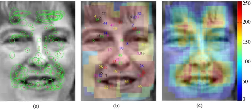
It is stated in subsection 3.2 that during the FV encoding process, spatial information of every image patch is implicitly embedded in a GMM. Therefore it is possible to restore the spatial coordinates from the Gaussian means (where the last two variables stand for the 𝑥 and 𝑦 coordinates). Similarly, the spatial variances can be restored from the Gaussian covariances, which indicate how well the spatial coordinates can represent individual patch locations. By visualising the Gaussians that correspond to the most discriminative image patches, it is possible to localise the facial regions that are most powerful in distinguishing male and female faces. Visualisation of facial discriminability is shown in Fig. 8. Note that the face image displayed is only a generic representation of facial geometry and therefore is not gender-specific.

Fig. 8. Visualisation of facial discriminability with regard to gender classification. (a) The top 128 Gaussians. (b) Facial patches at top 50 Gaussian locations. (c) The energy map for facial discriminability.

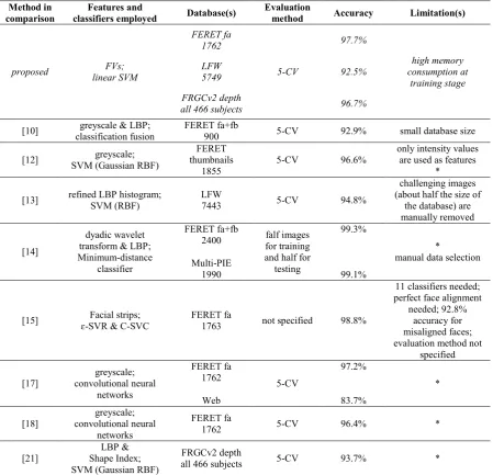
most discriminative ones. One simple solution is to construct an energy map for all pixel locations, stacking up all the patches in the previous format. The energy map agrees with the following two rules: 1) image patches with higher rankings hold more energy; 2) A pixel location where overlap exists draws energy from all the patches that cause this overlap. It can be seen that the mouth region (where male adults may have beard and moustache), the nasolabial furrows and the forehead region (where females are more likely to have bangs) are the most discriminative. This result provides insight into region-based facial discriminability so that future research on gender recognition can better target on facial regions with high discriminative power. To further validate our method, we compare the accuracy of our method to 8 other state-of-the-art methods with an evaluation of their respective limitations, detailed in Table 1.

Table 1: Comparison of the proposed method to 8 other state-of-the-art methods. The * notation indicates that training images and testing images may contain the same subjects.

Method in comparison

Features and

classifiers employed Database(s)

Evaluation

method Accuracy Limitation(s)

proposed _{linear SVM} FVs;

FERET fa 1762 5-CV 97.7% high memory consumption at training stage LFW

5749 92.5%

FRGCv2 depth

all 466 subjects 96.7%

[10] _{classification fusion} greyscale & LBP; FERET fa+fb ₉₀₀ 5-CV 92.9% small database size

[12] _{SVM (Gaussian RBF)} greyscale;

FERET thumbnails

1855 5-CV 96.6%

only intensity values are used as features

*

[13] refined LBP histogram; _{SVM (RBF)} LFW ₇₄₄₃ 5-CV 94.8%

challenging images (about half the size of

the database) are manually removed

[14]

dyadic wavelet transform & LBP; Minimum-distance classifier FERET fa+fb 2400 Multi-PIE 1990 falf images for training and half for

testing

99.3%

99.1%

*

manual data selection

[15] _{ɛ-SVR & C-SVC} Facial strips; FERET fa ₁₇₆₃ not specified 98.8%

11 classifiers needed; perfect face alignment

needed; 92.8% accuracy for misaligned faces; evaluation method not

specified

[17] convolutional neural greyscale; networks FERET fa 1762 Web 5-CV 97.2% 83.7% * [18] greyscale; convolutional neural networks FERET fa

1762 5-CV 96.4% *

[21]

LBP & Shape Index; SVM (Gaussian RBF)

FRGCv2 depth

all 466 subjects 5-CV 93.7% *

and easier to classify. It can be therefore concluded that the accuracy of the proposed gender classificaiton algorithm is among one of the highest in the literature, tested on both controlled and uncontrolled databases. The high accuracy of gender classification brought by our study allows a HCI system to understand human charactersitics. As a result, assistive systems are enabled to create user-centred HCI environments that bring more comfort and naturalness to users. In addition, the high robustness and efficiency ensure that it is applicable to practical applications rather than being limited to theoretical studies.

4.

Eye centre localisation – a modular approach

While our gender recognition method accurately and robustly gathers demographic data such that assistive HCI systems can better understand human characteristics, a hybrid method is further proposed that can perform accurate and efficient localisation of eye centres in low-resolution images and videos in real time. Therefore demographic data from gender recognition and behavioural data from eye/gaze analysis can be fused by assistive technologies in order to gain higher intelligence and interactivity. Our algorithm is summarised in Fig. 9 as an overview of the eye centre localisation chain.

Fig. 9. An overview of the eye centre localisation algorithm chain

The algorithm includes two modalities. The first modality performs a global estimation of eye centres over a face region detected by the Viola-Jones face detector [8] and extracts corresponding eye regions. Results from the first modality are fed into the second modality as prior knowledge and lead to a local and more precise estimation of eye centres. The two energy maps generated by the two modalities are fused to produce final estimation of eye centres.

4.1 Isophote based global centre voting and eye detection

Human eyes can be characterised as radially symmetrical patterns which can be represented by contours of equal intensity values in an image, i.e. isophotes [49]. Due to the large contrast between the iris and the sclera as well as that between the iris and the pupil, the isophotes that follow the edges of the iris and the pupil reflect the geometrical properties of the eye. Therefore centre of these isophotes will be able to represent estimated eye centres. One study [50] proposed an isophote based algorithm that enables pixels to vote for isophote centres they belong to. The displacement vector pointing from a pixel to its isophote centre follows equation (13).

{𝐷𝑥, 𝐷𝑦} = −

{𝐼𝑥, 𝐼𝑦}(𝐼𝑥2 + 𝐼𝑦2)

𝐼𝑦2𝑓𝑥𝑥 + 2𝐼𝑥𝐼𝑥𝑦𝐼𝑦+ 𝐼𝑥2𝐼𝑦𝑦 (13)

where 𝐼𝑥 and 𝐼𝑦 are first-order derivatives of the luminance function 𝐼(𝑥, 𝑦) in the 𝑥 and 𝑦 directions. 𝐼𝑥𝑥, 𝐼𝑥𝑦 and 𝐼𝑦𝑦 are the

second-order partial derivatives. The weight of each vote is indicated by the curvedness of an isophote since the iris and Input

image

Viola-Jones face detection

Isophote global centre voting

Energy map 𝐸𝑎

processing

Coarse centre estimation Eye region extraction

SOG filter

Gradient based eye centre estimation

Radius constraint

Energy map Eb

processing _Integration Ea & Eb Eye centre localised The first modality

pupil edges that are circular obtain high curvedness values as opposed to flat isophotes. The curvedness [51] is calculated as:

𝑐𝑑(𝑥, 𝑦) = √𝐼𝑥𝑥2 + 2 × 𝐼𝑥𝑦2 + 𝐼𝑦𝑦2 (14)

We also consider the brightness of the isophote centre in the voting process based on the fact that the pupil is normally darker than the iris and the sclera. Therefore, an energy map 𝐸𝑎(𝑥, 𝑦) is constructed that collects all the votes to reflect the

eye centre position following equation (15), where 𝛼 is the maximum greyscale in the image (𝛼 = 255 in the experiments).

𝐸𝑎(𝑥 + 𝐷𝑥, 𝑦 + 𝐷𝑦) = [𝛼 − 𝐼(𝑥 + 𝐷𝑥, 𝑦 + 𝐷𝑦)] × 𝑐𝑑(𝑥, 𝑦) (15)

Though isophotes have been employed in the literature, related works have only extracted isophote features from eye regions which are either cropped according to anthropometric relations (which are interrupted by head poses) or found by an eye detector (which largely increases the complexity of algorithm). Our method is different, in that it extracts isophote features for a whole face and constructs a global energy map 𝐸𝑎(𝑥, 𝑦). The energy points below 30% of the maximum value

are removed. The remaining energy points therefore become the new eye centre candidates that are fed to our second modality for further analysis. 𝐸𝑎(𝑥, 𝑦) is then split into the left half 𝐸𝑎𝑢𝑙(𝑥, 𝑦) and the right half 𝐸𝑎𝑢𝑟(𝑥, 𝑦), corresponding

to the left and right half of the face, where the mouth region (the lower half of the energy map) is simply removed since it is unlikely to concern any eye information regardless of normal head poses. We further calculate the energy centre, i.e. the first moment of the energy map divided by the total energy, which is selected instead as the optimal eye centre. Taking 𝐸𝑎𝑢𝑙(𝑥, 𝑦) as an example, this can be formulated as equation (16)

{cx𝑎𝑢𝑙, cy𝑎𝑢𝑙} =

∑𝑚𝑥=1∑𝑛𝑦=1{𝑥, 𝑦} ∙ 𝐸𝑎𝑢𝑙(𝑥, 𝑦)

∑𝑚𝑥=1∑𝑛𝑦=1𝐸𝑎𝑢𝑙(𝑥, 𝑦) (16)

where 𝐶𝑎𝑢𝑙= {cx𝑎𝑢𝑙, cy𝑎𝑢𝑙} is the optimal estimation of the left eye centre, 𝑚 and 𝑛 are the maximum row and column

number in 𝐸𝑎𝑢𝑙. The eye region to be analysed by our second modality is then selected, which centres at the optimal eye

centre estimation (its width being 1/10 of the face size and its height being 1/15 of the face size). As a result, our method does not require an eye detector and is robust to head rotations since global isophotes are investigated. This process is shown in Fig. 10.

4.2 Gradient based eye centre estimation

The first modality performs the initial eye centre estimation, filtering eye centre candidates and selecting local eye regions for the second modality. Based on an objective function (equation (17)), we further design a radius constraint and a Selective Oriented Gradient (SOG) filter to re-estimate the eye centre positions with enhanced accuracy and reliability.

The radially symmetrical patterns of an eye generate isophotes around the iris and pupil edges that can effectively vote for the eye centre. When simply modelled as circular objects, the iris and the pupil can produce gradient features that give an accurate estimation of the eye centre. This is based on the idea that the prominent gradient vectors on circular iris/pupil boundaries should agree with the radial directions and therefore the dot product of each gradient vector with its corresponding radial vector is maximised.

This is formulated by [25] as an objective function:

𝒄∗₌arg 𝑚𝑎𝑥

𝒄 {

1

𝑁∑ ∑ 𝐼𝒄(𝑥, 𝑦) ∙ (𝒅𝑻

𝑛

𝑦=1 (𝑥, 𝑦) ∙ 𝛻𝐼𝒄(𝑥, 𝑦)) 2 𝑚

𝑥=1 } (17)

𝒅(𝑥, 𝑦) = _{‖𝒑(𝑥, 𝑦) − 𝒄‖}𝒑(𝑥, 𝑦) − 𝒄

2, ∀𝑥∀𝑦: ‖𝒅(𝑥, 𝑦)‖2= 1, ‖𝛻𝐼𝒄(𝑥, 𝑦)‖2= 1 (18)

where 𝒄 is a centre candidate that remained from the isophote based modality, 𝒄∗ _{is the optimal centre to be calculated, 𝑁 is}

the total number of pixels in an eye region to be analysed, 𝒅(𝑥, 𝑦) is the displacement vector connecting a centre candidate 𝒄 and a different pixel 𝒑(𝑥, 𝑦). 𝛻𝐼𝒄(𝑥, 𝑦) is the gradient vector and 𝐼𝒄 is the intensity value for an eye centre candidate,

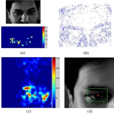
meaning that the objective function only considers pixels that have been previously selected as eye centre candidates. The displacement vectors and gradient vectors are normalised to unit vectors. This objective function is modified such that a gradient vector is only considered if its direction is reverse to the displacement vector. This is based on the observation that the pupil is always darker than its neighbouring regions and thus generates outward gradients. A sample implementation of this approach on an eye image is illustrated in Fig. 11. We tested this modality on a number of images with varied head poses, gaze directions and partial eye/pupil occlusions. The raw face images (right halves), gradients from the eye regions, and the corresponding energy maps are shown in Fig. 12.

Fig. 11. A sample implementation of the second modality using local gradient features. (a) An eye image where the localised eye centre is displayed. (b) The gradient magnitude image where gradient directions are represented by arrows. Gradients with magnitude below 70% of the maximum are removed (c) The resulting energy map for eye centre candidates.

While this method provides an effective solution to eye centre estimation, it has a number of inherent limitations that would incur error or even failure in the estimation. First of all, the objective function is formulated given that the pupil and the iris are circular objects. When the edges around eye corners and shadows surpass the pupil and the iris in circularity measure, they will cause eye centre estimates to be located on themselves rather than the centre of the pupil. Secondly, gradients on eyelids, eye corners and eyebrows will also vote for eye centre estimations. We define these as ‘non-effective gradients’, as opposed to ‘effective gradients’ that are located on edges of the iris and pupil. In more severe cases where makeup and shadows are prominent, the iris and the pupil, by contrast, generate weak ‘effective gradients’ such that the energy map is prone to erroneous energy response. This will further escalate estimation errors.

To resolve the above problems shared by most methods that utilise geometrical features for eye centre localisation, we introduce a radius constraint and design a SOG filter that can effectively deal with circularity measure and can resolve problems posed by eye corners, eyebrows, eyelids and shadows.

4.3 Iris radius constraint

A radius constraint is introduced such that the Euclidean norms of displacement vectors, which are related to estimated iris radius, have more influence on the calculation of an eye centre location. This is based on the assumption that shadows and eyebrow segments have random radius values, while the iris radii are more constant relative to the size of a face. This provides a way to differentiate circular clusters of various radiuses and to determine their weights in energy map accumulation. The function for the significance measure emulates the frequency response of a Butterworth low pass filter:

𝑤𝑟(𝑥, 𝑦) = _√ 1

1 + (‖𝒅(𝑥, 𝑦)‖2− ρ

𝜔 )

2𝜎

2 ₍₁₉₎

where ‖𝒅(𝑥, 𝑦)‖2 is the 𝐿2 norm of a displacement vector without being normalised to unit vector. ρ is the estimated radius

of the iris. 𝜎 and 𝜔 correspond to the order and the cutoff frequency of the filter. The curves corresponding to varying 𝜎 and 𝜔 following equation (19) are shown in Fig. 13. It should be noted that in each subfigure only one parameter is variable while the other remains constant.

Fig. 13. The radius weight function curves emulating the frequency responses of a Butterworth low pass filter. (a) Curves with varying 𝜎

(𝜎 = 1, 2 , 3) and constant 𝜔 (𝜔 = 2). (b) Curves with varying 𝜔 (𝜔 = 1, 2 , 3) and constant 𝜎 (𝜎 = 2).

4.4 Selective Oriented Gradient filter

With the inspiration drawn from the histogram of oriented gradients (HOG) feature descriptor [53], a SOG filter is introduced that discriminates gradients of rapid change in orientation from those of less change. We specifically design this novel SOG filter and introduce it into the modular eye centre localisation scheme so that it is perfectly tailored to reinforce the two main modalities despite its versatile applicability. The basic idea takes the form of a statistical analysis of the gradient orientations within a window centred at a pixel position. For each 𝐾𝑥× 𝐾𝑦 window (12×8 pixels in the experiment)

centred at pixel 𝑖, the gradients in 𝑥 and 𝑦 directions are calculated, whose orientations follow:

𝛳 = tan−1₍𝐼𝑦

𝐼𝑥)∙

180°

𝜋 (20)

The gradient orientations are then accumulated into 𝑘 (𝑘 < 360) orientation bins, where each bin contains the count of orientations from 𝑏 ∙360°_𝑘 to (𝑏 + 1) ∙360°

𝑘 (0 ≤ 𝑏 ≤ 𝑘 − 1) within the window. If the recorded count in a bin exceeds a

threshold, the corresponding pixels that accumulate the bin will have their gradient vectors halved, i.e. their weights reduced. As a result, the objective function becomes:

𝒄∗₌arg 𝑚𝑎𝑥

𝒄 {

1

𝑁∑ ∑ 𝑤𝑔(𝑥, 𝑦) ∙ 𝑤𝑟(𝑥, 𝑦) ∙ [𝛼 − 𝐼(𝑥, 𝑦)] ∙ (𝒅𝑻

𝑛

𝑦=1 (𝑥, 𝑦) ∙ 𝛻𝐼𝒄(𝑥, 𝑦))

2 𝑚

𝑥=1 } (21)

where 𝑤𝑔(𝑥, 𝑦) is the weight of a gradient adjusted by the SOG filter (i.e. 𝑤𝑔(𝑥, 𝑦) = 0.5 to halve the gradient vectors and

𝑤𝑔(𝑥, 𝑦) = 1 otherwise). The threshold for the counts is determined by an absolute value (6 in the experiment) as well as a

value (40% in the experiment) relative to the number of pixels with non-zero gradients within the window. As a result, pixels that maintain similar gradient orientations to their neighbours will have their weights reduced and they are referred to as ‘impaired pixels’ in the rest of the paper. When a curve has low curvature, it comprises more ‘impaired pixels’. Therefore the SOG filter can be used for general curvature discrimination tasks. It has the advantage that it does not require an explicit function for the curve and that it is effective in dealing with curves forming irregular shapes. Fig. 14 demonstrates the effectiveness of a SOG filter applied to an image containing irregular curves and an image of an eye region.

Fig. 14. Gradient filtering using a SOG filter. (a) An example of curved shape detection using a SOG filter where the ‘impaired pixels’ are detected. (b) An example where a SOG filter is applied to an eye image. The edges on the eye pouch and eyelids are successfully detected.

orientation of gradients to serve for gradient filtering. It resolves the challenges brought by shadows, facial makeup and edges on the eyelids, eyebrows and other facial parts outside the iris that are most interfering in geometrical feature based eye centre localisation approaches.

4.5 Energy map integration

In the final stage, two energy maps 𝐸𝑎 and 𝐸𝑏 are integrated into 𝐸𝑓(𝑥, 𝑦) so that they both contribute to election of an

eye centre. It is critical, prior to the integration, to determine the confidence of each modality, to estimate the complexity of the eye image, and thus to determine their weights in the fusion mechanism.

The left eye region is taken as an example to illustrate the fusion mechanism. If the equivalent centroid 𝐶𝑎𝑢𝑙calculated

by equation (16) is close to the pixel position 𝐶𝑚𝑎𝑥𝑙 that has the maximum value in the first energy map 𝐸𝑎𝑢𝑙(𝑥, 𝑦), 𝐶𝑎𝑢𝑙 is

considered confident since the isophote centre and the equivalent centroid coincide. In this case, more ‘effective gradients’ are present, allowing the second modality to be more robust and precise. The two modalities are then utilised and fused following equation (22). When 𝐶𝑎𝑢𝑙 and 𝐶𝑚𝑎𝑥𝑙 disagree and have a large Euclidean distance, the first energy map will have

high energy clusters sparsely distributed, potentially caused by severe shadows and specularities. The second modality will be influenced by ‘impaired pixels’ and produce erroneous centre estimates. Therefore only the equivalent centroids 𝐶𝑎𝑢𝑙 and

𝐶𝑎𝑢𝑟 are selected as final eye centres.

𝐸𝑓(𝑥, 𝑦) = _‖𝐶 1

𝑎𝑢𝑙 − 𝐶𝐸𝑎𝑚𝑎𝑥‖2∙ 𝐸𝑎(𝑥, 𝑦) + 𝐸𝑏(𝑥, 𝑦) (22)

where 𝜖 takes a value relative to the width of the eye region 𝜖𝑓 and 0 < ‖𝐶𝑎𝑢𝑙− 𝐶𝐸𝑎𝑚𝑎𝑥‖2≤ 𝜖. In our experiments,

𝜖 = 0.3𝜖𝑓 pixels. The maximum response in the final energy map will represent the estimated eye centre. The estimate for

the final right eye centre follows the same approach.

4.6 Eye centre localisation experiments and results

The public dataset used is the BioID database [52], consisting of 1520 images. It has been popular in the literature for evaluations of other eye centre localisation algorithms. The variations in the database include illumination, face scale, head pose and presence of glasses. Applied to this database, the proposed algorithm was tested against the others in the literature in resolving challenges introduced by the wide range of variations. The relative error measure proposed by [54] was used to evaluate the accuracy of the algorithm. This method firstly calculates the absolute error, i.e. the Euclidian distance between the centre estimates and the ground truth provided by the database; it then normalises the Euclidian distance relative to the pupillary distance. This is formulated by equation (23).

𝑒 = max(𝒹𝑙𝑒𝑓𝑡, 𝒹𝑟𝑖𝑔ℎ𝑡)

ɛ (23)

where 𝒹𝑙𝑒𝑓𝑡 and 𝒹𝑟𝑖𝑔ℎ𝑡 are the absolute errors for the eye pair, and ɛ is distance between the left and the right eye, i.e. the

pupillary distance, measured in pixels. The maximum of 𝒹𝑙𝑒𝑓𝑡 and 𝒹𝑟𝑖𝑔ℎ𝑡 after normalisation is defined as ‘max normalised

error’ 𝑒𝑚𝑎𝑥. Similarly, the accuracy curve for the minimum normalised error 𝑒𝑚𝑖𝑛 and the average normalised error 𝑒𝑎𝑣𝑔 are