I
Research on Intelligent Controller Design for MIMO
Spatially-Distributed Systems with Applications
YIZHI WANG
A thesis submitted in partial fulfilment of the requirements of the University of the West of England, Bristol for the degree of Doctor of Philosophy.
Faculty of Environment and Technology, University of the West of England, Bristol
Spatially dynamic distributed systems have been attracting increasing attention from researchers in the field of system modelling and control since their introduction as an alternative to simple systems to meet the ever-greater requirements to make industrial systems more precise and energy-efficient and to overcome process complexities. An approach whereby complex systems with multi-dimensional parameters, inputs or outputs are simply disregarded or simplified with the help of convenient mathematical models is no longer feasible. Therefore, the purpose of the present study is to contribute to the advancement of both theoretical and empirical knowledge in this field through the means of theoretical analysis, application simulations and case studies.
From a theoretical perspective, this study focuses primarily on the design methodology of control systems. To this end, the first step is identification of requirements from the applications, followed by the implementation of an original approach underpinned by data prediction for type-2 T-S fuzzy control with the purpose of making the control system design more convenient. With this aim in mind, the study creates an interface/platform to link or anticipate spatially dynamic distributed system output from lumped system data by taking advantage of the three-dimensional character of type-2 fuzzy sets. Moreover, on the basis of a decoupled spatially dynamic distributed system, this study applies Mamdani-type and interval type-2 T-S type fuzzy control, and extends a discussion about the results of simulation and analysis.
III
expand the SISO system into a MIMO system and the interacted inputs and outputs have been decoupled using decoupling method; and then a Mamdani-type fuzzy control was designed for temperature control and an Interval Type-2 fuzzy control was designed for pressure control, using a simple state-space model instead of a fuzzy model, accordance with the practical plant in use, and very satisfied, very robust control performances were obtained.
I would like to take this opportunity to express my sincere gratitude to my supervisors, Professors Quanmin Zhu and Mokhtar Nibouche, for their encouragement and guidance during the past years of my studies not only to my research but also to my English, and I also give my thanks to staff from the Faculty of Environment and Technology of UWE with whom I share the excellent and comfortable research environment.
I would like to extend my gratitude to my progression reviewer, Professor Yufeng Yao from the UWE, who gave me so much instructive advice and useful suggestions on my thesis; and my gratitude to Dr. Pritesh Narayan from UWE who gave me the most valuable comments on my thesis; to Professor Shaoyuan Li, who spares no effort in sharing ideas and guidance with my research; to PhD candidates Xin Liu, with whom I shared constructive discussions; to Postgraduate students Rui Li, Ji Qiu, Ge Zhu and Jieying Zhong, my classmates from UWE, who provided great help and support in both my study and my convenience life in UK; to Professor Fengxia Xu and Professor Hong Zhang who has given me constant support and care all the time.
Most importantly, I must say that nothing of this thesis would have been possible without the loving support of my parents and my husband, I will be indebted to them forever.
V
[image:5.595.111.528.214.739.2]ABSTRACT ... II ACKNOWLEDGEMENT ... IV TABLE OF CONTENT ... V NOMENCLATURE ... VIII LIST OF FIGURES ... IX
1 INTRODUCTION ... 1
1.1 OVERVIEW ... 2
1.2 MOTIVATION ... 4
1.3 RESEARCH QUESTIONS ... 6
1.3.1 Modelling: how can a SISO system be expanded into a MIMO system? ... 6
1.3.2 How can the coupled nature be solved? ... 7
1.3.3 How can the energy consumption be reduced? ... 7
1.3.4 How can type‐2 fuzzy control be implemented? ... 7
1.4 CONTRIBUTIONS ... 8
1.5 STRUCTURE OF THESIS ... 9
1.6 PUBLISHED PAPERS ... 10
2 BACKGROUND AND LITERATURE REVIEW ... 11
2.1 SPATIALLY DYNAMIC DISTRIBUTED SYSTEMS ... 12
2.1.1 Introduction ... 12
2.1.2 Development ... 14
2.1.3 Applications and Problems ... 16
2.2 STATE‐SPACE APPROACH ... 17
2.2.1 Definition ... 17
2.2.2 Applications ... 21
2.2.3 Recent Research Outcomes ... 22
2.2.4 Discretization ... 23
2.3 FUZZY LOGIC AND FUZZY CONTROL ... 24
2.3.1 Introduction ... 24
2.3.2 Fuzzy Logic ... 25
2.3.3 Mamdani Fuzzy Control ... 35
2.4.1 Application... 49
2.4.2 Description ... 50
2.5 CONCLUSION ... 52
3 METHODOLOGY ... 54
3.1 STATE SPACE MODELLING APPROACH ... 55
3.1.1 Model assumption ... 55
3.1.2 System Identification ... 56
3.2 POLE PLACEMENT CONTROL... 56
3.2.1 Assign closed loop poles ... 57
3.2.2 Assign closed loop zeros ... 58
3.3 DECOUPLING CONTROL ... 59
3.4 MAMDANI FUZZY CONTROL ... 62
3.5 INTERVAL TYPE‐2 FUZZY CONTROL ... 64
3.5.1 Interval Type‐2 Fuzzy Control ... 64
3.5.2 Type‐2 Fuzzification ... 65
3.5.3 Inference ... 65
3.6 CONCLUSIONS ... 67
4 PLANT MODELLING ... 69
4.1 PLANT MODELLING ... 70
4.1.1 Plant Analysis ... 71
4.1.2 State Variable Determination ... 75
4.1.3 State Space Equations ... 76
4.1.4 Control System Design ... 78
4.2 POLE PLACEMENT STATE FEEDBACK SYSTEM DESIGN ... 81
4.2.1 Observability ... 81
4.2.2 Controllability ... 82
4.2.3 Matrix Transformation ... 83
4.3 DECOUPLING CONTROL SYSTEM DESIGN ... 89
4.4 CONCLUSIONS ... 90
5 CONTROL SYSTEMS DESIGN ... 92
VII
5.1.3 Fuzzy Rule Base ... 96
5.1.4 Maximum of Membership Approach ... 98
5.2 TYPE‐2 FUZZY CONTROL SYSTEM DESIGN ... 98
5.2.1 Fuzzification ... 98
5.2.2 Inference ... 100
5.2.3 Rule Base ... 101
5.3 CONCLUSIONS ... 102
6 SIMULATION RESULTS AND ANALYSIS ... 103
6.1 SYSTEM PERFORMANCE... 104
6.1.1 SISO (temperature) System Performance ... 105
6.1.2 MIMO (Temperature and Pressure) System Performance (state feedback) ... 107
6.1.3 pole placement design ... 109
6.1.4 Time Response for decoupling design ... 112
6.2 CONTROL SYSTEM PERFORMANCE ... 116
6.2.1 Mamdani‐Temperature Control Performance ... 116
6.2.2 Type‐2 Interval Fuzzy Control System Performance ... 118
6.3 COMPARISON OF PERFORMANCE ... 121
6.3.1 Comparison for temperature control ... 121
6.3.2 Comparison for Pressure Control ... 122
6.4 CONCLUSIONS ... 123
7 CONCLUSIONS AND FUTURE WORK ... 125
7.1 CONCLUSIONS ... 126
7.2 FUTURE WORK ... 130
REFERENCE ... 132
Variables:
c Specific Heat Capacity J Kg C/ ( * )o
Q Quantity of heat J
M Mass of object Kg
T Temperature oC
t
Time sS Area m2
d Diameter m
Density Kg m/ 3h Height m
q
Subscript:
Volume rate Constant
m3
J/m3
o Object (here refers to vials) a
p
IX
FIGURE 2‐1 GENERAL DIAGRAM FOR STATE SPACE MODEL ... 19
FIGURE 2‐2 GENERAL DIAGRAM OF STATE FEEDBACK APPROACH ... 21
FIGURE 2‐3 BLOCK DIAGRAM OF GENERAL FUZZY CONTROL SYSTEM ... 36
FIGURE 2‐4 GENERAL DIAGRAM OF FUZZY CONTROL SYSTEM ... 37
FIGURE 2‐5 2‐D MAMDANI TYPE CONTROL BLOCK DIAGRAM ... 37
FIGURE 2‐6 T‐S TYPE CONTROL BLOCK DIAGRAM ... 42
FIGURE 2‐7 THE STRUCTURE OF TYPE‐2 FUZZY CONTROL ... 44
FIGURE 2‐8 COMPARISON OF TYPE‐1 AND TYPE‐2 MEMBERSHIP FUNCTIONS (MENDEL ET AL, 2006) ... 45
FIGURE 2‐9 SYSTEMATIC DIAGRAM OF DEPYROGENATION TUNNEL ... 51
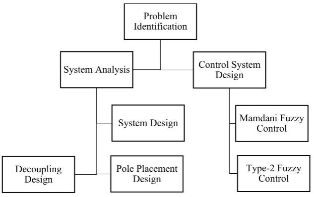
FIGURE 3‐1 DESIGN METHODOLOGY ... 54
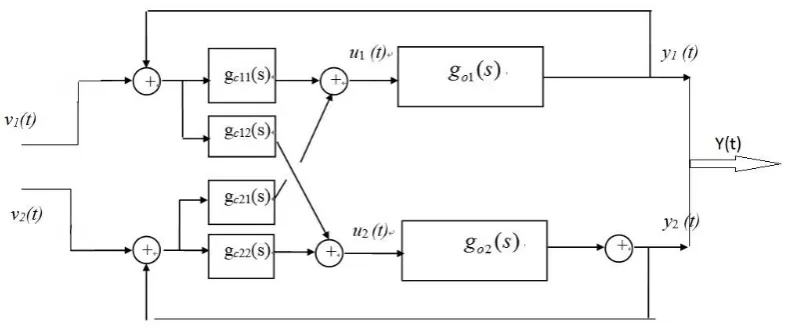
FIGURE 3‐2 GENERAL DIAGRAM OF DECOUPLING APPROACH ... 61
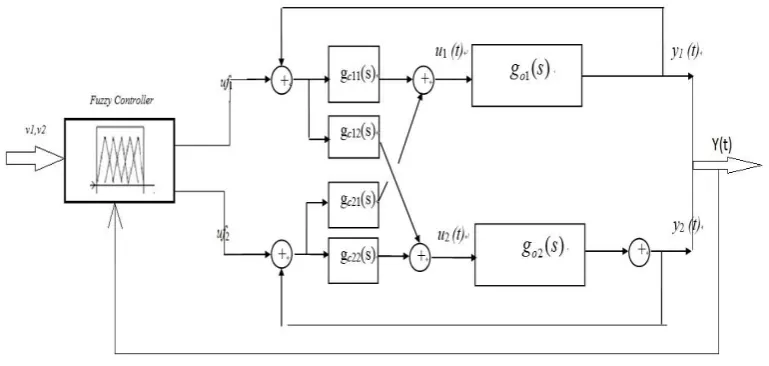
FIGURE 3‐3 GENERAL DIAGRAM OF FUZZY CONTROL ON DECOUPLING APPROACH ... 62
FIGURE 4‐1 SYSTEM ANALYSIS OF DEPYROGENATION TUNNEL ... 71
FIGURE 4‐2 PRESSURE ANALYSIS ... 74
FIGURE 4‐3 BLOCK DIAGRAM OF STATE SPACE ... 84
FIGURE 4‐4 BLOCK DIAGRAM OF STATE SPACE AFTER TRANSFORMATION ... 84
FIGURE 5‐1 MEMBERSHIP FUNCTION FOR INPUT VARIABLE E1 ... 94
FIGURE 5‐2 MEMBERSHIP FUNCTION FOR INPUT VARIABLE EC1 ... 95
FIGURE 5‐3 MEMBERSHIP FUNCTION FOR OUTPUT UF ... 96
FIGURE 5‐4 MEMBERSHIP FUNCTION FOR PD ... 99
FIGURE 5‐5 SECONDARY VARIABLES (COORDINATES)... 100
FIGURE 6‐1 TIME RESPONSE FOR SISO STATE SPACE MODEL UNDER 0.5,0.8, 1 ... 107
FIGURE 6‐2 TIME RESPONSE FOR SISO STATE SPACE MODEL UNDER U=1 AND NOISES ... 107
FIGURE 6‐3 SYSTEM RESPONSE FOR MIMO STATE‐SPACE MODEL (V1=1.5,V2=0.5) ... 108
FIGURE 6‐4 SYSTEM RESPONSE FOR MIMO STATE‐SPACE MODEL (V1=3, V2=0.5) ... 109
FIGURE 6‐5 TIME RESPONSE FOR POLE PLACEMENT ... 111
FIGURE 6‐6 TIME RESPONSE FOR DIFFERENT V1 VALUES ... 112
FIGURE 6‐7 TIME RESPONSE FOR DIFFERENT V2 VALUES ... 113
FIGURE 6‐8 TIME RESPONSE FOR DECOUPLING CONTROL ... 114
FIGURE 6‐9 DECOUPLING CONTROL WITH NOISES ... 115
FIGURE 6‐10 MAMDANI TYPE FUZZY CONTROL FOR TEMPERATURE ... 116
FIGURE 6‐11 MAMDANI TYPE FUZZY CONTROL WITH NOISES ... 117
1
Introduction
1.1
Overview
Advances and developments in medicine and medical treatment have led to a longer human lifespan and a lower death rate. For instance, drugs of higher purity have a better healing effect, such as more accurate efficacy, or relieve symptoms more effectively, or even contain fewer side-effects. However, the effectiveness of each section of manufacture can influence the desired results either positively or negatively, and sometimes such an influence is linked to multiple disciplines rather than a single cause and effect. Partially, such increasing multi-disciplinary requirements have directly promoted the development of pharmaceutical engineering, as one of the important factors. In addition, different from the chemical pharmaceutical process, the biochemical pharmaceutical process presents a more complicated nature, due to its complex biochemical reactions, such as more than one reactor involved in a single reaction, as well as the time-delay, unobservable and hardly controllable process during manufacture. Along with such nature, the biochemical pharmaceutical industry has transformed itself throughout the years, with its technologies and processes expanding and changing constantly to suit today’s needs. The development process for high performance equipment for use in the industry has now become subject to tighter and stricter regulations, especially for safety concerns, and this in turn has made the control process of such equipment more demanding, complex and challenging. The control process must ensure the highest form of purity of the products going through the machine, all while reducing the overall consumption of energy and raw materials (Koveos et al., 2013).
widely accepted in the biochemical pharmaceutical industry and exclusively intended for sterilisation and drying of vials and syringes conveyed through it is the depyrogenation tunnel. This device can consume a large amount of power resources when in operation, and thus, energy consumption has become an important factor when designing a depyrogenation tunnel along with its control system design. To minimize power consumption and to maintain its reliability of the sterilisation process, modelling and control strategies are required. The unstable pressure field within the depyrogenation tunnel is an additional key issue, alongside the temperature issue. As the vials are conveyed through, the open zone within is connected with the room, which will be affected significantly by the combination of room pressure and wind pressure. In other words, if the pressure fluctuates beyond a certain value, the small vials made of glass are likely to fall off, causing the device to stop and resulting in significant loss. In addition, more critical than the issue of energy consumption is the issue of physical structure deficiency caused by the complex nature of the device and known as a spatially dynamic distributed system.
The spatially dynamic distributed system has attracted considerable research attention in recent years. Using the depyrogenation tunnel as an instance, for safety concerns, the equipment shall be validated to ensure that every item conveyed through it will satisfy the requirements of temperature and time. However, in order to reduce costs, the structure of this equipment is designed as a lumped parameter system. Meanwhile, the design is also deficient in the validation method. So far, there is no such efficient and theoretically feasible test method to validate the results. Instead, operators are using a practical method (e.g. periodically conducting comparison test). Thus, in order to pass the comparison test (and also meet the manufacture requirements), operators have to practically degrade the priority of energy consumption. For instance, they have to use a much higher temperature at the check point to ensure the test results.
many scientists successfully established a variety of methods for constructing efficient, robust, flexible and general purpose control system approaches, such as PID control, optimal control, robust control, self-adapted control, fuzzy control, neural network-based control, expert control, and various combinations of them. In recent years, among these methods, the application of fuzzy system has become one of the most popular research interests in this area. Fuzzy control theory is a derivative from Professor Zadeh’s important research result in 1965, where he proposed the concept of fuzzy set known from traditional sets. More specifically, Zadeh (1965) assigned a degree to the traditional set that could decide the degree of the element belonging to the conventional set. This made it possible for computers to deal with human uncertainty and ambiguity. In this case, one of the significant applications evolved into fuzzy control theory. After years of development, the fuzzy control approach has been made suitable for the complex plants for non-model-based control system design method and many researchers have pushed this domain forward to many successes in both theory and practice. Henceforth, following the introduction of type-2 fuzzy sets by Zadeh in 1975, related applications and advancements were prompted to address a range of issues of high complexity, such as a spatially dynamic distributed system that cannot be simplified as a lumped parameter system.
1.2
Motivation
to deal with such issues: some complicated objects are easy to model in software and in laboratory application where researchers can assume infinite number of sensors to obtain many data. Some employ mathematical methods for simplification, whilst others sacrifice energy consumption in order to achieve the desired results. However, as mentioned above, along with the gradually complex requirements of the manufacture processes, it is not so feasible to install many sensors in such an object for the reason of manufacture cost; or so accurate after simplification when the object contains significant variables that cannot be idealized as known formulas; or so earthy to sacrifice energy consumption especially when it becomes the main kernel in view of the plant running cost. In conclusion, sometimes it is not feasible to obtain the effect from the cause via the cause-and-effect relationship. However, a different way of dealing with the effect can be conjured up. On some occasions, difficulties in obtaining precise models drive the other ways to meet the system design requirements. Under such prerequisites, it is significant to open up a snap course for such purposes. For the above-mentioned systems, and especially when it is not possible to accurately model them mathematically, control system design can focus on the results using servo method, such as fuzzy control.
Apart from the physical analysis and application design to deal with the identified issue, the theoretical challenges as associated with the spatial distributed system with MIMO nature and its control approaches are also identified. One of the challenges of this thesis is to make sure that there is a balance of accuracy and response within the system, so the total number of sensors used in the system needs to be limited to reduce the cost, but must still be high enough to retrieve the amount of data with acceptable levels of accuracy. In accordance with the complicated and even coupling nature of the variables associated with spatially dynamic distributed systems, the control system is designed to deal with the issues instead of considering the objects directly.
research is that there is a need to address the current concerns about designing principles and limitations. This project also aims to create a good balance between accuracy and the response the machine produces and to reduce the amount of energy the machine consumes to operate, which will ultimately reduce the total cost of machine operation. Having more sensors will allow more data with higher rate of accuracy. However, the downside of this is the lack of quick response from the machine. On the other hand, reducing the number of sensors used in a system will result in excellent system response, but it can adversely affect accuracy. This is usually known as a lumped parameter system.
1.3
Research Questions
The logical framework of the research, throughout the modelling and assumption and to the facilitation of control systems, is outlined in the following research questions.
1.3.1
Modelling: how can a SISO system be expanded into a MIMO system?1.3.2
How can the coupled nature be solved?After the expansion work is done, two inputs, two outputs and the two states, which is not a commonly seen, and standard mathematical state space model, are coupled together. That is to say, how can the coupled nature of this plant can be solved in case to facilitate the design of control systems?
1.3.3
How can the energy consumption be reduced?As for the practical-in-use plant, it is mounted with only two sensors, one for temperature control and one for pressure monitor. In other word, this plant is designed as a lumped parameter system, for cost-down purpose, as the more sensors, the more cost. in order to meet FDA’s requirements (to heat the vials to 300ºC and keep them for 5 minutes under this temperature), the most secure way is to set the desired temperature to 340ºC. And it is well known that to generate the high temperature environment even in a small space will consume large amount of energy, and even reference temperature is lower down by 1ºC, energy consumption will be accumulatively reduced. Therefore, the research question that how can the energy consumption be reduced is also a very practical issue to settle down.
1.3.4
How can type-2 fuzzy control be implemented?how to simplify the type-2 fuzzy control design process, such as the type-reduction process.
1.4
Contributions
The main contributions of this thesis are summarised as follows:
Based on a comprehensive literature review of both theory and practice, the concepts and the definitions of the related subjects are revisited and clarified with reasonable justifications/revisions and improvements demonstrated through descriptions and examples.
Expansion of the SISO spatially dynamic distributed system to MIMO spatially dynamic distributed system, to introduce another variable based on the existing physical structure of the machine.
The creation of a platform for a MIMO spatially dynamic distributed system control scheme.
Development of a solution to the system’s coupling nature
Application of matrix transformation to expand the SISO pole placement method to MIMO pole placement
Controlling the decoupling system based on the design of a Mamdani-type fuzzy control scheme
1.5
Structure of Thesis
This thesis is divided into seven chapters. Apart from Chapter 1, which is the overview and introduction to this research, and Chapter 7, which provides the conclusions drawn from the research and recommendations for further study, the rest of the chapters are separated into two parts, namely, theoretical study and application area design and development. Chapters 2 and 3 provide the background and methodology for the research thesis, respectively; Chapter 4 is concerned with the application area design and development, including model expansion design, pole placement control and decoupling control design; Chapter 5 addresses the theory-based study of fuzzy control and type-2 fuzzy control system design, which will be facilitated for MIMO spatially dynamic distributed system, and the designed fuzzy control system will be validated with the model established in Chapter 4; Chapter 6 presents the simulation results and analysis, finalising the research content. The outline of the thesis is as follows:
Chapter 1 Introduction and outline of the thesis.
Chapter 2 The literature review covers the practical and theoretical background, including research related to the modelling and simulation of MIMO spatially dynamic distributed systems based on the conventional control theory, as well as conventional and type-2 fuzzy control to tackle the problems of control of spatially dynamic distributed systems.
Chapter 3 The fundamental knowledge and preliminary methodologies related to the research work in this thesis are set out, and some concepts and definitions are clarified.
Chapter 5 The mathematical analysis and control system design for MIMO spatially dynamic distributed systems is achieved using the data-based predictive control approach. Furthermore, this chapter is also concerned with the development of an interval type-2 fuzzy control framework without reliance on objects.
Chapter 6 Comparison and analysis of the simulation results.
Chapter 7 Conclusions and recommendations for further research.
1.6
Published Papers
1) Y. Z. Wang, Q. M. Zhu and M. Nibouche, “State-Space Modelling and Control of a MIMO Depyrogenation Tunnel”, accepted by 34th Chinese Control Conference and SICE Annual Conference 2015 (CCC&SICE2015),27-31, July, Hangzhou.
2) Y. Z. Wang, Q. M. Zhu and M. Nibouche, “Mamdani Type Controller Design for MIMO Systems with Case Study”, accepted by 7th International Conference of Modelling, Identification and Control 2015 (ICMIC 2015), 18-20, December, Tunisia.
2
Background and Literature Review
2.1
Spatially Dynamic Distributed Systems
2.1.1 Introduction
The system identification is an art and the science for constructing a mathematical model of a system (Ljung, 2010). From one perspective, a suitable mathematical model will afford comprehensive insight into system structure and core elements, thus ensuring ample data on consequential sections, signal transmission, controller design and other aspects. The system identification and modelling should be the foundation of all work, because a well-designed system model will deliver the most elaborate precision in validation output for a proposed controller.
As the software industry is becoming increasingly more developed, various reputable applications have begun to be exploited for the purposes of system modelling. Generally, AutoCAD is proper to graphic design and ANSYS is tailored for finite element design, which is extensively used in industrial design. Matlab, as one of the powerful simulation tools in system design, provides capacious space and freedom for engineers to construct their own options. In conclusion, the problem is how to identify the system and what software to use to model it.
and he conducted further study on the definite theory of the partial differential equations, which was used to describe the distributed parameter systems, including elliptic type, parabola type and hyperbolic type of partial differential equations.
As the control of spatially dynamic distributed systems is becoming an increasingly prominent research field, an abundance of research results is being produced. The relevant analysis of optimal control, tuning, random control, self-adaptive control, robust control is gradually supplemented in the control of linear spatially dynamic distributed systems and the important theories of stability, controllability and observability have been perfected in this field as well (Curtain, 1978). The main research methods of linear spatially dynamic distributed systems consist of abstract space theory, functional analysis, spectral method, frequency domain analysis methods, finite difference method and finite element method, among others.
Consequently, in keeping with the developmental trajectory of contemporary science and technology as well as practical engineering control systems, the control of non-linear spatially dynamic distributed systems has been the focus of ample research and analyses, fostering the development and implementation of effective control methods. These methods include the stability control based on Lyapunov (Christofides, 2001), PID control (Alvarez, 2001), model control (Chen and Chang, 1992), geometric control (Kravaris, 1991), control based on finite dimension system theory (Hoo, 2001), model predictive control (Zheng, 2004), self-adaptive control (King, 2003), sliding model control (Sira, 1989) and optimal control (Park, 1995). Meanwhile, some methods that were originally intended for linear spatially dynamic distributed systems are now used in the controller design of non-linear spatially dynamic distributed systems.
pressure field identified from these two examples are two typical cases of spatially dynamic distributed systems. In general, spatially dynamic distributed system is considered as a system with parameters that span over space and time, which means that, within a certain space and within a certain period of time, the parameters vary with time, or space, or both. As a result, spatially dynamic distributed system is also known as parameter distributed system. Hence, when considering the Energy Conservation Law, most of the spatially dynamic distributed systems can be represented as follows:
2 2
2 2
(z, t, x, , , , ,..., , ) 0
n n
n n
x x x x x x
F
z t z t z t
(2.1.1)
Where z and t are independent variables, z [ , ] l la b denotes the variable of space, and ,
a b
l l are constants, t0 denotes the time constant, x is the dependent variable, therefore ( )F is a nonlinear function with regard to the independent variables z and t, dependant variable x, and partial derivative formula of x with regard to independent variables from the first order to n-order.
2.1.2 Development
with lumped parameter systems. Meanwhile, he utilized the moment method to optimally control spatially dynamic distributed systems. Subsequently, Lions (1971) developed the optimal control and identification theory of spatially dynamic distributed systems, and he conducted further study on the definite theory of the partial differential equations, which was used to describe the distributed parameter systems, including elliptic type, parabola type and hyperbolic type of partial differential equations.
As the control of spatially dynamic distributed systems is becoming an increasingly prominent research field, an abundance of research results is being produced. The relevant analysis of optimal control, tuning, random control, self-adaptive control, robust control was gradually supplemented in the control of linear spatially dynamic distributed systems and the important theories of stability, controllability and observability have been perfected in this field as well (Curtain, 1978). The main research methods of linear spatially dynamic distributed systems consist of abstract space theory, functional analysis, spectral method, frequency domain analysis methods, finite difference method and finite element method. Glowinski et al. (2008) provided an overview of quantitative research conducted on the controllability of distributed parameter systems as well as applications.
The research and development on partial differential equations and functional analysis support the theoretical research of distributed parameter systems as well as providing the research with powerful analysis tools. Until now, research on the tuning, optimal control, controllability, observability, identity of distributed parameters and filtering of partial distributed systems has achieved similar results to lumped parameter systems, which can be considered as an expansion of relevant research results.
analyses, fostering the development and implementation of effective control methods. These methods include the stability control based on Lyapunov (Christofides, 2001), PID control (Alvarez, 2001), model control (Chen and Chang, 1992), geometric control (Kravaris, 1991), control based on finite dimension system theory (Hoo, 2001), model predictive control (Zheng, 2004), self-adaptive control (King, 2003), sliding model control (Sira, 1989) and optimal control (Park, 1995). Meanwhile, some methods initially intended for linear spatially dynamic distributed systems are now used in the controller design of nonlinear spatially dynamic distributed systems.
2.1.3 Applications and Problems
In engineering, it occasionally happens that control objects may need to be altered as distributed parameter systems due to the control system structure or actuators. For instance, if a hydraulic pressure actuator or pneumatic actuator is designed with complex structure or requires over distance, when performing modelling according to the actuator movement principle, the state transition of fluid or other media must be considered as well. Furthermore, such state transition is also described by a distributed parameter, which is not expected. In practice, the parameter-distributed controller is seldom adopted due to the difficulty involved in implementing it. In most cases, the control objects are parameter-distributed systems when a lumped parameter system serves as controller. There are generally three types of control approaches for distributed parameter systems:
1) Point control approach: put the control effort on several independent points of control objects, such as light control panel in a room;
sub-3) Boundary control approach: put the control effort on the boundary of the control objects, such as flooring heating system.
However, existing studies present obvious shortcomings. On the one hand, in the area of distributed parameter systems, research results are still far away from application in practice. On the other hand, a large gap in the research on spatially dynamic distributed systems remains to be filled, namely, systems with spatially dynamic distributed inputs and outputs.
2.2
State-space Approach
The state-space modelling approach is probably one of the most powerful modelling methods associated with the modelling and control of MIMO systems. This approach has undergone numerous developments over the years and has been successfully applied to many MIMO systems (Gueguen et al., 1985; Cassell and Choi, 2012). Due to its convenient transformation and simplification, the state-space approach is the preferred approach for characterising systems with dynamic parameters.
2.2.1 Definition
more nth-order differential or difference equations. Systems theory is the main foundation of the state-space model. Its early applications include famous programs like the Apollo and Polaris aeronautics and aerospace programs (Hutchinson, 1984). For example, it has seen application in the Kalman filter, which is an algorithm developed based on the work conducted by Kalman (1960, 1963). One version of the Kalman filter, known as the Kalman-Bucy filter (named after Richard Snowden Bucy), which is a continuous time version of the Kalman filter, has its algorithm based on the state-space model. It uses the measured data to decrease or even eliminate stochastic disturbance, and rebuilt the dynamic matrix (Gu and Yung, 2013). The state-space model used in Kalman filter takes measured data as recursive state variables. The state-space model has also been used in fuzzy logic control, especially in the Takagi-Sugeno (TS) inference type (Wang et al., 2015). Apart from the previously-mentioned scientific and engineering applications, the state-space model has also been used in other industries, such as finance (Mergner, 2009).
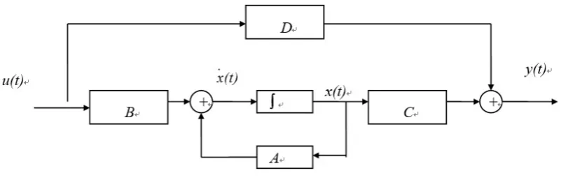
Figure 2-1 General Diagram for State Space Model
In a state-space model, the state of a system represents the very core of the model. A state of a system can be described as the current value of an internal element of a system, which changes its values independently from the system output. When using the state-space equations to model a system, three vectors need to be defined beforehand:
Input Variables: These represent the inputs of the system. The type of system that is being modelled will determine the number of inputs that need to be defined. In general, there are two possible systems: SISO (single input single output) and MIMO (multiple input multiple output). In SISO systems, only one input variable needs to be defined, while in a MIMO system, more than one of inputs can to be defined. Once all the inputs have been defined, they need to be arranged in a vector form.
Output Variables: These represent the outputs that the system produces. In a SISO system, only one output is produced, whereas in a MIMO system, more than one output is produced. The output variables are dependent on a combination of the input vector and the state vector. The outputs should be ideally independent of any of the others. That is, one input variable should only affect one output variable.
The state-space model has been developed over a long period of time and it is one of the most powerful modelling methods in dealing with complex MIMO systems (Wang et al., 2015). MIMO systems that are linear and lumped can be easily represented using the state-space approach.
Let S be the state-space model, then the general representation of S is as follows:
( , , , ) : ( ) ( ) ( ) ( )
( ) ( ) ( ) ( )
S A B C D x t Ax t Bu t State Equation y t Cx t Du t Output Equation
(2.2.1)
The inputs, outputs, and state variables are defined respectively as follows:
1 1 1
( ) [ ( ) ... ( )] ( ) [ ( ) ... ( )] ( ) [ ( ) ... ( )]
T m
T l
T n
u t u t u t y t y t y t x t x t x t
(2.2.2)
The matrices A, B, C and D are defined as follows:
Dynamic Matrix An n* : Also known as the state matrix, it is generally used to describe the dynamics of the system as well as to control the trajectory of the state vector ( )x t .
Input Matrix Bn m* : denotes how each control input affects the state variables of the systems.
State Feedback Approach
Based on the open loop diagram, the closed loop with state feedback approach, which is different from the output feedback, is also generated, as shown in Figure 2-2 General diagram of State Feedback Approach
Figure 2-2 General diagram of State Feedback Approach
1
( ) ( ) ... m( ) T
v t v t v t (2.2.3)
Which is called reference vector and it should be noticed that there are two gain matrices are introduced,
Fs is the m*n state feedback gain matrix to specify the poles of the closed loop
system.
H: is the m*m input feedforward gain matrix to specify the zeros of the closed loop system.
2.2.2 Applications
system”. According to Zheng et. al (2009), there are times where such interaction is not desired in an organization and this has led to decoupled systems, where multivariable systems being in the limelight in the last decade or so. To design a decoupled system, one has to ensure that each input maps to one output, effectively creating single input/output (IO) channel.
In state observation, a system’s state space model is not a true feedback system and this means that a feedback mechanism that x’ relates to x represents a single internal mechanism to the plant. To put it simply, the matrices A, B, C and D are part of a single device and not separate “components” per se. These matrices are immutable, meaning that they cannot be altered during the operation of the machine since they are intrinsic parts of the plant (Siekmann et. al, 2015). However, if the entire plant has been modified, the matrices will change. Since the matrices are immutable, a method that modifies the system externally is needed, and that is the feedback loop. In a state feedback, the state vector’s value is returned back to the input channel of the system. If an external feedback element exists in the system, the system is a closed-loop system. If otherwise, the system is known as an open-loop system. (WikiBooks, 2015).
2.2.3 Recent Research Outcomes
Consequently, MIMO-based models need to be developed to complement the machine’s complex non-linear nature.
In this regard, one of the best models is the one proposed by Jiang (2008), which is a new multi-rate fuzzy control technique for a continuous-time non-linear system. Jiang (2008) used the lifted Takagi-Sugeno (T-S) fuzzy logic model for the plant’s construction, which involved linear matrix inequalities (LMIs) and a multi-rate input controller for the multiple T-S linear model. It was based on the design of local feedback controllers using optimal disk-pole (D-Pole) placement and showed promising results in the closed-loop control system. Another powerful model for modelling a MIMO system is the state-space model. Over the years, the state-space model approach has been successfully applied in many different MIMO systems (Gueguen et al., 1980; Cassell et al., 2012). In this case, it becomes a very sound solution when trying to implement that state-space model in the control system design of a depyrogenation tunnel.
2.2.4 Discretization
while time discretization involves dividing the time by ∆τ.
2.3
Fuzzy Logic and Fuzzy Control
2.3.1 Introduction
The accuracy of the acquired knowledge and the possibility to employ traditional control approaches of confirmed precision are both minimised as control objects are becoming increasingly more complex, non-linear, and presenting a hysteretic quality and coupling nature. As stated in the Exclusive Principle, the more complex a system is, the more difficult it is to obtain crispy results. In other words, complexity and clarity are mutually exclusive. However, the human brain has managed to overcome these problems successfully.
purpose of automatic control. Therefore, it introduces the theory of fuzzy control, which is a computer system control technology based on natural language control rules and fuzzy logic inference. Fuzzy control is theoretically independent from mathematical models of traditional control systems but relies greatly on experience manipulation and knowledge base. It is worth mentioning that, although fuzzy control and expert system are both based on knowledge from experts, the expert system transfers the human language symbols directly to computer language, while fuzzy control rules transfer the language into numbers or mathematical expressions in advance of utilization.
Due to its convenient application, fuzzy control theory has been widely accepted since the 1980s and 1990s. As mentioned before, the development of fuzzy control system minimizes the precise mathematical requirements.
2.3.2 Fuzzy Logic
1. Definition of fuzzy sets
: 0,1 , A( )
A U xa x
(2.3.1)
Where A denotes a fuzzy set or a sub-fuzzy set in the domainU ; A( )x denotes the degree of each element of x belonging to the fuzzy setA and is known as the membership function of element x in fuzzy setA. When x is a determined element
0
x , A( )x0 is denoted as the degree of membership against fuzzy setA. Such definition has given the degree to fuzzy set A, whose boundary is not clear from any determined element x0and made the degree mathematized. If memberships of any fuzzy set only have two values, 0 and 1, the fuzzy set A is sharpened as a traditional set. Obviously, a traditional set is a typical case for fuzzy sets.
2. Membership Functions
Before a fuzzy set can be defined, the membership needs to be defined first. However, there is no single definition of membership, but multiple ones, due to differences in perception and language.
After years of development and trial-and-test efforts, the most widely used membership functions are listed as follows:
1) Triangle
0
( , , , )
0
x a x a
a x b b a
f x a b c
c x
b x c c b
x c
2) Bell 2 1 ( , , , ) 1 b f x a b c
x c a (2.3.3)
Where c determines the central position of the function, and a, b determines the shape of function.
3) Gaussian 2 2 ( ) 2 ( , , ) x c f x c e
(2.3.4)
Where c determines the central position of the function and determines the width of the curve.
4) Ladder
0
( , , , , ) 1
0
x a x a
a x b b a
f x a b c d b x c
d x
c x d d c x d
(2.3.5)
Where requires a b and c d .
( ) 1 ( , , )
1 a x c
f x a c
e
(2.3.6)
Where a and c determines the shape of function, and the function is central symmetry with respect to the point ( ,0.5)a .
3. Fuzzy Relationship
1) Definition
Within the traditional set theory, if some relationship exists between the elements with regard to the two sets, then it is not difficult to describe that relationship with some functions. However, as stated by the definition of traditional sets, the relationship between two sets either exists or not. However, after expansion to fuzzy set theory, the relationship between elements in two fuzzy sets came to denote the degree to which the elements were correlated to each other, namely, the fuzzy relationship. The fuzzy relationship is defined as follows:
( , ) : [0,1]
R x y A B (2.3.
7)
Where R is a fuzzy subset in A B , and the relationship determines the degree of correlation between elements x in fuzzy set A and elements y in fuzzy set B. Therefore, ( , )R x y denotes the binary fuzzy relationship, and abbreviated as Fuzzy Relationship.
to Q denotes the fuzzy relationship from fuzzy set X to Z, which can be represented asP Qo .
4. Defuzzification
Defuzzification is a process whereby a single number is used to represent a fuzzy set. The single number shall be an element in the fuzzy set, and can, in a manner, represent the fuzzy set. The most commonly employed methods of defuzzification are outlined below:
1) Method of Area Centre (Centroid)
This method is designed to determine the centroid of the area encircled by the membership function curve and the horizontal coordinate, using the abscissa value of this point as the representation of the fuzzy set.
Suppose the membership function of fuzzy set A in domain U is ( ),A u u U . If the abscissa value of the centroid is ucen , then the value is calculated as follows:
( ) ( ) U cen
U
A u udu u
A u du
(2.3.8)If domain U is discrete as U
u u1, , ,2 L un
and the membership of uj is A u( )j , so that ucen can obtain as follows:1
1
( ) ( ) n
j j
j
cen n
j j
u A u u
A u
Despite being considerably accurate and reasonable, the centroid method is time-consuming in terms of calculation.
2) Bisector Method
This method first determines the area encircled by the membership function curve and the horizontal coordinate and then determines the abscissa value of bisector that can divide the area into equal parts. The abscissa value is used to represent the fuzzy set.
Suppose the membership function of fuzzy set A in domain U is ( ),A u u U . If the abscissa value of the bisector line is ubis and u[ , ]a b then the value is calculated as follows:
1
( ) ( ) ( )
2
bis
bis
u b b
a A u du u A u du a A u du
(2.3.10)If domain U is discrete as U
u u1, , ,2 L un
, the area under the membership function is triangles, ladders or squares; therefore, the matter is reduced to determining the position in relation to half of the area of elements. This method is widely used in fuzzy control design.3) Method of Maximum
If there are more than one point with the maximum value of membership, the abscissa value of the average value umom should be taken as the representation.
Suppose A u( ) max( ( ))j A u , where j1, 2,L ,n , and there are n points in the largest membership degree, therefore:
1 max
n
j j
u u
n
(2.3.11)
b. Largest Value of Maximum (LOM)
If there are more than one point with the maximum value of membership in the domain, the point with the largest absolute value among those points should be selected and its abscissa value ulom should be used for the representation.
Suppose A u( ) max( ( ))j A u , where j1, 2,L ,n , and there are n points in the largest membership degree; the point with the largest absolute value max(uj ) uk should be chosen, namely:
u
lom
u
k (2.3.12)c. Smallest Value of Maximum (SOM)
Similar to LOM, if there are more than one point with the maximum value of membership in the domain, the point with the smallest absolute value among those points should be selected, and its abscissa value of usom should be used for the
representation.
largest membership degree; therefore, the point with the largest absolute value min(uj) uk should be selected, namely: usom uk.
5. Fuzzy Inference and Implication Relationship
A fuzzy proposition is classified as a simple proposition if it cannot be divided into simpler propositions. Therefore, suppose A a( ) and B b( ) are two simple propositions; if there is a fuzzy dependant relationship between the two propositions, such as “if ( )A a , then ( )B b ”, the compound proposition is called fuzzy condition statement, also known as fuzzy condition proposition. Suppose ( )A a , ( )B b and
( )
U u are fuzzy propositions, therefore there are two types of widely used statements, namely:
1) If A, then U.
It indicates the proposition: if a is A, then u is U, or if A(a) then U(u), can be represented as AU .
In order to obtain the fuzzy implication relationship of AU, there are several widely used algorithms summarised as follows:
Zadeh algorithm:
( , ) ( )( , )
max((1 ( )), min( ( ), ( ))) (1 ( )) ( ( ) ( )) R a u A U a u
A a A a U u A a A a U u
(2.3.13)
( , ) ( )( , )
min( ( ), ( )) ( ) ( )
R a u A U a u
A a U u A a U u
(2.3.14)
Larsen Algorithm:
( , ) (
)( , )
( )* ( )
R a u
A
U a u
A a U u
(2.3.15)Bounded Sum Algorithm:
( , ) ( )( , )
1 ( ( ) ( )) min(1, ( ( ) ( )))
R a u A U a u
A a U u A a U u
(2.3.16)
Mizumoto-s Algorithm:
( , ) ( )( , )
1 ( ) ( )
0 ( ) ( )
R a u A U a u A a U u A a U u
(2.3.17)
Mizumoto-g Algorithm:
( , ) ( )( , )
1 ( ) ( )
( ) ( ) ( )
R a u A U a u
A a U u U u A a U u
(2.3.18)
as follows:
According to the Mamdani algorithm, the result of the fuzzy implication relationship ( , ) ( ) ( )
R a u A a U u , when ( )A a and ( )U u are discrete, will be a fuzzy subset of direct productA U , namely ( , )R a u (A U ) . In this case, the fuzzy relationship
( , )
R a u can be represented by a m n* fuzzy relationship matrix. Therefore, the process consists of two steps:
The first step involves performance of transposition of ( )A a to obtain A ar( ), which is a column vector. This is to ensure that every element ai in A matches with every ui in U .
The second step involves performance of calculation A a U ur( )o ( ) (choose the smaller one) as follows:
1
2
1 2
1 1 1 2 1
2 1 2 2 2
1 2 ( , ) ( ) ( ) ( ) ( ) ( ) ( ) ( ) ( ) ( ) ( ) ( ) ( ) ( ) ( ) ( ) ( ) ( ) ( ) ( ) ( ) ( ) ( ) ( ) ( ) ( ) ( ) ( ) ( ) ( ) ( ) T n m n n
m m m n
R a u A a U u A a U u A a U u A a
A a
U u U u U u
A a
A a U u A a U u A a U u
A a U u A a U u A a U u
A a U u A a U u A a U u
r o o o L M L L
M M M M
L
(2.3.19)
1 1 1 2 1
2 1 2 2 2
1 2 ( , ) ( ) ( ) ( ) ( ) ( , ) ( , ) ( , ) ( , ) ( , ) ( , ) = ( , ) ( , ) ( , ) n n
m m m n
R a u A a U u A a U u
R a u R a u R a u
R a u R a u R a u
R a u R a u R a u
r o L L
M M M M
L (2.3.20)
2) If A and B, then U.
It indicates the proposition if a is A and b is B, then u is U, or if A(a) and B(b) then U(u), which can be represented as A B U. The calculation is similar to the first type of proposition.
It is worth mentioning that either of the inference results U is a fuzzy set, which cannot be used directly until defuzzification.
The concept of fuzzy logic control (FLC) involves basing the design of a practical controller on qualitative system knowledge. FLC is generally applicable to plants whose mathematical model cannot be found, but the qualitative knowledge of experienced operators provides enough information for control system design. It is particularly suitable for those systems with uncertain and/or complex dynamics.
2.3.3 Mamdani Fuzzy Control
Figure 2-3 Block Diagram of General Fuzzy Control System
As shown in the figure, the fuzzy controller constitutes the core element of the control system. Furthermore, the input x1 r v and output u of the fuzzy controller are crisp numbers.
Figure 2-4 General Diagram of Fuzzy Control System
It is assumed that the fuzzy system has inputs xiXi (where i1, 2, ,L n) and outputs yjYj (where j1,2, ,L m). The inputs xi and the outputs yj are real numbers; they are also called “crisp”.
3) Mamdani Type Control
A typical Mamdani Type control system always contains the modules as shown in the following figure:
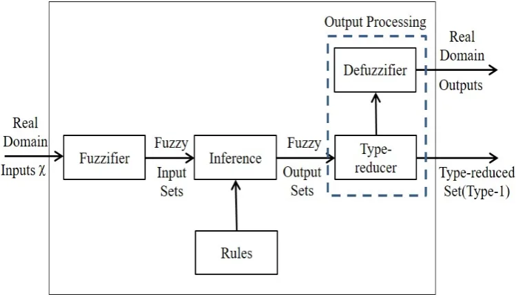
A standard Mamdani-type controller includes a fuzzification module (D/F), an inference module (oR), and a defuzzification module (F/D); two additional modules, namely, the scale factor module and the proportion factor module, are required to convert the data from measurement into data that can be identified by the controller. The Fuzzifier converts the crisp inputs into its membership values for fuzzy sets, the Inference Engine uses the fuzzy rules in the Rule Base to produce fuzzy conclusions, and the Defuzzifier converts these conclusions into crisp outputs. According to Chen (2001), Tshe fuzzification is defining a map from the natural domain of discourse of the inputs and outputs to the fuzzy domain of discourse by giving the scale factors accordingly to represent the experience from experts for the inputs and outputs to ‘translate’ (fuzzify) the natural domain to fuzzy domain, which is easy to ‘re-translate’ (defuzzify) reversely.
Fuzzification Module
The fuzzifier maps the crisp input into a fuzzy set (Karnik, 1999). For fuzzy logic systems, it is important to choose the appropriate method to crisp the human expertise and knowledge and construct the fuzzy sets, and the output is not unique. With the development of science and technology, various mathematical methods have been developed and applied to the fuzzification procedure. In this context, the main issue is choosing a method that is appropriate for obtaining the optimal control output. Additionally, the fuzzy inference engine determines the judgment and output of the fuzzy controller directly. For the purposes of this research, the fuzzy inference plays a very important role in controller design. The controller would be much less popular without a well-designed rule base and fuzzy inference.
* * *
min max min max
0 ( 0 )
2 2
x x x x
x k x
(2.3.21)
where k is the scale factor and is obtained from:
max min
min max
* *
x x
k
x x
(2.3.22)
Suppose the inputs arex X , y Y and the output is z Z , where , ,X Y Z are respectively the fuzzy domain of discourse representing x, y and z. The rules in the rule base have the general expression:
where i[1, ]m ; j[1, ]n ;k[1, ]o and p[1, ]q ; Xi, Yj andZk are the defined membership functions for x, y and z, respectively, and p denotes the number of rules. Here, Xi and Yj are defined as antecedent membership functions while Zk is defined as the consequent membership function, so that the results of rule inferences will be fuzzy.
Rules Inference Module
The fuzzy control rule base is generated from language, either in a series of propositions “if… then …”, or in a control rule table. For a 2-D Mamdani-type controller, the if-then rule always takes the following form:
Rule p: if x is Xiand y is Yj, then z is Zk
After the construction of the rules, the rules composition principles are triggered accordingly.
The coefficient used to transfer the fuzzy domain of discourse to physical domain of discourse is called proportion factor, denoted as ku.
Defuzzification Module
The fuzzy results must be subjected to defuzzification as they cannot be used directly as system inputs. As previously mentioned, defuzzification can be achieved through several methods: the centroid method, maximum of membership method, bisector method, etc.
Therefore, the design procedure of the Mamdani fuzzy control system consists of the following steps:
Determine the natural domain of discourse for inputs and outputs Determine scale factors and obtain the fuzzy domain
Determine inference engine (language base and fuzzy rules base). Determine defuzzification method and obtain the distinct data. Connect the controller output to the system.
2.3.4 T-S Type Fuzzy Control
Consider a fuzzy proposition as: If x1 is A1 and x2 is A2 , then u is U . For this proposition, if we further know that x1 is *
1
A and x2 is * 2
A , then we can infer the new proposition that u is U* .
Again, considering a linear system that can be controlled piecewise, the stated inference can be modified as: “If x1 is A1 and x2 is A2, then u f x x( , )1 2 ”, where output u is a numerical function related to the actuation of the inputs x1 and x2 (without defuzzification), while A1 and A2 are fuzzy sets.
1) Commonly used T-S type fuzzy control:
There are two applications of T-S fuzzy control:
0-order T-S type fuzzy controls: If x1 is A1 and x2 is A2, then u k
1-order T-S type fuzzy control: If x1 is A1 and x2 is A2, then u px1qx2r
Where k, p, q and r are constants.
When using n T-S fuzzy rules to describe a system, suppose the input is xi , it is impossible to correlate with only one rule but several rules. Therefore, suppose the
th
i rule is denoted as Ri
, then:
i
R : If x1 is 1 i
A and x2 is 2 i
A , then uiki (i1 2, , ,K n ) (for 0-order)
Or: Ri : If x1 is 1 i
A and x2 is 2 i
2) Algorithms to obtain output u
Weighted Summation (wtsum):
1 1 2 2 1
m
i i n m
i
U w u w u w u w u
L(2.3.23)
where w denotes the weight of the rule in the total output.
Weighted Average (wtaver):
1 1 1 2 2
1 2
1 m
i i
i n m
m
n i
i w u
w u w u w u
U
w w w
w
L L
(2.3.24)
The typical T-S fuzzy control diagram is shown as follows:
Figure 2-6 T-S Type Control Block Diagram
fuzzy set is that its membership is not clear number or boundaries, but it is derived from another series of membership functions. First introduced by Zadeh in 1975, the type-2 fuzzy set has enabled computers to effectively deal with both linguistic and numerical uncertainty. Since then, there has been a proliferation of studies on type-2 fuzzy sets. Liang and Mendel (1999) were the first to introduce type-2 TSK fuzzy models, outlining the difference between those models and the Mamdani fuzzy model. Consequently, Karnil and Mendel (2001) introduced the operations on type-2 fuzzy sets and Mendel (2002) provided an overview of type-2 fuzzy control. Since the emergence of fuzzy control, it has been used in many applications, such as robots (Lu and Liu, 2016), water tank level control (Galluzzo and Cosenza, 2011), decision-making (Naim and Hagras, 2012) and database design (Niewiadomski, 2010). According to Li et al (2008, 2009), there are also several methods to realize the 3-D type of control. They use three levels of fuzzy sets, which is also called type-3 fuzzy control. However, most of them are firstly using the first (primary) level of set to create the model of the plant. It is very efficiency indeed, to facilitate the consequent fuzzy control systems design process. As it is well known that fuzzy control is very customized type rather than a universal type for design, such fuzzy control system design can be only applied to that plant and cannot be generalized from the very beginning. Secondly, the establishment the three levels of fuzzy sets is usually adopted three different dimensions independently, which cannot efficiently exhibit the link between different levels of dimensions (or, variables). Type-2 fuzzy sets shows clearly the relationship and the influence that the secondary fuzzy sets to the primary fuzzy sets.
decoupled interval type-2 fuzzy sliding-mode controller for controlling the chaos in systems and obtaining a better control performance. Wang and Li (2008) presented fuzzy modelling of dynamic systems with measurement noise. Abbadi et al. (2013) developed an interval type-2 T-S fuzzy controller for non-linear voltage. The proposed controller has been applied to two-generator infinite bus power system. Apart from engineering applications, the type-2 fuzzy control is also used in other areas, such as in exchange rate modelling and prediction (Medina, 2006), and in ATM networks via type-2 fuzzy logic systems (Liang, 2000).
Figure 2-7 The Structure of Type-2 fuzzy control
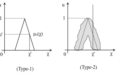
Footprint of Uncertainty
a certain curve but covers a range of space. The space is determined by secondary membership function while correspondingly A( )x is called main membership function. Consequently, the shadow shown in (b) can also be considered as the possible position or footprint of the membership. Therefore, a type-2 fuzzy set is defined mathematically as follows:
Figure 2-8 Comparison of Type-1 and Type-2 Membership Functions (© 2006 IEEE reprinted from Mendel et. al, 2006, Fig. 1. (a) Type-1 MF. (b) Blurred type-1 MF.)
Therefore, a type-2 fuzzy set is defined mathematically as follows:
(( , ), A( , )) , x [0,1]
A% x u % x u x X u J (2.3.25)
Where A% denotes a type-2 fuzzy set, the main membership is 0A%( ) 1x , and the
secondary membership is 0A%( , ) 1x u . If the value of every secondary
Apart from the fact that they rely on type-2 fuzzy sets, type-2 fuzzy rules are similar to type-1 fuzzy rules in terms of the “if-then” structure.
Interval Type-2 Fuzzy Relationship
Define U V, as two domain of discourses, and °(F U V ) denotes the sum of all interval