Supported by the Ministry of Agriculture of the Czech Republic, Project No. 1G58095 and partly supported by the Ministry of Education, Youth and Sports of the Czech Republic, Project No. MSM 6046070901.
Estimation of the Soil Water Retention Curve (SWRC)
Using Pedotransfer Functions (PTFs)
Svatopluk Matula, Markéta MojRová and Kamila ŠpongRová
Department of Soil Science and geology, Faculty of agrobiology, Food and natural
Resources, Czech university of life Sciences in prague, prague, Czech Republic
Abstract: Soil hydraulic characteristics, especially the soil water retention curve and hydraulic conductivity, are essential for many agricultural, environmental, and engineering applications. Their measurement is time-consuming and thus costly. Hence, many researchers focused on methods enabling their indirect estimation. In this paper, Wösten’s continuous pedotransfer functions were applied to the data from a selected locality in the Czech Republic, Tišice. The available data set related to this locality consists of 140 measured soil water retention curves, and the information about the soil texture, bulk density ρd, and organic matter content determined at the same time. Own continuous pedotransfer functions were derived, following the methodology used in continuous pedotransfer functions. Two types of fitting, 4-parameters and 3-parameters, were tested. In 4-parameter fitting, all parameters of the van Genuchten’s equation, θs, θr, α, n, were optimized; in 3-parameter fitting, only three parameters, θr, α, n, were optimised while the measured value of θswas set as constant. Based on the results, it can be concluded that the general equations of Wösten’s pedotransfer functions are not very suitable to estimate the soil water retention curves for the locality Tišice in the Czech Republic. However, the parameters of the same Wösten’s equations, which were calculated only from the data for each particular locality, performed much better. The estimates can be improved if the value for the saturated soil water content θsis known, applied and not optimised (the case of 3-parameter fitting). It can be advantageous to estimate SWRC for a locality with no data available, using PTFs and the available basic soil properties. In addition, to measure some retention curves and/or some their parameters, like θs, can improve the accuracy of the SWRC estimation.
Keywords: continuous pedotransfer function; soil water retention curve; fitting; parametric method; neural network
Soil hydraulic characteristics, like the soil water retention curve and hydraulic conductivity, are indispensable input data for the simulation in agriculture, landscape management, and water-re-sources engineering and all possible environmental incidences of assorted fields. However, the direct measurement is troublesome, time-consuming and expensive. Alternative approaches called pe-dotransfer functions (PTFs) for the predictions of
PTFs . The set consists of 140 measured retention curves (Matula 1988; Kuráž 1989).
A comparison of different approaches to the development of pedotransfer functions for SWRC was presented by Minasny et al. (1999). They divided PTFs into 3 types:
Point estimation – certain points can be esti-mated of the soil water retention curve (for ex-ample for –10, –33 = field capacity, –1500 kPa = permanent wilting point).
Parametric estimation – the relationship of the volumetric soil water content θ and pressure head h
is described by closed-form equation (Brooks & Corey 1964; van Genuchten 1980).
Physico-empirical models – the retention curve is derived from physical attributes.
Three different methods were used to fit the soil wa-ter retention curve PTFs (Minasny et al. 1999): Multiple Linear Regression (MLR)
Extended Nonlinear Regression (ENR) Artificial Neural Network (ANN)
Cornelis et al. (2001) also divided the PTFs into three groups:
Group 1 – application of MLR (Gupta & Larson 1979; Rawls & Brakensiek 1982; Saxton et al.
1986; Šútor & Štekauerová 2000) and ANN (Pachepsky et al. 1996).
Group 2 – application of close-form analytical equation (for example Brooks & Corey 1964 or van Genuchten 1980) was used by Rawls and Brakensiek (1985); together with MLR (Vereeck-en et al. 1989; Scheinhost et al. 1997; Wösten
et al. 1998; Minasny et al. 1999; Wösten et al.
1999) or ANN (Pachepsky et al. 1996; Minasny
et al. 1999; Schaap et al. 1998a, b, 1999).
Group 3 – physico-conceptual approach of the water retention phenomenon (Arya & Paris 1981; Haverkamp & Parlange 1986) and the use of fractal mathematics and scaled similarities (Tyler & Wheatcraft 1989; Comegna et al. 1998).
A large and detailed overview of the status of PTFs was done by Wösten et al. (2001). Nemes
et al. (2003) published an interesting functional evaluation of PTFs derived from different scales of data sets. They worked in three scales: national (Hungarian data), continental (HYPRES data), and intercontinental (US and European data) scales.
[image:2.595.67.532.495.750.2]Wösten et al. (1998) derived either Class PTFs, based on 11 texture/pedological classes, or Con-tinuous PTFs to get θr, θs, α, n soil hydrophysical parameters in both cases. The HYPRES database of hydraulic properties of European soils was created. The works of Wösten et al. (1998) and Matula and Špongrová (2007) were widely used in this study.
Table 1. The borrow pits and undisturbed soil samples (Matula 1988)
Borrow pit Depth (cm) Number of samples
Permanent meadow K1
20 20
50 20
70 4
120 4
Permanent meadow K2
20 20
50 20
100 3
130 3
Permanent grass (close to meteorological station) K3
20 20
40 20
70 3
90 3
MATERIALS AND METHODS
Our objective in this study was to apply the model of Continuous PTFs (Wösten et al. 1998) to the selected locality with sufficient sets of measured water retention data, then to develop the local model coefficients and to evaluate the accuracy of the prediction. The data sets were collected at the locality Tišice, north of Prague, Central Bohemia, the Czech Republic. The soil in this locality is Chernozem (CH in WRB: IUSS/FAO/ISRIC Soil Classification).
Three borrow pits (K1, K2, K3) were dug out and 140 undisturbed soil samples (Kopecký’s ring 100cm3) were taken. Table 1 shows the sampling.
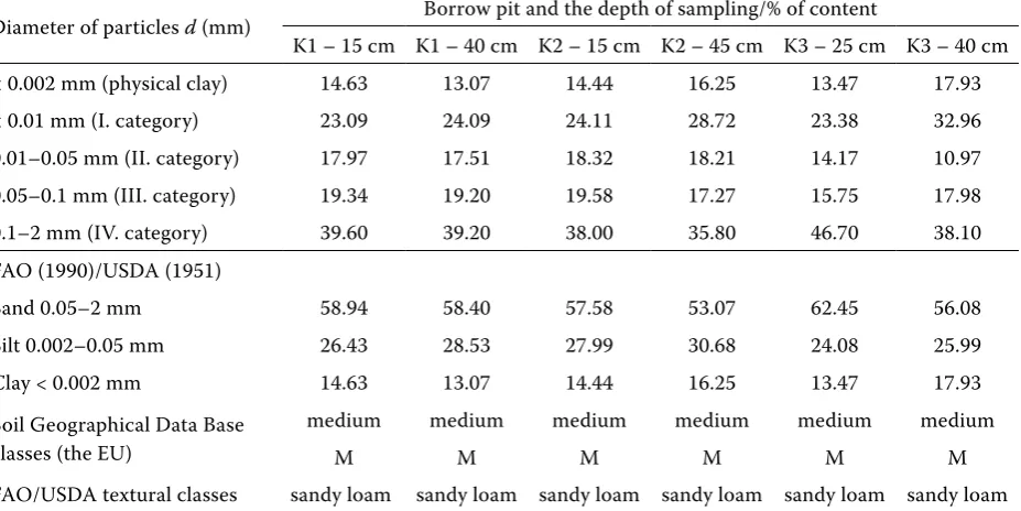
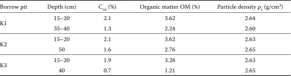
The soil water retention curves measured were carefully evaluated and other important physical soil parameters (particle size distribution analysis results in Table 2, organic matter contents, soil particle densities in Table 3, and dry bulk densities in Table 4) were added. The particle-size analysis was carried out using the standard procedure, i.e. sieving and sedimentation analysis based on Stokes’ Law (hydrometer method). A water pycnometer was employed to find the soil particle density ρz. The organic matter content was measured as the Cox in %. These values were converted into the organic matter in percentage using the conversion equation OM = 1.724 Cox (%).
Those soil samples, taken from the depth below 50 cm, were not used in the PTFs calculations of the final experimental data set of 121 data units.
The inputs for the calculations of the PTFs were:
Contents of clay and silt after FAO system (%) Dry bulk density ρd(g/cm3)
Organic matter OM fraction (%)
Qualitative parameter 1 or 0 for topsoil or subsoil, respectively
The parameterisation procedure was used and the soil water retention curves were fitted by the well known van Genuchten’s equation:
θe(h) = θr (θs – θr) h < 0 (1)
(
1 + (α h)n)
1–1/nwhere:
θe(h) – effective soil water content as a function of pres-sure head
θe(h) = (θ – θs)/(θs – θr) (2)
θs – saturated soil water content – parameter (m3/m3)
θr – residual soil water content – parameter (m3/m3)
θ – actual soil water content (m3/m3)
α, n – empirical parameters
The computer code RETC (van Genuchten et al. 1991) was employed in order to optimise θr,
[image:3.595.68.532.524.756.2]θs, α, n parameters applying two different systems of fitting; 4-parameter fitting (represents fitting
Table 2. Soil texture classes in different classifications
Diameter of particles d (mm) Borrow pit and the depth of sampling/% of content
K1 – 15 cm K1 – 40 cm K2 – 15 cm K2 – 45 cm K3 – 25 cm K3 – 40 cm
< 0.002 mm (physical clay) 14.63 13.07 14.44 16.25 13.47 17.93
< 0.01 mm (I. category) 23.09 24.09 24.11 28.72 23.38 32.96
0.01–0.05 mm (II. category) 17.97 17.51 18.32 18.21 14.17 10.97
0.05–0.1 mm (III. category) 19.34 19.20 19.58 17.27 15.75 17.98
0.1–2 mm (IV. category) 39.60 39.20 38.00 35.80 46.70 38.10
FAO (1990)/USDA (1951)
Sand 0.05–2 mm 58.94 58.40 57.58 53.07 62.45 56.08
Silt 0.002–0.05 mm 26.43 28.53 27.99 30.68 24.08 25.99
Clay < 0.002 mm 14.63 13.07 14.44 16.25 13.47 17.93
Soil Geographical Data Base classes (the EU)
medium medium medium medium medium medium
M M M M M M
of all four parameters), and 3-parameter fitting (represents fitting of three parameters, leaving out θs, which is given as a constant value, taken from the measurement). In the RETC code, the Artificial Neural Network (ANN) is implemented as the code ROSETTA Lite v. 1.0. This code was used to calculate the initial estimates for the re-spective parameters. These parameters were ap-plied into the RETC code for the calculation of the SWRC model parameters. Then, the results of RETC were used as the input data in the software
STATISTICA CZ to derive the coefficients of the PTFs. Continuous PTFs of Wösten et al. (1998) presented in Table 5 were tested as first. In this case, a different 3-parameter fitting was applied, the parameters θs, α, n were optimised, while the parameter θr was fixed at the value of 0.01 follow-ing the Wösten’s methodology.
[image:4.595.64.532.106.229.2]The statistical software package STATISTICA CZ v. 7.0 was the tool for the calculations of the coefficients of the Continuous PTFs in the case of the own parameter calculations. In the case of
Table 3. Values of Cox, organic matter content OM, and soil particle density ρz
Borrow pit Depth (cm) Cox (%) Organic matter OM (%) Particle density ρz (g/cm3)
K1 15–20 2.1 3.62 2.64
35–40 1.3 2.24 2.60
K2 15–20 2.1 3.62 2.63
50 1.6 2.76 2.65
K3 15–20 1.9 3.28 2.63
[image:4.595.65.534.274.354.2]40 0.7 1.21 2.65
Table 4. Basic statistics for dry bulk densities ρd determined in each individual sample from borrow pits K1, K2, K3
Number of
samples (g/cmMean 3) Median (g/cm3) (g/cmMode 3) Frequency of mode Minimum (g/cm3) Maximum (g/cm3)
Borrow pit K1 41 1.48 1.49 1.50 4 1.32 1.65
Borrow pit K2 40 1.57 1.58 1.66 4 1.41 1.74
Borrow pit K3 40 1.45 1.46 1.38 5 1.33 1.59
Table 5. Continuous pedotransfer functions (according to Wösten et al. 1998)
Model parameters of van Genuchten’s equation
θs = 0.7919 + 0.001691 C – 0.29619 D – 0.000001491 S2 + 0.0000821 OM2 + 0.02427 C–1 + 0.01113 S–1 +
0.01472 ln(S) – 0.0000733 OM C – 0.000619 D C – 0.001183 D OM – 0.0001664 topsoil S
α* = –14.96 + 0.03135 C + 0.0351 S + 0.646 OM + 15.29 D – 0.192 topsoil – 4.671 D2 – 0.000781 C2 –
0.00687 OM2 + 0.0449 OM–1 + 0.0663 ln(S) + 0.1482 ln(OM) – 0.04546 D S – 0.4852 D OM + 0.00673 topsoil C n* = –25.23 – 0.02195 C + 0.0074 S – 0.1940 OM + 45.5 D – 7.24 D2 + 0.0003658 C2 + 0.002885 OM –
12.81 D–1 – 0.1524 S–1 – 0.01958 OM–1 – 0.2876 ln(S) – 0.0709 ln(OM) – 44.6 ln(D) – 0.02264 D C
+ 0.0896 D OM + 0.00718 topsoil C
θs –model parameter (m3/m3); α*, n* – transformed model parameters (α* = ln (α); n* = ln (n – 1)); C – content of clay (%);
the own parameter calculations, two methods for the coefficient calculation were selected:
Independent calculation for each borrow pit (K1, K2, K3) for 3- and 4-parameter fittings;
Calculation of the parameters using the data from all borrow pits together also for 3- and 4-para- meter fittings.
In all cases, the estimated points (being equiva-lent to the data measured) of the retention curves expressed as pF were calculated by the application of the own and Wösten’s PTFs.
RESULTS AND DISCUSSION
This study elaborates 121 data units collected from three borrow pits (K1, K2, K3) in Tišice (Matula 1988; Kuráž 1989). The structure of PTFs calculations is schematically presented in Figure 1. The result of the calculations gives 8 sets, 4 equations each, that represent 32 own Continuous PTFs. The equations were devel-oped for the data of all pits together and for each borrow pit locally (K1, K2, K3). The
cor-Total number of calculated pF curves: 472 118 × 9
D
n
4-parameter D
n
3-parameter Tr
6K = K1 + K2 + K3
Tr
40 × 9
D
n
3-parameter Tr 40 × 9
118 × 9 n
4-parameter
Ts
Ts K3
Tr
3-parameter Tr
D
37 × 9
D
n
41 × 9
41 × 9
37 × 9
Tr D
n
4-parameter
Ts
K2
Tr D
n
Borrow pit Fitting Calculated parameters from own continuous PTFs
K1
4-parameter
3-parametr
Ts
Calculated points of retention curves from own continuous PTFs
Tr D
[image:5.595.116.488.249.723.2]n
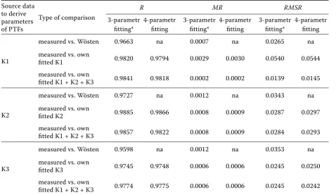
relation coefficients (R), mean residuals (MR), and root mean squared residuals (RMSR) were calculated. Based on MR, the systematic errors between the measured and estimated points of the PF curves were evaluated. The accuracy of the estimates was characterised by RMSR. The correlation coefficient is not powerful enough to represent the goodness of the fit, and thus all the curves measured and estimated were graphically
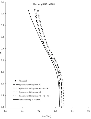
compared. An example of the results obtained with K2 borrow pit is given in Figures 2–4. The accuracy of estimates represented by R, MR, and
RMSR is shown in Table 6.
CONCLUSIONS
[image:6.595.119.492.235.722.2]The data set from the locality Tišice gave us the opportunity to evaluate two types of fitting (3- and
Figure 2. Example of typical comparison of measured and estimated pF curves by using different types of own fittings, Wösten’s fitting and measured SWRC data (rk208 = No. of sample)
Borrow pit K2 – rk208
0.0 0.5 1.0 1.5 2.0 2.5 3.0 3.5 4.0 4.5
0.0 0.1 0.2 0.3 0.4 0.5
T (m3/m3)
pF
Measured
0 0.3 0.6
0 0.3 0.6
Όȱ(m3/m3)ȱȱestimationȱbyȱWösten
Όȱ
(m
3 /m 3 )ȱȱ
m
ea
su
re
d
0 0.3 0.6
0 0.3 0.6
Όȱ(m3/m3)ȱȱestimationȱK2ȱ(3Ȭparameterȱfitting)
Όȱ
(m
3 /m 3 )ȱȱ
m
ea
su
re
d
0 0.3 0.6
0 0.3 0.6
Ό (m3/m3) estimation K1 + K2 + K3 (3-parameter fitting)
Ό
(m
3/m 3)
m
ea
su
re
d
0 0.3 0.6
0 0.3 0.6
Όȱ(m3/m3)ȱȱestimationȱK2ȱ(4Ȭparameterȱfitting)
Όȱ
(m
3/m 3)ȱȱ
m
ea
su
re
d
0 0.3 0.6
0 0.3 0.6
Ό (m3/m3) estimation K1 + K2 + K3
(4-parameter fitting)
Ό
(m
3/m 3)
m
ea
su
re
[image:7.595.66.534.74.733.2]d
[image:7.595.314.524.89.275.2]Figure 3. Example of the results of comparison of 3-para-meter fittings in the selected borrow pit K2
4-parameter fittings). A relatively large data set (121 carefully measured retention curves) and pre-cisely and well measured basic soil physical proper-ties were available. All data were collected during the same time period, using identical methodology performed by a single team of researchers. This offered us a reliable data set, which is unique with respect to both a sufficient volume and homogene-ity. The soil type, Chernozem, is well known for its good soil physical behaviour. Based on the results presented above, we can formulate the following conclusions:
– Continuous PTFs of Wösten et al. (1998) provide quite acceptable estimates for the selected locality Tišice, in spite of the use of Wösten’s parameters derived for a different set of the soil data. In addition, a fixed value for the residual water content (θr), 0.01, was used if no measured data were available.
– The OwnContinuous PTFs gave good estimates of the retention curves. This is documented by very high correlation coefficients, and low RMSR
values (see Table 6).
– The comparison of 3- and 4-parameter fit-tings showed clearly in a majority of cases better results in 3-parameter fitting if the measured θs was introduced into the calculation as the fixed parameter. This θs is quite often available from the basic physical properties determination in common soil survey.
– The authors realise that the above stated con-clusions are based only on one soil type with a very good soil physical behaviour.
The application of the PTFs on the localities with no retention curve data measured is possible, but the estimates can be expressively improved if some retention curves are additionally measured.
The estimates may be sufficiently accurate for many purposes, such as hydrological models, land-scape and watershed management, etc.
[image:8.595.62.541.102.379.2]Acknowledgements. The authors thank Assoc. Prof. Dr. Václav Kuráž for his support with some data of Tišice, and Prof. Dr. Luboš Borůvka for the consultancy con-cerning the use of STATISTICA software package. Table 6. Evaluation of the goodness of fit, R, MR, RMSR values
Source data to derive parameters of PTFs
Type of comparison
R MR RMSR
3-parametr fitting*
4-parametr fitting
3-parametr fitting*
4-parametr fitting
3-parametr fitting*
4-parametr fitting
K1
measured vs. Wösten 0.9663 na 0.0007 na 0.0265 na
measured vs. own
fitted K1 0.9820 0.9794 0.0029 0.0030 0.0540 0.0544
measured vs. own
fitted K1 + K2 + K3 0.9841 0.9818 0.0002 0.0002 0.0139 0.0145
K2
measured vs. Wösten 0.9727 na 0.0012 na 0.0343 na
measured vs. own
fitted K2 0.9885 0.9866 0.0008 0.0009 0.0287 0.0297
measured vs. own
fitted K1 + K2 + K3 0.9857 0.9822 0.0008 0.0009 0.0284 0.0293
K3
measured vs. Wösten 0.9598 na 0.0012 na 0.0353 na
measured vs. own
fitted K3 0.9745 0.9748 0.0006 0.0006 0.0245 0.0250
measured vs. own
fitted K1 + K2 + K3 0.9774 0.9775 0.0006 0.0006 0.0245 0.0242
*There are two types of 3-parameter fitting: in Wösten’s comparison θs, α, n were fitted, θr was equal 0.01, while for the own PTFs parameters θr, α, n were fitted and θs was taken from the measurement
References
Arya L.M., Paris J.F.
(
1981): A physico-empirical model to predict the soil moisture characteristic from partic-le-size distribution and bulk density data. Soil Science Society of America Journal, 45: 1023–1030.Brooks R.H., Corey A.T. (1964): Hydraulic properties of porous media. Hydrology Paper No. 3, Colorado State University, Fort Collins.
Comegna V., Damiani P., Somella A. (1998): Use of a fractal model for determining soil water retention curves. Geoderma, 85: 307–323.
Cornelis W.M., Ronsyn J., Van Meirvenne M., Hart-mann R. (2001): Evaluation of pedotransfer functions for predicting the soil moisture retention curve. Soil Science Society of America Journal, 45: 1023–1030. Gupta S.C., Larson W.E. (1979): Estimating soil water
retention characteristics from particle size distribu-tion, organic matter percent and bulk density. Water Resources Research, 15: 1633–1635.
Haverkamp R., Parlange J.Y.
(
1986): Predicting the soil water retention curve from particle-size distribution:1. Sandy soils without organic matter. Soil Science, 142: 325–339.Kuráž V. (1989): Pedologický průzkum výzkumné plochy na stanici v Tišicích, Katedra hydromeliorací, Fakulta stavební, ČVUT, Praha.
Matula S. (1988): Experimental research on spatial vari-ability, stationary measurements of the characteristics and their computer evaluation. Report of the CTU, Faculty of Civil Engineering, Prague. (in Czech) Matula S., Špongrová K. (2007): Pedotransfer
func-tion applicafunc-tion for estimafunc-tion of soil hydrophysical properties using parametric methods. Plant, Soil and Environment, 53: 149–157.
Minasny B., McBratney A.B., Bristow K.L. (1999): Comparison of different approaches to the development of pedotransfer functions for water retention curves. Geoderma, 93: 225–253.
Nemes A., Schaap M.G., Wösten J.H.M. (2003): Fun-ctional Evaluation of Pedotransfer Functions Derived from Different Scales of Data Collection. Soil Science Society of America Journal, 67: 1093–1102.
Pachepsky Y.A., Timlin D., Varallyay G.
(
1996): Arti-ficial neural networks to estimate soil water retention from easily measurable data. Soil Science Society of America Journal, 60: 727–733.Rawls W.J., Brakensiek D.L. (1982): Estimating soil water retention from soil properties. Journal of Irrigation and Drainage Division ASCE, 108: 166–171.
Rawls W.J., Brakensiek D.L. (1985): Prediction of soil water properties for hydrologic modeling. In: Jones
E., Ward T.J. (eds): Watershed Management in the Eighties. Proc. Symposium of Irrigation and Drainage Division ASCE, April 30–May 1, 1985, Denver, ASCE, New York.
Saxton K.E. et al. (1986): Estimating generalized soil-water characteristics from texture. Soil Science Society of America Journal, 50: 1031–1036.
Schaap M.G., Leij F.J., van Genuchten M.Th. (1998a): Using neural networks to predict soil water retention and soil hydraulic conductivity. Soil Tillage Research,
47: 37–452.
Schaap M.G., Leij F.J., van Genuchten M.Th. (1998b): Neural network analysis for hierarchical prediction of soil hydraulic properties. Soil Science Society of America Journal, 62: 847–855.
Schaap M.G., Leij F.J., van Genuchten M.Th. (1999): A bootstrap neural network approach to predict soil hydraulic parameters. In: Van Genuchten M.Th. et al. (eds): Proc. Int. Workshop on Characterization and Measurements of the Hydraulic Properties of Unsatu-rated Porous Media, October 22–24, 1997,University of California, Riverside.
Scheinost A.C., Sinowski W., Auerswald K. (1997): Regionalization of soil water retention curves in a highly variable soilscape: I. Developing a new pedotransfer function. Geoderma, 78: 129–143.
Šútor J., Štekauerová V. (2000): Hydrophysical Charac-teristics of Soils from Žitný ostrov. Institute of Hydrology SAS, Bratislava. (in Slovak)
Tyler S.W., Wheatcraft S.W. (1989): Application of fractal mathematics to soil water retention esti-mation. Soil Science Society of America Journal, 53: 987–996.
van Genuchten M.Th. (1980): A closed-form equation for predicting the hydraulic conductivity of unsatu-rated soils. Soil Science Society of America Journal,
44: 892–898.
van Genuchten M.Th., Leij F.J., Yates S.R. (1991): The RETC Code for Quantifying the Hydraulic Functions of Unsaturated Soils. US Environmental Protection Agency. Available at http://www.scisoftware.com/pro-ducts/retc_overview/retc_overview.html. (accessed on 23 Aug. 2007)
Vereecken H., Maes J., Feyen J., Darius P. (1989): Estimating the soil moisture retention characteristic from texture, bulk density, and carbon content. Soil Science, 148: 389–403.
Wösten J.H.M., Lilly A., Nemes A., le Bas C. (1999): Development and use of a database of hydraulic pro-perties of European soils. Geoderma, 90: 169–185. Wösten J.H.M., Pachepsky Y.A., Rawls W.J. (2001):
Pedotransfer functions: Bridging the gap between
avai-lable basic soil data and missing soil hydraulic charac-teristics. Journal of Hydrology, 251: 123–150.
Received for publication August 24, 2007 Accepted after corrections October 15, 2007
Corresponding author: