The effectiveness of energy storage in hybrid vehicles

1 THE EFFECTIVENESS OF ENERGY STORAGE IN HYBRID VEHICLES

Daniel Cole

A thesis submitted in partial fulfilment of the requirement of the University of the West of England, Bristol for the Doctorate of Philosophy

Department of Engineering, Design and Mathematics, Faculty of Environment and Technology, University of the West of England, Bristol

2 Abstract

3

Table of Contents

ABSTRACT 2

LIST OF FIGURES 10

NOMENCLATURE AND ABBREVIATIONS USED 14

DEDICATION 17

ACKNOWLEDGEMENTS 18

TABLE OF CONTENTS 3

CHAPTER 1 19

INTRODUCTION 19

1.1 Background 19

1.1.2 Growth of hybrid vehicle market 19

1.1.3 Global environmental issues and climate change 20

1.1.4 Local environmental issues – air quality 21

1.2. The Cost of Energy and the Spectre of Peak Oil 22

1.3 Political Factors, Economic Issues and Financial Incentives 23

1.3.1 Energy costs - supply and demand 23

1.3.2 Reduced taxation class for low carbon emission vehicles 25

1.3.3 Company car tax saving when using hybrid vehicles 25

1.3.4 Hybrid vehicles in London congestion zone 25

1.3.5 Background Summary 25

1.4 A Brief History of Hybrid Vehicles 26

1.5 Recent Developments in Hybrid Vehicles 26

1.5.1 Widely adopted technology 27

1.5.2 Public transport applications 28

1.5.3 Motorsport applications 29

4

CHAPTER 2 30

AIMS AND OBJECTIVES 30

2.1 Aim 30

2.2 Objectives 30

CHAPTER 3 31

LITERATURE REVIEW 31

3.1 Approaches to Vehicle Modelling 31

Methods considered in this chapter are based on numerical modelling techniques. 31

3.1.1 Forward vs backward looking modelling of vehicles 31

3.1.2 Integration methods 32

3.2 Modelling of Vehicles with Conventional Powertrains 33

3.2.1 Engine modelling 33

3.2.2 Modelling transmission and clutch/ torque convertors 33 3.2.3 Calculating fuel consumption and engine exhaust emissions 35

3.3 Modelling of Electric and Hybrid Electric Vehicles 36

3.3.1 Modelling of electric vehicles (EV) 36

3.3.2 Series hybrid 37

3.3.3 Parallel hybrid configuration 38

3.3.4 Series-parallel hybrid configuration 40

3.3.5 Regenerative braking 41

3.3.6 Safety considerations and vehicle stability under braking conditions 45

3.3.7 Control strategies for hybrid vehicles 46

3.4 Electrical Energy Storage 46

3.4.1. Lead acid batteries 47

3.4.2 Nickel-Cadmium Batteries 50

3.4.3 Nickel Metal Hydride 50

3.4.4 Lithium Ion 51

3.4.5 Battery power density and energy density summary 54

5

3.5 Mechanical Energy Storage 55

3.5.1 Energy storage in elastic materials/ gases 55

3.5.2. Compressed gas storage 57

3.5.3 Kinetic energy storage 59

3.5.4 Flywheel “Windage” 60

3.5.5. Flywheel energy storage in Transport application 61

3.5.6 Gyroscopic effects and vehicle stability 61

3.6 Sources of Power Loss in Vehicles 62

3.6.1 Resistance due to drivetrain friction 62

3.6.2 Aerodynamic resistance 62

3.6.3 Rolling resistance 62

3.7 Comparison of Energy and Power Density for Various Forms of Energy Storage Technology 63

3.8 Total Energy 65

3.9 Realism and Validity of Driving Cycles 66

3.10 Methods Used by Vehicle Manufacturers in Vehicle Type Approval Testing 66

3.10.1. Coast down testing 67

3.10.2 Factors affecting rolling resistance, engine performance, and aerodynamic drag 68

3.11 Exhaust Emissions 69

3.12 Other Possibilities for Improvements in Vehicle Fuel Economy 70

3.12.1 Engine efficiency 70

3.12.2 Improving driver behavior, moving towards automation? 70

3.12.3 Engine Downsizing 71

3.12.4 Weight Reduction 71

3.12.5 Start / stop technology 71

CHAPTER 4 73

DEVELOPMENT OF A VEHICLE SIMULATION TOOL 73

4.1 Introduction and Overview 73

4.1.1 Introduction 73

4.1.2 Overview of simulation development 73

6

4.2 Initial Development Work 77

4.2.1. Calculation of vehicle performance and validation of simulation 77

4.2.2 Discussion of 0-60 and maximum speed results 81

4.3 Development of the Version 1 Simulation (Ver. 1) 83

4.3.1 Simulating Clutch Slip 83

4.3.2 Simulating driver throttle response 84

4.3.3 Simulating gear changes 86

4.3.4 Engine braking 87

4.3.5 Mechanical braking 87

4.3.6 Calculation of energy used 87

4.3.7 Brake specific fuel consumption 88

4.4 Effect of Time Step Length on Simulation Results 90

4.5. Validation of Version 1 Simulation 91

4.5.1 Comparison against published manufacturers’ data 92

4.5.2 An example validation test of vehicle model with respect to fuel consumption (long term trial) 92 4.5.3. Short term validation trial - OBD measurement of fuel consumption on specific real-world journeys

for comparison against simulation 94

4.5.4 Simulated fuel consumption over a recorded journey profile 94

4.6 Incorporating a Hypothetical Regenerative Braking and Energy Storage System into the forward-

looking Simulation 95

4.7 Development of the Backward Looking (Version 2) Simulation 97

4.7.1 Simplified backward looking model with engine efficiency related to vehicle speed 97 4.7.2 Incorporating BSFC into the Backward - looking simulation (Version 3) 97 4.7.3 Incorporating Level of Energy (LOE) / State of Charge (SOC) 99

4.7.4 Brake specific emissions data 102

4.7.5 Incorporating engine start / stop 103

4.7.6 Validation of the Ver. 3 simulation 103

4.7.7 Assumptions used in the backward looking simulation 104

CHAPTER 5 105

RESULTS FOR SIMULATED PARALLEL HYBRID POWERTRAINS

INCORPORATING REGENERATIVE BRAKING AND ENERGY STORAGE 105

5.1. Introduction 105

7

5.1.2 Energy storage systems investigated 105

5.1.3 Electrical energy storage 106

5.2. Vehicle Mass vs Energy Saved from Regenerative Braking 108

5.2.1 Results for NEDC case studies 108

5.2.2 Discussion of simulation results for increased vehicle mass vs possible energy savings 111

5.3. The Effect of Energy Transfer Rate on Energy Saving Potential of a Hypothetical Hybrid System 113

5.3.1 Introduction 113

5.3.2 Discussion of results 116

5.4 The Effect of the Energy Capacity of a System on the Energy Saving Potential of a Hypothetical Hybrid

System 117

5.4.1 Introduction 117

5.4.2 Discussion of results from simulation of energy storage system capacity 119 5.4.3. Summary of maximum theoretical energy savings possible 120

5.5 Summary of Results for Theoretical Energy Savings for Hypothetical Hybrid Vehicles with No Weight

Penalty Due to Regenerative Braking and Energy Storage System (Using NEDC) 121

5.6 Simulation Results Taking Into Account the Mass and Performance of a Hypothetical Parallel Hybrid

Power-Train 122

5.6.1 Citroen C1 simulation results 123

5.6.2 Citroen Xsara simulation results 125

5.6.3 Range Rover simulation results 126

5.6.4 Optare Solo SR simulation results 128

5.6.5 Bus 1 (ADL Enviro 400) simulation results 129

5.6.6 Volvo Coach simulation results 130

5.7 Potential Energy Savings from Engine Stop-Start Technology 132

5.7.1. Start – stop engine technology and human behaviour 133

5.7.2 The effect of driving style on fuel consumption 134

5.8 General Discussion 135

5.8.1 Discussion on the effect of vehicle mass 136

5.8.2 The effect of aerodynamic drag coefficient (Cd) on theoretical energy savings from regenerative

8

CHAPTER 6 140

THE EFFECT OF A HYBRID SYSTEM ON EXHAUST EMISSIONS FROM

BUSES 140

6.1 Introduction 140

6.1.2 Exhaust emissions investigated 140

6.2 Transport Scenarios Included in the Emissions Study 141

6.2.1 Bus 1 with Li-Ion Battery ESS 141

6.2.2 Bus 1 with High speed composite flywheel ESS 144

6.3. Study of emissions from an Optare Solo SR 147

6.3.2 Optare Solo SR with High speed composite flywheel ESS 150

6.3 Summary of results from emissions study 152

6.4 Energy density and energy capacity in relation to LOE or SOC 154

6.5 The effect of passenger payload on possible fuel savings and emissions reductions 156

CHAPTER 7 160

CONCLUSIONS AND RECOMMENDATIONS 160

7.1 Simulation Performance 160

7.2 The Effectiveness of Regenerative Braking and Energy Storage In Hybrid Vehicles 161

7.2.1. Findings from the general study (energy savings) 161

7.3 Recommendations for further work 163

7.3.2 Further applications 163

REFERENCES 165

APPENDIX I : Summary of vehicle data used 179

APPENDIX II: Preliminary simulation work 180

APPENDIX III: NEDC Gear shift regime 183

APPENDIX IV: Results from early simulation work 183

9

APPENDIX VI: Engine torque data used in simulation work forward looking simulation work 186

APPENDIX VII: Example scaled BSFC plot 188

APPENDIX VIII: Engine efficiency vs steady state speed 189

APPENDIX IX: Example plot of NOx vs power 190

APPENDIX X: Flowchart for backward looking simulation 191

APPENDIX XI: Regenerative braking and energy storage algorithm 192

APPENDIX XII: Contribution from stored energy towards traction effort in backward looking model 193

10 List of Figures

Figure 1.1: New car registrations AFVs, 2000 – 2012 (SMMT, New Car CO2 Report, 2013) ... 20 Figure 1.2: Hubbert’s peak oil curve (replotted from Hubbert, 1956). BBLS = Barrels of

oil, 1 Barrel of oil is usually defined as having a capacity of 42 U.S. gallons ... 22 Figure 1.3: Changes in weight, horsepower and fuel economy for light vehicles from 1980

– 2010 (US Energy Information Administration, 2011) ... 23 Figure 1.4: Crude Oil Prices 1947 – 2010 (WTRG, 2016) ... 24 Figure 1.5: The Lohner-Porsche series hybrid (Hybrid Vehicle History website). ... 26 Figure 1.6: Block diagram of the Toyota Prius Parallel Hybrid Power train System (Roper, 2014) ... 27 Figure 1.7a (left): How PPM flywheel Aids performance. Figure 1.7b (right): How thermal energy, normally dissipated during mechanical braking, is conserved and stored using flywheel. No units given as quantitative data not available, Figures reproduced from PPM literature demonstrating general performance trends of system. (Parry People Movers, 2009). ... 29 Figure 3.1: Example of a series hybrid powertrain showing energy flow during traction and

braking, (re-drawn from Bosch, 2011). ... 38 Figure 3.2: Example of parallel hybrid powertrain showing energy flow during traction and

braking (Re-drawn from Bosch, 2011). ... 39 Figure 3.3: Energy flow in a series-parallel (SP-HEV) or power-split hybrid (Re-drawn

from Bosch, 2011) ... 40 Figure 4.1: Plot of v, (vehicle speed) against t (time) for the New European Driving Cycle

(NEDC) (from www.ecotest.eu). ... 75 Figure 4.2: Plot of v (vehicle speed) against t (time) for the Artemis Urban Cycle (Andre,

2004). ... 76 Figure 4.3: The MLTB cycle (TfL 2009) Plot of vehicle speed v (kph) against time t (s) .. 77 Figure 4.4: Forces acting on a vehicle. ... 78 Figure 4.5: Typical approximate vehicle drag coefficients (from:

www.engineeringtoolbox.com 2012). ... 79 Figure 4.6: Simulated acceleration times for different classes of existing conventional

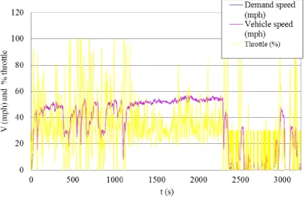
vehicle. ... 81 Figure 4.7: Flow chart of Ver. 1 Simulation with PID control and BSFC incorporated ... 85 Figure 4.8(a) (Top): Gear changes during the simulated Artemis Road cycle for a Citroen

C1 (1.0 l) Chup =3000 rpm Chd = 1500 rpm... 86 Figure 4.8(b) (bottom): Demand speed, vehicle speed and % throttle for the same journey.

... 86 Figure 4.9: An example brake specific fuel consumption plot for a mid- sized car: Saturn

1.9 DOHC petrol engine (ecomodder .com, 2012). ... 89 Figure 4.10: Results from the time step length study over NEDC... 91 Figure 4.11: Results from the time step length study showing all 3 parts of the NEDC ... 91 Figure 4.13: Comparison between simulated (ver.4) and recorded (OBD) instantaneous

11 Figure 4.14: ... 96 RB&ES Flowchart ... 96 Figure 4.18: An example LOE or SOC operating envelope incorporated in Ver. 3

simulation ... 100 Figure. 4.19: Flow chart detailing how SOC is limited to SOCmax in the vehicle model

during braking conditions. ... 101 Figure 4.20: Flow chart detailing how SOC is limited to SOCmin in the vehicle model

acceleration or steady state conditions. ... 101 Figure.4.21 An example NOx emissions map for the Navistar 7.3l Diesel (ADVISOR,

2000) ... 102 Figure.4.22 Comparison between simulation data practical trials conducted for bus 1 .... 103 Figure 4.23: Summary of energy and density values used in the simulation to generate data

in figures Chapter 5. Energy and power density from Cheng et al (2008), motor generator power density from Burke et al (1980) ... 104 Figure 5.1(a): Summary of energy and density values used in the simulation to generate

data in this chapter. Energy and power density from Cheng et al (2008), motor

generator power density from Burke et al (1980) ... 106 Figure 5.1(b) Vehicle types simulated to investigate maximum energy transfer rates

required ... 108 Figure 5.2: Theoretical mass vs energy saving for C1 1.0 (petrol) incorporating a RB&ESS with 50 % efficiency ... 109 Figure 5.3: Theoretical mass vs energy saving for Citroen Xsara 1.4 (petrol) incorporating

a hypothetical RB&ESS with 50 % efficiency ... 110 Figure 5.4: Theoretical mass vs energy saving for Range Rover 5.0 (petrol) incorporating

hypothetical RB & ESS with 50 % efficiency ... 110 Figure 5.5: Theoretical mass vs energy saving for a Volvo B11R Coach incorporating a

hypothetical RB&ESS with 50 % efficiency ... 111 Figure 5.6: Citroen C1 energy saving vs energy transfer rate (standard mass) and

RB&ESS, η = 50% (lwr case k) ... 114 Figure 5.7: Citroen Xsara energy saving against energy transfer rate (Standard mass) .... 114 Figure 5.8: Range Rover 5.0 petrol energy saving against energy transfer rate (standard

mass) ... 115 Figure 5.9: Volvo B11R energy saving against energy transfer rate (standard mass) ... 115 Figure 5.10: Maximum energy transfer rate required to fully utilize recoverable energy

available through regenerative braking for different vehicle types over NEDC ... 116 Figure 5.11: The effect of the energy storage system capacity of the energy saving

potential for a Citroen C1. ... 117 Figure 5.12: The effect of the energy storage system capacity of the energy saving

potential for a Citroen Xsara ... 118 Figure 5.13: The effect of the energy storage system capacity of the energy saving

potential for a Range Rover ... 118 Figure 5.14: The effect of the energy storage system capacity of the energy saving

potential for a Volvo B11R Coach ... 119 Figure 5.15: Energy storage capacity required for a hybrid system to achieve maximum

12 Figure 5.16: Vehicle mass vs maximum potential tractive energy savings from a 50% eff

RB&ESS sys (with no weight increase over standard vehicle mass) for NEDC ... 120 Figure 5.17: Collated results for backward looking NEDC simulation update numbers... 122 Figure 5.18 Key parameters of the hypothetical hybrid system modelled to generate results shown in Figures 5.19 to 5.26 * Hitatchi (2008) **Burke (1980) ... 122 Figure 5.19: C1 % fuel energy saving (comparing to a vehicle with standard mass) vs %

mass increase due to parallel hybrid system with RB&ESS (compared to standard vehicle mass) for NEDC drive cycle. ... 123 Figure 5.20: C1 % fuel energy saving (compared to a vehicle with standard mass) vs %

mass increase due to parallel hybrid system with RB&ESS (compared to standard vehicle mass) for Artemis drive cycle. ... 124 Figure 5.24:Range Rover Sport 5l (petrol) % fuel energy saving (comparing to a vehicle

with standard mass) vs % mass increase due to parallel hybrid system with RB&ESS (compared to standard vehicle mass) for Artemis drive cycles. ... 127 Figure 5.25: Optare Solo SR % fuel saving (comparing to a vehicle with standard mass) vs

% mass increase due to parallel hybrid system with RB&ESS using Li-ion ESS (compared to standard vehicle mass) for MLTB drive cycle. ... 128 Figure 5.26: % fuel saving (comparing to a vehicle with standard mass) vs % mass

increase due to parallel hybrid system with RB&ESS using Li-ion ESS (compared to standard vehicle mass) for MLTB drive. ... 129 Figure 5.27: Volvo B11R Coach, % fuel energy saving (comparing to a vehicle with

standard mass) vs % mass increase due to parallel hybrid system with RB&ESS (compared to standard vehicle mass) for NEDC drive cycles. ... 130 Figure 5.28:Volvo B11R Coach, % fuel energy saving (comparing to a vehicle with

standard mass) vs % mass increase due to parallel hybrid system with RB&ESS (compared to standard vehicle mass) for Artemis drive cycles. ... 131 Figure 5.29: Summary of results from section 5.6 ... 131 Figure 5.30: The simulated energy saving potential of a simulated start – stop engine

system for a range of vehicles on NEDC ... 132 Figure 5.31: The simulated effect of driving style on fuel economy, (mpg / engine speed

for upward gear changes) For 2010Citroen C1 1.0l on combined NEDC ... 135 Figure 5.32: The effect of reduced vehicle mass on fuel energy requirement for Citroen C1 1.0 l on the Artemis Road cycle ... 137 Figure 5.33: The effect of drag coefficient on possible fuel energy savings (shown as a %

of standard vehicle fuel requirement) for the Range Rover sport 5.0l (Cd taken as 0.3 for all other modelling with this vehicle type). ... 138 Figure 6.1: Summary of energy and density values used in the simulation to generate data

in section 6. Energy and power density from Cheng et al (2008), motor generator power density from Burke et al (1980) ... 142 Figure. 6.2: Estimated reductions in NOx with example Li-Ion battery parallel hybrid

system (0%<SOC<100%, SOCinit = 0%) ... 142 Figure. 6.3: Estimated reductions in PM with example Li-Ion battery parallel hybrid

system (0%<SOC<100%, SOCinit = 0%) ... 142 Figure. 6.4: Estimated reductions in NOx with example Li-Ion battery parallel hybrid

13 Figure. 6.5: Estimated reductions in PM with example Li-Ion battery parallel hybrid

system (40%<SOC<80%, SOCinit = 50%) ... 144 Figure. 6.6: Hybrid system power and energy densities used for simulation work in section 6.2.2 ... 145 Figure.6.7: Estimated reductions in NOx with flywheel ESS in parallel hybrid system

(0%<SOC<100%, initial SOC = 0%) ... 145 Figure. 6.8: Estimated reductions in PM with flywheel ESS in parallel hybrid system

(0%<SOC<100%, initial SOC = 0%) ... 146 Figure.6.9: Estimated reductions in NOx with flywheel ESS in parallel hybrid system

(10%<LOE<100%, initial SOC = 50%) ... 147 Figure. 6.10: Estimated reductions in PMxx with flywheel ESS in parallel hybrid system

(10%<SOC<100%, initial SOC = 50%) ... 147 Figure.6.15: Bus 2 Estimated reductions in NOx with flywheel ESS in parallel hybrid

system (0%<SOC<100%, initial SOC = 0%) ... 150 Figure. 6.17: Estimated reductions in NOx with flywheel ESS in parallel hybrid system

(10%<SOC<100%, initial SOC = 50%) ... 151 Figure. 6.18: Estimated reductions in PM with flywheel ESS in parallel hybrid system

(10%<SOC<100%, initial SOC = 50%) ... 152 Figure. 6.19: Summary of results for bus 1 with Li-ion ESS in parallel hybrid system .... 153 Figure. 6.20: Summary of results for bus 1 with Flywheel ESS in parallel hybrid system

... 153 Figure. 6.21: Summary of results for Optare Solo SR with Li-ion ESS in parallel hybrid

system ... 154 Figure. 6.22: Summary of results for Optare Flywheel ESS in parallel hybrid system ... 154 Figure. 6.23: % reduction in NOx (compared to standard) vs Passenger load for Bus 1 ... 157 Figure. 6.24: % reduction in PM (compared to standard) in PM vs Passenger load for Bus 1 ... 157 Figure. 6.25: reduction in fuel consumption (compared to standard) in PM vs Passenger

load for Bus 1 ... 158 Figure. 6.26: Cumulative fuel consumption (hybrid compared to standard) over the MLTB cycle Red = standard vehicle, green = hybrid ... 158 Figure. 6.27: Example LOE plot for bus 1 over the MLTB cycle with no pre-charge and

full passenger load. SOCmin= 10% ... 159 Figure A1: Citroen C1 (1.0l) comparison between simulation and manufacturer’s data .. 183 Figure A2: Mazda MX5 (1.8l) comparison between simulation and manufacturer’s data 184 Figure A3: Range Rover (5.0l) comparison between simulation and manufacturer’s data

14 Nomenclature and abbreviations used

Units

A Maximum cross section area of vehicle m2

a Acceleration m/s2

α Gradient °

Cd Drag coefficient --

Crr Coefficient of rolling resistance --

F Force N

mv Mass of vehicle kg

Faero Aerodynamic drag N

Froll Rolling resistance N

Fgrad Gradient resistance N

Ftract Traction force N

Fbrake Braking force N

Bbrakelim Simulation over-speed constant to trigger braking m/s g Gravitational acceleration = 9.81 m/s2

v Velocity m/s or mph

t Time seconds

𝑣𝑠𝑖𝑚 Simulated velocity m/s

𝑣_𝑑𝑒𝑚 Demand velocity m/s

𝜌 Density of air kg/m3

15

T Torque N.m

𝜂_𝑒𝑛𝑔 Overall engine efficiency --

𝜂_{𝑡𝑟𝑎𝑛𝑠} Transmission efficiency --

DOD Depth of Discharge %

SoC State of Charge %

SoCmin Maximum state of charge % SoCmax Minimum state of charge % SoCinit Initial state of charge %

𝜔_{𝑢𝑝𝑠ℎ𝑖𝑓𝑡} Engine speed for gear change up rpm

𝜔_{𝑑𝑜𝑤𝑛𝑠ℎ𝑖𝑓𝑡} Engine speed for gear change down rpm

𝑣𝑐𝑙𝑢𝑡𝑐ℎ𝑠𝑙𝑖𝑝 Speed below which clutch slip occurs mph

𝐶_𝑃𝐼𝐷 PID Control term --

𝐸𝐵_𝑙𝑖𝑚 Engine braking force limit N

𝐸𝑖𝑑𝑙𝑒

𝐹𝑒𝑛𝑔𝑏𝑟𝑐𝑜𝑛𝑠𝑡 Engine braking constant --

𝐹_{𝑒𝑛𝑔𝑏𝑟} Engine braking force

BSFC Brake specific fuel consumption g/kWhr (g=grams) CVT continuously variable transmission

EPA Environmental protection Agency (US) ECE Economic Commission for Europe ESS Energy storage system

16 ICE internal combustion engine

KESS kinetic energy storage system NEDC New European Drive Cycle LOE Level of Energy

SOC state of charge

RB&ES regenerative braking and energy storage ESP electronic stability program

EV Electric vehicle

HV Hybrid Vehicle

SP-HEV Series-parallel hybrid electric vehicle PM Particulate matter

NOx Nitrogen Oxides

MLTB Millbrook London Transport Bus cycle LowCVP Low Carbon Vehicle Partnership

EMPA Swiss Federal Laboratories for Materials Science and Technology TfL Transport for London

17 Dedication

18 Acknowledgements

I would like to express my thanks to a number of people who helped to make this work possible. In particular I would like to thank Dr. Mike Ackerman, Dr. Vince Coveney and Dr. Matthew Studley for their help, encouragement and guidance throughout this project, I was very fortunate that they agreed to supervise this project. I am also grateful to Dr Terry Davies who was my Director of Studies in the early stages of the project and contributed to defining the research aims. In addition to the supervisory team, Dr. John Kamalu kindly assisted with advice and encouragement.

Throughout this project I have been fortunate to have the encouragement and friendship of my colleague, and fellow part-time research student, Nathan Townsend (MPhil) and I thank him for his help. Thanks are also in order for Przemyslaw Kukian who gave helpful advice and encouragement during his time as a PhD student in the department and who also assisted in collecting validation data. Additional validation data was recorded on test runs kindly driven by Rachel Szadziewska using her own car which was much appreciated. Studying part-time whilst working full time in a busy department has involved plenty of challenges and I would like to thank UWE for supporting me, but especially Nick Tidman and Huw Dobson for giving me the opportunity to study part-time.

I owe a great deal to my Mother and Father, Kath and Graham, along with the rest of my family for their love, encouragement and support throughout my studies and life in general. They have taught me the most important things of all. Finally I would like to thank Jane whose, love, encouragement and patience has been so vital.

The following individuals and organisations have generously made technical and test data available which has been very useful for this project and for planned future work.

Finn Coyle (TfL)

Brian Robinson (LCVP) Phil Hinde (Crossrail)

Thomas Beutler EMPA (Swiss Federal Laboratories for Materials Science and Technology)

19

CHAPTER 1

INTRODUCTION

1.1 Background

Efforts to improve vehicle efficiency and reduce emissions by road transport have increased in recent years for several reasons including increasing awareness of finite oil resources, concerns over greenhouse gas emissions and associated climate change, and impacts on human health. At present 20% of global greenhouse gases are attributed to transport (The Royal Society, 2008) and 74% of oil is used in the manufacture of petrol and diesel for road transport (TRANSform Scotland, 2007). The 700 million vehicles currently in use worldwide is set to rise to 2.5 billion (Chan, 2002). Pressure from governments and consumers has begun to force manufacturers to investigate ways to increase fuel economy of vehicles and lower exhaust emissions, particularly through use of hybrid power train systems. These combine different propulsion and energy storage technologies in an attempt to optimise efficiency. Hybrid power trains can be divided into two broad types: series and parallel, terms which refer to the flow of energy through the system. The basic principle of these two formats is shown in sections 3.3.1 and 3.3.2. Before looking further into the details of hybrid vehicles and the technology employed, background issues relating to transport energy requirements have been considered.

1.1.2 Growth of hybrid vehicle market

20 Figure 1.1: New car registrations AFVs, 2000 – 2012 (replotted from SMMT, New

Car CO2 Report, 2013)

Although drivers may feel they are helping the environment using hybrids, the real situation is rather more complex and vehicles which are comparatively fuel efficient and have low exhaust emissions are, at best, doing less damage to the environment.

1.1.3 Global environmental issues and climate change

It is generally acknowledged that climate change was first suggested by Joseph Fourier (1768-1830) who described how the composition of the earth’s atmosphere could have an effect on climatic conditions (Weart 2013). These early concepts were developed further by Svante Arrhenius (1859-1927) who first proposed the correlation between increased atmospheric CO2 levels from the burning of fossil fuels and increased temperatures. By the late 1980’s the idea of climate change being accelerated by human activity had gained wide acceptance within the scientific community and the wider public. Since that time there has been a great deal of research carried out in the field of climate modelling to predict future climatic conditions (Maslin, 2004).

It is likely that the widespread knowledge and acceptance of climate change has influenced the car buying public and helped to generate interest in vehicles that are fuel efficient and have low emissions. With hybrid vehicle sales increasing annually as shown in Figure 1.1, the affordability of these vehicles has improved with models such as the Toyota Prius (1997 – present(2016)) gaining mainstream status.

0 5000 10000 15000 20000 25000 30000 35000

2000 2002 2004 2006 2008 2010 2012 2014

New

c

ar

r

e

gi

str

ati

on

s

21 1.1.4 Local environmental issues – air quality

Air pollution in conjunction with climatic conditions, caused at least 4000 deaths single night in London during December 1952, and led to the introduction of the Clean Air Act (1956). Globally, the United Nations Environment Programme estimates that urban air pollution is linked to as many as one million premature deaths each year and a further one million pre-natal deaths (UNEP 2013).

The combustion processes of vehicle engines make a significant contribution to air pollution in the form of emissions of carbon monoxide, hydrocarbons, nitrogen oxides (NOx), and particulate matter (PM) (Heywood, 1988), some of which react in the presence of sunlight to produce ozone (O3) (Haagen-Smit, 1952). Many studies have shown links between vehicle emissions and specific health problems, for example Kampa and Castanas (2008) linked PM, NOx, O3 and volatile organic compounds (hydrocarbons) to respiratory and cardiac disease and reduced life expectancy; Gehring et al (2010) established a link between levels of traffic pollution and asthma; Yim and Barrett (2012) estimated that combustion emissions from transport cause approximately 7500 early deaths per year; and a recent review of medical studies has shown that exposure to gaseous and particulate matter pollution - including those emitted by vehicles - increased the immediate risk of stroke (Shah et al, 2015).

Governments have implemented various restrictions on vehicles in attempts to improve air quality and also to reduce congestion which reduces the concentration of emissions. For example California has stringent exhaust emission limits, and a congestion charging zone exists in central London where motorists pay a charge to enter a specified zone.

Despite increasing legislation to limit vehicle exhaust emissions increasing levels of traffic continue to present serious air quality problems. The European Commission has launched infringement proceedings against the UK Government over exceedances of EU PM air quality standards in London, and the current annual urban air pollution limits for NOx and PM were exceeded within the first week of 2016 in areas of central London (Vaughan, 2016).

22 million in 2002 to more than two billion in 2030 (Dargay et al, 2007). The resultant lowering of air quality from vehicle emissions is of particular concern.

1.2. The Cost of Energy and the Spectre of Peak Oil

The term ‘peak oil’ was first used in 1956 by M. King Hubbert a geologist working for the Shell Oil Company. He calculated the future rate of oil extraction and calculated that world-wide oil production would hit a maximum level, as crude oil takes millions of years to form and, therefore it is a non-renewable energy source on human timescales. Figure 1.2 shows the skewed bell shaped curve that he determined.

Figure 1.2: Hubbert’s peak oil curve (replotted from Hubbert, 1956). BBLS = Barrels of oil, 1 Barrel of oil is usually defined as having a capacity of 42 U.S. gallons Although there is a degree of uncertainty over exactly when peak oil has occurred or will occur, more recent forecasts including further oil discoveries and improved extraction technologies, are strikingly similar to Hubbert’s predictions. Energy demands are increasing as the global population rises and living standards improve in developing countries. Along with this is an expectation of car ownership and the associated demand for petrol and diesel (derived from crude oil). In China, for example, the number of civilian vehicles registered has risen from 1.78 million in 1980 to around 78 million in 2010 (NBSC 2012). This represents an approximately 44 fold increase in 30 years.

0 5 10 15

1850 1900 1950 2000 2050 2100 2150 2200

Bill

ions

of

BBL

S

/

Y

r

Year

Hubbert's Peak Oil curve

Proven reserves 250x109 _BBLS

Cumulative production 90x109

23 Improvements in fuel efficiency are increasingly necessary to offset air pollution from greater numbers of road vehicles. In recent years although improvements have been made in fuel economy, these improvements have been relatively modest compared to the marked gains in horsepower, see Figure 1.3 below. 0-60 mph times have steadily fallen, which suggests that improvements in engine efficiency have been partly negated by increases in engine power. A similar trend is apparent in the European market although fuel economy Figures are generally higher for European cars.

Figure 1.3: Changes in weight, horsepower and fuel economy for light vehicles from 1980 – 2010 (replotted from US Energy Information Administration, 2011)

1.3 Political Factors, Economic Issues and Financial Incentives

1.3.1 Energy costs - supply and demand

Despite the rising popularity of electric vehicles the majority of vehicles on the road still rely on petrol or diesel and as overall vehicle numbers rise, the demand for fuel continues to increase. The price of crude oil is largely influenced by demand, however it is also affected by a number of rather complex geopolitical and socio political factors including oil fields becoming exhausted, new sources being discovered, conflicts and changes in political systems and relations between regions. Natural disasters such as tropical storms, floods and tsunamis as well as man-made disasters such as oil spills and platform fires can also affect oil price. Figure 1.4 shows how fuel prices have varied between 1947 and 2010. The effects of events such as revolutions, wars and recessions can be clearly seen.

0 50 100 150 200 250

1980 1985 1990 1995 2000 2005 2010

In

d

ex:

19

80

=1

00

Model year HP

24 Figure 1.4: Crude Oil Prices 1947 – 2010 (replotted from WTRG, 2016)

Fuel prices influence the price of other products partly because many businesses depend on transporting goods large distances by land, sea and air. Within the scope of this research road transport energy requirements are of particular interest. OPEC (Organisation of Petroleum Exporting Countries) play a key role in setting oil prices and the complex details behind how prices are adjusted are beyond the scope of this work. However, increases in fuel efficiency resulting in lower running costs will be attractive to consumers. In addition to the environmental concerns that many motorists have, this is a further incentive for consumers to consider AFVs (alternative fuelled vehicles) including hybrid vehicles that claim, to varying extents, attractive fuel economy along with good performance. The depletion of fossil fuel sources has contributed to increased oil and gas prices and associated increased domestic fuel and transport costs. These financial costs may be most noticeable in the developed world where far more energy is used per head of population than in less developed nations. However, the physical environmental damage is often wrought in the less developed regions where fossil fuels are extracted. The human cost associated with this environmental damage is difficult to quantify.

0.0 20.0 40.0 60.0 80.0 100.0 120.0

1940 1950 1960 1970 1980 1990 2000 2010 2020

20

10

$/Bar

re

l

1947 - 2011 "world price"

U.S. 1st Purchase Price (wellhead)

25 1.3.2 Reduced taxation class for low carbon emission vehicles

Many government taxation policies offer incentives to use low emissions vehicles providing additional financial benefits to users of hybrids. Within the UK, for example, rates of vehicle tax are charged according to manufacturer-registered vehicle emissions of carbon dioxide (CO2). In 2015 new cars that emit less than100g CO2/km are exempt from vehicle tax. Above this emission Figure there is a sliding scale up to a maximum charge of £505 for vehicles emitting 255 g CO2/km and above (UK Government, 2015). The fees are slightly reduced in the case of alternatively fuelled vehicles (AFVs) e.g. £495 maximum charge. This offers a substantial reduction in the fixed annual running costs for both private and fleet users in addition to the possible savings from reduced fuel consumption.

1.3.3 Company car tax saving when using hybrid vehicles

Employees are taxed on the benefit of having a company car, however this tax rises with increased CO2 emissions varying from 0% (of the vehicle’s value) annually for a vehicle with 0g CO2/km at point of use (i.e. electric vehicles), up to 37% for a vehicle with 230g CO2/km or more (Next greencar.com 2015), thus providing an incentive for businesses to provide electric cars for their employees.

1.3.4 Hybrid vehicles in London congestion zone

Vehicles with CO2 emissions below 100g/km were originally exempt from the London congestion charge. The low emissions for hybrids widely reported by manufacturers’ has encouraged businesses and private motorists within the Congestion Zone to purchase low emission vehicles including many hybrids such as the Toyota Prius. The extensions to the scheme made in 2013 reducing the exemption limit from 100 g CO2/km to 75 g CO2/km (Lydall, 2013) caused controversy amongst owners of low emissions vehicles as many lost exemption status.

1.3.5 Background Summary

As shown from the overview in sections 1.1-1.3, two principal challenges exist for future road (and other) vehicles.

(i) Fuel supplies: Dwindling finite supplies of fossil fuels – i.e. oil.

26 Hybrid vehicles and associated technologies present opportunities to address the growing need for improvements in vehicle fuel economy and reduced emissions. Existing road transport examples include a range of cars and some public transport applications. An area requiring further investigation is how possible energy savings vary across a range of transport and journey types.

1.4 A Brief History of Hybrid Vehicles

Over the last 15 years hybrid vehicles (HVs) have been gaining acceptance and popularity. Although they are often considered new technology, it is widely acknowledged that one of the first examples – a series hybrid- was designed and built in 1899 by Dr Ferdinand Porsche (Bergsson, 2005), shown in Figure 1.5. By 1915 parallel hybrids were being produced in small numbers (Modak & Sane, 2006).

27

1.5 Recent Developments in Hybrid Vehicles

1.5.1 Widely adopted technology

Although early examples were relatively basic, modern hybrid vehicles are highly sophisticated, utilising a combined series - parallel approach incorporating power split transmissions and computer control of the energy balance between the ICE and energy storage, such as that used in the Toyota Prius, shown in Figure 1.6 below. An explanation of the key features of series, parallel and series – parallel powertrains is given in sections 3.3.1 and 3.3.2. Features such as regenerative braking are now incorporated whereby the electrical machines used for traction can work as generators to provide braking force and generate electricity which can be stored for use later as required.

Figure 1.6: Block diagram of the Toyota Prius Parallel Hybrid Power train System (redrawn from Roper, 2014)

28 At present, fuel efficiency figures quoted for hybrid vehicles and conventional European vehicles are based on the New European Driving Cycle (NEDC). This cycle includes components representing urban, extra urban and combined driving conditions. All new vehicles are subject to this standard test, although manufacturers often use rolling road tests (factored to take account of resistive forces) to ensure control over all test parameters. Whilst a useful standard for comparison purposes, independent tests and anecdotal evidence from car drivers, suggest that the manufacturer’s quoted mpg figures are rarely attained in practice. An independent test conducted by the US Department of Energy showed a 2010 Toyota Generation III Prius hybrid achieved a combined fuel consumption figure of 44.3mpg (US Dept. of Energy, 2011). Equivalent UK findings of 47 mpg appear to be typical for the 2009 model (RAC, 2009). The figure quoted by Toyota is 65.69 mpg (Toyota, 2010), approximately 39% higher than the US findings.

The variations between quoted and actual fuel efficiency figures can be influenced by several factors such as driver behaviour and methods used in official testing of vehicles (discussed further in 3.12). An in depth investigation of the different factors is outside the scope of this research, however work carried out by Hari et al (2012) showed fuel savings of 7.6% - 12% from driver behaviour alone.

1.5.2 Public transport applications

The application of HV technology is not limited to personal transport. Increasingly, public transport vehicles such as buses are emerging with hybrid power trains.

In 2006 Transport for London (TfL) introduced hybrid buses and by May 2012, 225 diesel-electric hybrid buses were in operation. These buses incorporate regenerative braking and use batteries for on-board energy storage. The environmental benefits claimed include a 30% reduction in fuel use, a minimum 30% reduction in CO2, reduced oxides of nitrogen and carbon monoxide along with lower noise levels (TfL, 2012). Lothian Buses (Scotland) currently run 15 hybrid buses and claim a 30% reduction in fuel consumption and reduced emissions (Lothian Buses, 2012).

29 Figure 1.7a (left): How PPM flywheel Aids performance. Figure 1.7b (right): How thermal energy, normally dissipated during mechanical braking, is conserved and stored using flywheel. No units given as quantitative data not available, Figures reproduced from PPM literature demonstrating general performance trends of

system. (Parry People Movers, 2009).

1.5.3 Motorsport applications

In 2009 regenerative braking was incorporated into Formula one racing. Cars are fitted with motor generator units and energy storage. Early versions of systems used were claimed to provide maximum performance of an additional 60kW of power for 6.7 seconds per lap. For recent developments it is claimed that the system can contribute an extra 120kW for up to 33 seconds per lap (Formula 1.com, 2014). As with other motorsports technologies, investment in hybrid systems is likely to have long term benefits for the wider transport field.

1.5.4 The application of hybrid technology

Much existing research in the field deals with specific aspects of hybrid vehicle technology. As suggested earlier, less attention has been given to the question of where and how it can be used to best effect in terms of energy savings across a wide range of vehicle and journey types.

30

CHAPTER 2

AIMS AND OBJECTIVES

2.1 Aim

The aim of this research is to critically evaluate the overall energy saving effectiveness of regenerative braking and on-board energy storage in hybrid vehicles under a variety of transport scenarios. The scope of vehicle classes investigated ranges from small lightweight vehicles through to large vehicles such as buses and coaches. In the course of this work alternative approaches to energy saving are also considered. The emphasis of the study is to investigate how the energy requirement might be reduced through the use of regenerative braking and energy storage in hybrid power trains, across a broad range of scenarios and to establish where the greatest benefits might be sought. These can then be explored in greater depth to assess potential reductions in exhaust emissions.

2.2 Objectives

(i) Carry out a thorough literature review to evaluate existing work in this field to study existing applications of regenerative braking and energy storage in hybrid vehicles and establish how this work contributes to the field.

(ii) Develop and/or study a simulation tool or tools to predict energy savings across a range of vehicles and journey types.

(iii) Validate and/or compare the simulation tools using data from experimental trials and where necessary refine the simulation tools to give an acceptable level of realism while optimising the simplicity and flexibility of the tool.

(iv) Apply the simulation to investigate energy usage across a wide range of vehicle and journey types with and without regenerative braking and on-board energy storage to compare potential benefits.

(v) Use the results from vehicle energy study to identify across which vehicle classes and journey types the greatest reduction in energy requirement might be achieved. (vi) Having identified where regenerative braking and energy storage might be most usefully employed, study in greater depth the energy efficiency improvements and reduction in emissions that might be made within these transport scenarios -including consideration of alternative approaches for energy saving.

31

CHAPTER 3

LITERATURE REVIEW

Before developing the simulation tool and generating results, relevant literature regarding approaches to modelling vehicle performance, vehicle energy efficiency, hybrid vehicles, regenerative braking, energy storage systems and associated technologies was studied. This enabled the author to evaluate research that has been carried out by others and study existing systems, technology and findings.

3.1 Approaches to Vehicle Modelling

Methods considered in this chapter are based on numerical modelling techniques. 3.1.1 Forward vs backward looking modelling of vehicles

(i) Forward looking simulation

In forward looking simulations driver response to a demand condition is modelled. At any given moment the output (road speed) is compared with the demand and the driver model sets the throttle position or braking effort accordingly. The throttle position output from the driver model is used in the engine model to determine engine torque. The torque data is then used in the transmission part of the vehicle model where transmission ratio and efficiency are taken into account such that output torque at the driving wheels and corresponding tractive force, and therefore acceleration, can be found. In the case of braking conditions, the driver model controls braking torque acting through the driving wheels and the resultant negative acceleration is found. Once the vehicle acceleration has been determined over a given time period the speed in the next time step can be found and the calculations can be repeated.

(ii) Backward looking simulation

32 speed to simulate vehicle acceleration. Many of the advantages of the backward looking approach are demonstrated in the work of Baglione (2007). A performance comparison of forward and backward looking modelling in the context of subway trains is detailed in Horrein et al (2012). This study concludes that because the forward looking approach requires some form of control (driver model) any scenario can be modelled without the necessity of a drive cycle data. Importantly their findings show that for the drive cycle studied the difference in total energy required between the 2 models was 2.5%.

Mierlo and Maggetto (2004) detail the development of an iteration algorithm for use in vehicle simulation and point out that many backward simulations do not include iteration. Explanation is provided for the limitations in simulation accuracy if closed-loop iteration is not used.

3.1.2 Integration methods

For both the forward and backward looking modelling approaches described in 3.1.1 a range of integration methods can be applied. A comparison of the performance of different types of numerical integration is given in Houcque (2006) – including forward Euler, backward Euler and Runge-Kutta . Many types of integration are provided as standard in software such as Matlab. For many integration methods such as the forward Euler, there is always some step size above which the behaviour is not stable (the solution becomes impossibly inaccurate and generally grows without limit because of the errors). The forward Euler method cannot be used above the step size stability limit and becomes extremely inaccurate at step sizes approaching it. The step size stability limit can be very low for the forward Euler method when used in “difficult” problems such as strongly non-linear problems. Whereas the forward Euler method is explicit, the backward Euler is implicit (iteration is likely to be needed at any given time step). Whereas the forward Euler method is very susceptible to instability, the backward Euler method is extremely stable. Error estimation and step-size stability limit are important subjects in their own right. Borse (1997, p 410) points out that for the forward Euler method the percentage error in integration is proportional to the step size, provided that rounding errors can be ignored. So integration errors can be monitored by step-size reduction.

33 vehicles and journey types. The results in sections 5.2 onwards were generated with the backward looking simulation whilst the work in section 5.7.2 studying the effect of driver behaviour required the use of the forward looking simulation.

3.2 Modelling of Vehicles with Conventional Powertrains

In modelling conventional vehicles with an ICE either the forward or backward looking approach mentioned in 3.1.1 can be used. Some popular Matlab / Simulink models such as ADVISOR combine a Forward and backward looking approach.

3.2.1 Engine modelling

Principles of the petrol/gasoline and the diesel ICE including their idealisations in the air-standard Otto cycle and the air air-standard Diesel cycle are described by Heywood (1988) and Zemansky (1968). In a forward looking vehicle model, engine torque vs speed characteristics are required to enable accurate simulation of vehicle performance, fuel consumption and emissions. In backward looking models the drive cycle leads the model and according to vehicle parameters the required engine power is calculated. In this case knowledge of the torque vs speed data is not required. However, unless an emissions model is included such as the power based examples described by Wang and Fu (2010) and Leung (2000), or a statistical type as developed by Cappiello et al (2002), engine emissions and fuel consumption look-up maps are required – see 3.2.3.

3.2.2 Modelling transmission and clutch/ torque convertors

In forward looking modelling, available torque at the vehicle drive wheels can be calculated based on engine torque and appropriate gear ratios in the gearbox (manual or automatic) and final drive. In the case of the NEDC (New European Driving Cycle) the gear shift regime is specified as part of the test cycle. Other drive cycles, such as the MLTB developed jointly by Millbrook and Transport for LowCVP (2014), do not specify a gear shifting regime since, for buses with automatic transmissions, gear shifting will occur depending on load and engine speed conditions.

(i) Manual Transmissions

34 Karnopp approach has the advantage of using one system description for both the slipping and gripping modes of clutch operation. Bautaus et al (2011) investigate the hyperbolic tangent, classic and Karnopp dry clutch models and the Stribeck effect. They conclude that all the models considered perform with acceptable accuracy providing they are well tuned, but with varying degrees of efficiency.

(ii) Automatic Transmissions

An automatic transmission with dual clutches and planetary gears is modelled in detail and control optimized by Samanuhut (2011), whilst Baglione (2007) describes the simulation of automatic torque converter transmission. Lijun (2010) describes the use of PID (proportional, integral, differential) control to model and optimise automatic transmission clutch slipping. The modelling of transmissions is itself a complex subject and when looking at more generalised study a simplified approach may be appropriate.

35 3.2.3 Calculating fuel consumption and engine exhaust emissions

Vehicle engine emissions can be modelled by several methods:

(a) A detailed ICE combustion simulation can be employed such as the example described by Buttsworth (2002) who demonstrated the reliability of revised Matlab engine simulation routines compared to existing simulations. The work of Ben-Chaim et al (2013) describing the development of an analytical model offers an alternative approach avoiding a full engine model by generating a theoretical two dimensional BSFC map based on a pair of single dimension polynomial equations. Correlation between theoretical and experimental fuel consumption was found to be in the 2% to 7% range)

(b) Lookup tables or maps can be used where emissions in grams / second (g/s) are collated in table form indexed by engine speed (ω) and torque (T) as used in many vehicle simulations including ADVISOR. This table can be produced either from experimental data or based on data generated from an external detailed combustion model. If the simulated vehicle engine speed (ω) and load conditions (T) are known at a point in time it is possible, providing suitable data is available for a particular exhaust gas, to use a look– up table to find the engine emissions during each time step.

36 maintenance, wear and other factors will still result in variable emissions. A range of commercial simulation tools for detailed engine modelling are available such as WAVE developed by Ricardo which can be used to explore many engine characteristics including emissions of NOx, CO and HC (Ricardo, 2015).

3.3 Modelling of Electric and Hybrid Electric Vehicles

3.3.1 Modelling of electric vehicles (EV)

37 higher – but still cryogenic – temperature superconductors such as Magnesium Diboride (MgB2) or emergent higher temperature superconductors (Superconductor Week, 2015). Many permutations in the design and arrangement of components in the powertrain and energy storage system are possible and here a selection of principle types is considered. A comprehensive review of current configurations and powertrain control techniques is presented by Bayindir et al (2011). In 3.3.2 to 3.3.4 principle varieties of hybrid powertrain configurations are considered.

3.3.2 Series hybrid

38 Figure 3.1: Example of a series hybrid powertrain showing energy flow during

traction and braking, (re-drawn from Bosch, 2011).

3.3.3 Parallel hybrid configuration

In a parallel system the ICE and tractive motor can run together to provide tractive effort, or independently depending on the conditions and requirements. They can be combined via a gearbox, in which case the tractive motor/s are usually incorporated into the drivetrain alongside the engine or built into the engine itself. An alternative arrangement is to have the electric motors driving the wheels of one axle whilst the ICE drivetrain powers the wheels on the other axle. In some cases ‘in-wheel’ electric motors are utilised and combined with conventional drive shafts from the ICE gearbox. The need for running one or other branch of the system independently may arise for a number of reasons. For example if long distance, high speed driving is called for, the battery capacity would limit the effective range of the vehicle, in which case the ICE would be mostly, if not exclusively, used. If a busy city traffic scenario is encountered, the electric motor may predominately be employed to give zero emissions operation at point of use. In many

MOTOR /GENERATOR MOTOR /GENERATOR TRANSMI SSION TRANSMI SSION ROAD WHEEL ROAD WHEEL ROAD WHEEL ROAD WHEEL INTERNAL COMBUSTION ENGINE INTERNAL COMBUSTION ENGINE GENERATOR GENERATOR CONTROLLER CONTROLLER BATTERY BATTERY During running

(except if running in zero emissions

mode)

During running (except if running

39 driving scenarios a combination of the two drives will be used and will be continually varying with changing conditions. When rapid acceleration is called for the two parts of the system can be configured to run together. This feature allows hybrid vehicles of a given size to be designed with comparatively small capacity engines and still be capable of brisk acceleration compared to non-hybrid vehicles of the same engine capacity or equivalent power output. In commercially available parallel hybrid vehicles, the balance between the ICE and electrical drive within the system is computer controlled and takes account of battery condition, accelerator / brake inputs along with many other subtle variables. The control of energy flow and balance in hybrid vehicles is a substantial topic in its own right and has been investigated in some depth in recent years. In particular, Feng et al (2007) describe the development of a regenerative braking algorithm for a Parallel system with CVT. Also Mukhitdinov et al (2006) studied the optimization of control strategies for a CVT of a hybrid vehicle during regenerative braking, and proposed four different approaches to optimising battery charging. They conclude that in order to maximise battery state of charge (SOC) it is necessary to control the transmission ratio of the CVT taking into account the performance characteristics and specification of the electric motor / generator unit. A schematic of a typical parallel hybrid system is shown in Figure 3.2.

Figure 3.2: Example of parallel hybrid powertrain showing energy flow during traction and braking (Re-drawn from Bosch, 2011).

40 Tesla, who manufacture electric sports cars, incorporate regenerative braking into their designs and claim a ‘wheel-to-battery’ and ‘battery-to-wheel’ efficiency of 80% this implies an overall wheel to wheel efficiency for the regenerative braking and energy storage system of 64% (0.8 *0.8 =0.64) Tesla (2014). Although this is a purely electric system rather than a HEV, this efficiency figure is a useful benchmark. The hybrid vehicle simulation developed in Chapter 4 is configured as a basic parallel system as represented in Figure 3.2 above.

3.3.4 Series-parallel hybrid configuration

In series-parallel hybrids the drivetrain can run in either the series or parallel mode (described earlier in this section) depending on driving conditions and local restrictions. This is made possible by the inclusion of a clutch between the two electrical machines. When the clutch engages, the system runs as a parallel hybrid which is typically most useful at relatively high speeds.

Figure 3.3: Energy flow in a series-parallel (SP-HEV) or power-split hybrid (Re-drawn from Bosch, 2011)

41 3.3.5 Regenerative braking

An efficient regenerative braking system is essential if effective use is to be made of any energy storage system integrated into a vehicle powertrain. A variety of methods can be employed however the options are influenced by the choice of energy storage system. Many commercially available hybrid vehicles including the Toyota Prius, use lithium ion battery packs for energy storage, and electric machines (motor / generators) to provide tractive effort and electrical braking. The recently announced Hybrid Air concept from the PSA Peugeot Citroen group uses a compressed air energy storage system combined with hydraulic motor/pump units to provide tractive effort and regenerative braking respectively Brugier-Corbiere, C & deServigny, L. (2013).

42 Figure 3.4: Analysis of energy transfer on the American FTP (Federal Test

Procedure) urban drive cycle. Re-plotted from Baglione (2007).

Figure 3.5: Analysis of energy transfer on the American FTP urban drive cycle (shown in Figure 3.6) for a 2,700kg truck with a V8 petrol engine. Re-plotted from

43 Figure 3.6 The American FTP urban drive cycle (Plotted using data from EPA

(2013).

Although Figures 3.4 and 3.5 relate to results obtained from tests of a 2,700kg American truck with a V8 petrol engine - with different technical specifications to European road vehicles, they highlight relevant general issues. The proportion of fuel energy entering the engine that is lost to surroundings in the form of thermal energy is shown to be 63.5%. In total approximately 75.4% of the fuel energy is lost as heat at the engine through friction and used for powering ancillary equipment, leaving only 24.6% of the energy to run the vehicle systems. Of the 24.6% available, about 23.2 % is converted to provide kinetic energy to the vehicle. It is this share of energy which can potentially be recovered using regenerative braking. In terms of fuel energy converted by the engine this inertial energy is:

𝐸𝑓𝑓𝑟 = 𝐸𝑓𝑓𝑣. 𝐸𝑓𝑓𝑖 (3-1)

Where:

𝐸𝑓𝑓𝑟is fraction of fuel energy potentially recoverable by regenerative braking. 𝐸𝑓𝑓𝑣is fraction of fuel energy available for other vehicle systems.

𝐸_𝑓𝑓𝑖 is fraction of vehicle system energy converted to overcome vehicle inertia.

Thus, according to Baglione’s figures:

𝐸_𝑓𝑓𝑟 = 0.246 . 0.232 = 0.057 − or 5.7%

44 This indicates that approximately 5.7% of the fuel energy converted by the vehicle (via the engine, transmission and other systems) is used to endow the vehicle with linear kinetic energy. However any energy recovered via regenerative braking will be in the form of kinetic energy. Therefore theoretically savings of up to 23% could be achieved in the case study shown in Figures. 3.4 and 3.5. In practice however savings will be lower depending on the efficiency of the regenerative braking and energy storage system. The variation of theoretical percentage savings across different vehicle types and journey cycles are likely to vary significantly - largely because of differences in the proportions of energy required to overcome the various resistive forces. The simulation developed by the author, and outlined in Chapter 4, is used to find equivalent figures for a variety of vehicle types over different journey profiles in order to compare possible savings. The simulation work described by Baglione (2007) involves modelling of various vehicle sub-systems .The modelling described in Chapter 5 is more general in addressing directions and insight. The limitations on the energy saving potential of any regenerative braking and on-board energy storage system in a hybrid or electric vehicle include:

 the maximum braking force that can be applied by the regenerative braking system;  the rate at which energy can be transferred from the regenerative braking system to

the energy storage system; and

 the capacity of the energy storage system.

45 3.3.6 Safety considerations and vehicle stability under braking conditions

Historically tyre performance was thought to exhibit a balance between grip, rolling resistance and wear. Work by Williams and co-workers, (Williams & Lees, 1970; Williams et al, 1972; Bond, 1985) loosened this triangular relationship although there remain trade-offs between these properties. A range of tyres are now available that claim reduced rolling resistance such as the Michelin Energy Saver™ (Michelin, 2016).

46 3.3.7 Control strategies for hybrid vehicles

Schiffer et al (2005) discuss strategies for managing stored energy and controlling the energy balance between an energy storage system (ESS) and other components in the drive train. They suggest that since at low speeds there is little vehicle kinetic energy which could be converted to stored energy through regenerative braking the ESS level of energy (LOE) should be kept relatively high. Conversely at high speeds the LOE can be relatively low since the vehicle has kinetic energy that can be converted to stored energy during the next regenerative braking phase i.e. stored energy is inversely proportional to vehicle kinetic energy. Schiffer et al (2005) define this strategy by:

𝐸_𝑘𝑖𝑛(𝑡) + 𝐸_{𝑒𝑙𝑒𝑐𝑡𝑟.} (𝑡) = 𝑐𝑜𝑛𝑠𝑡. (3-3)

Where:

𝐸_𝑘𝑖𝑛 = Vehicle kinetic energy (3-4)

𝐸_{𝑒𝑙𝑒𝑐𝑡𝑟.} = Stored electrical energy (3-5)

3.4 Electrical Energy Storage

In order to develop and use a simulation tool it is necessary to know the characteristics and performance of energy storage technologies.

47 Generally the use of electric vehicles has not until recently become practical, previously being restricted to specialist applications such as goods deliveries in urban areas and vehicles operating inside buildings where zero emissions is an essential requirement. Electric vehicles are gaining popularity in London, particularly within the congestion charge zone where they are exempt. A limiting factor for road EVs has been the weight of the batteries required. Recent advances in battery technology, resulting in higher energy and power densities, have improved the practicality of EVs. An explanation of the different battery types along with their merits and shortfalls for EV and HEV use is given in the next section.

3.4.1. Lead acid batteries

Lead acid batteries are still used almost exclusively in automotive applications for starting, lighting and ignition (SLI) The technology is well tried and tested, affordable and suitably robust for vehicle applications. (Woodbank Communications, 2009) The main disadvantages of lead acid cells for primary energy storage in vehicles are their physical size and weight. In some applications such as electric delivery vehicles this does not preclude their use and they have been used in small numbers for electric car applications. However their range and performance are limited. The following sections indicate advantages and disadvantages of various battery types in relation to hybrid electric vehicles (HEV) applications based on information from the Woodbank Communications website (2009).

(i) Advantages

Lead Acid cells are low cost and low internal impedance. They are reliable, physically robust and tolerant to overcharging. Lead acid batteries can deliver high currents allowing for high torque to aid starting and acceleration. Trickle charging can be used over long periods. A very wide range of capacities, shapes and sizes of lead acid battery are available and the lead in lead acid cells can quite simply be recycled.

(ii) Shortcomings

48 Battery life is relatively low at 300 to 500 cycles. The chemicals used in the electrolyte are toxic and corrosive whilst a limiting factor of these cells is a lower operating temperature of 15°C

Energy efficiency of lead acid cells:

Efficiency,𝜂, = ED / EC (3-6)

Where:

EC = Total energy received during charge = 𝑣batt (-𝑖batt) 𝑑𝑡 𝑉_𝐶𝐼_𝐶𝑇_𝐶 (3-7) ED = Total energy delivered during discharging = 𝑣batt -𝑖batt 𝑑𝑡 𝑉𝐷𝐼𝐷𝑇𝐷 (3-8)

Energy efficiency = (𝑉𝐷 𝑉𝐶) (

𝐼𝐷𝑇𝐷

𝐼𝐶𝑇𝐶) = (voltage efficiency)* (coulomb efficiency) (3-9)

Coulomb efficiency = (discharge A – hrs) / (charge A – hrs) (3-10) Voltage efficiency = (discharge voltage) / (charge voltage) (3-11) Typical net coulomb efficiency = 90%

Typical voltage efficiency = (2V)/(2.3V) = 87% Energy efficiency = (87%) (90%) =78%

For lead acid cells a commonly used estimate is 75% Equations (3-6) to (3-11) from York (2014)

Battery Capacity C-Factor and Peukert’s Law:

The value, C, is the current that will cause a battery to discharge over 1 hour. Battery capacity can be denoted as C amp-hours. When a battery is discharged at a current below the value C

49 follow a linear relationship. When operating at a fast discharge current, less energy can be