Better Alignments = Better Translations?

Better Alignments = Better Translations?

Kuzman Ganchev Computer & Information Science

University of Pennsylvania

kuzman@cis.upenn.edu

Jo˜ao V. Grac¸a

L2F INESC-ID

Lisboa, Portugal

javg@l2f.inesc-id.pt

Ben Taskar

Computer & Information Science University of Pennsylvania

taskar@cis.upenn.edu

Abstract

Automatic word alignment is a key step in training statistical machine translation

sys-tems. Despite much recent work on word

alignment methods, alignment accuracy in-creases often produce little or no

improve-ments in machine translation quality. In

this work we analyze a recently proposed agreement-constrained EM algorithm for un-supervised alignment models. We attempt to tease apart the effects that this simple but ef-fective modification has on alignment preci-sion and recall trade-offs, and how rare and common words are affected across several lan-guage pairs. We propose and extensively eval-uate a simple method for using alignment models to produce alignments better-suited for phrase-based MT systems, and show sig-nificant gains (as measured by BLEU score) in end-to-end translation systems for six lan-guages pairs used in recent MT competitions.

1 Introduction

The typical pipeline for a machine translation (MT) system starts with a parallel sentence-aligned cor-pus and proceeds to align the words in every sen-tence pair. The word alignment problem has re-ceived much recent attention, but improvements in standard measures of word alignment performance often do not result in better translations. Fraser and

Marcu (2007) note that none of the tens of papers

published over the last five years has shown that significant decreases in alignment error rate (AER) result in significant increases in translation perfor-mance. In this work, we show that by changing the way the word alignment models are trained and

used, we can get not only improvements in align-ment performance, but also in the performance of the MT system that uses those alignments.

We present extensive experimental results evalu-ating a new training scheme for unsupervised word alignment models: an extension of the Expecta-tion MaximizaExpecta-tion algorithm that allows effective injection of additional information about the desired alignments into the unsupervised training process. Examples of such information include “one word should not translate to many words” or that direc-tional translation models should agree. The gen-eral framework for the extended EM algorithm with posterior constraints of this type was proposed by (Grac¸a et al., 2008). Our contribution is a large scale evaluation of this methodology for word alignments, an investigation of how the produced alignments dif-fer and how they can be used to consistently improve machine translation performance (as measured by BLEU score) across many languages on training cor-pora with up to hundred thousand sentences. In 10 out of 12 cases we improve BLEU score by at least1₄ point and by more than 1 point in 4 out of 12 cases.

After presenting the models and the algorithm in Sections 2 and 3, in Section 4 we examine how the new alignments differ from standard models, and find that the new method consistently improves word alignment performance, measured either as align-ment error rate or weighted F-score. Section 5 ex-plores how the new alignments lead to consistent and significant improvement in a state of the art phrase base machine translation by using posterior decoding rather than Viterbi decoding. We propose a heuristic for tuning posterior decoding in the ab-sence of annotated alignment data and show im-provements over baseline systems for six different

language pairs used in recent MT competitions.

2 Statistical word alignment

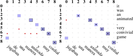
Statistical word alignment (Brown et al., 1994) is the task identifying which words are translations of each other in a bilingual sentence corpus. Figure 2 shows two examples of word alignment of a sen-tence pair. Due to the ambiguity of the word align-ment task, it is common to distinguish two kinds of alignments (Och and Ney, 2003). Sure alignments (S), represented in the figure as squares with bor-ders, for single-word translations and possible align-ments (P), represented in the figure as alignalign-ments without boxes, for translations that are either not ex-act or where several words in one language are trans-lated to several words in the other language. Possi-ble alignments can can be used either to indicated optional alignments, such as the translation of an idiom, or disagreement between annotators. In the figure red/black dots indicates correct/incorrect pre-dicted alignment points.

2.1 Baseline word alignment models

We focus on the hidden Markov model (HMM) for alignment proposed by (Vogel et al., 1996). This is a generalization of IBM models 1 and 2 (Brown et al., 1994), where the transition probabilities have a first-order Markov dependence rather than a zeroth-order dependence. The model is an HMM, where the hidden states take values from the source language words and generate target language words according to a translation table. The state transitions depend on the distance between the source language words. For

source sentencesthe probability of an alignmenta

and target sentencetcan be expressed as:

p(t,a|s) =Y j

pd(aj|aj−aj−1)pt(tj|saj), (1)

whereajis the index of the hidden state (source

lan-guage index) generating the target lanlan-guage word at

index j. As usual, a “null” word is added to the

source sentence. Figure 1 illustrates the mapping be-tween the usual HMM notation and the HMM align-ment model.

2.2 Baseline training

All word alignment models we consider are nor-mally trained using the Expectation Maximization

s1 s1 s2 s3

we know the way

sabemos el camino null

usual HMM word alignment meaning

Si (hidden) source language wordi

Oj (observed) target language wordj

aij (transition) distortion model

bij (emission) translation model

Figure 1: Illustration of an HMM for word alignment.

(EM) algorithm (Dempster et al., 1977). The EM algorithm attempts to maximize the marginal likeli-hood of the observed data (s,t pairs) by repeatedly finding a maximal lower bound on the likelihood and finding the maximal point of the lower bound. The lower bound is constructed by using posterior proba-bilities of the hidden alignments (a) and can be opti-mized in closed form from expected sufficient statis-tics computed from the posteriors. For the HMM alignment model, these posteriors can be efficiently calculated by the Forward-Backward algorithm.

3 Adding agreement constraints

Grac¸a et al. (2008) introduce an augmentation of the EM algorithm that uses constraints on posteriors to guide learning. Such constraints are useful for sev-eral reasons. As with any unsupervised induction method, there is no guarantee that the maximum likelihood parameters correspond to the intended meaning for the hidden variables, that is, more accu-rate alignments using the resulting model. Introduc-ing additional constraints into the model often re-sults in intractable decoding and search errors (e.g., IBM models 4+). The advantage of only constrain-ing the posteriors durconstrain-ing trainconstrain-ing is that the model remains simple while respecting more complex re-quirements. For example, constraints might include “one word should not translate to many words” or that translation is approximately symmetric.

distributionpθ(z|x)(wherezare the alignments). In

regular EM,pθ(z|x)is used to complete the data and

compute expected counts. Instead, we find the distri-butionqthat is as close as possible topθ(z|x)in KL

subject to constraints specified in terms of expected values of featuresf(x,z)

arg min q

KL(q(z)||pθ(z|x)) s.t. Eq[f(x,z)]≤b.

(2)

The resulting distribution q is then used in place

of pθ(z|x) to compute sufficient statistics for the

M-step. The algorithm converges to a local maxi-mum of the log of the marginal likelihood,pθ(x) = P

zpθ(z,x), penalized by the KL distance of the

posteriorspθ(z|x) from the feasible set defined by

the constraints (Grac¸a et al., 2008):

Ex[logpθ(x)− min

q:Eq[f(x,z)]≤b

KL(q(z)||pθ(z|x))],

whereExis expectation over the training data. They

suggest how this framework can be used to encour-age two word alignment models to agree during training. We elaborate on their description and pro-vide details of implementation of the projection in Equation 2.

3.1 Agreement

Most MT systems train an alignment model in each direction and then heuristically combine their pre-dictions. In contrast, Grac¸a et al. encourage the models to agree by training them concurrently. The intuition is that the errors that the two models make are different and forcing them to agree rules out errors only made by one model. This is best ex-hibited in the rare word alignments, where one-sided “garbage-collection” phenomenon often oc-curs (Moore, 2004). This idea was previously pro-posed by (Matusov et al., 2004; Liang et al., 2006) although the the objectives differ.

In particular, consider a feature that takes on value

1 whenever source wordialigns to target wordjin

the forward model and -1 in the backward model. If this feature has expected value 0 under the mixture of the two models, then the forward model and

back-ward model agree on how likely source wordiis to

align to target wordj. More formally denote the for-ward model−→p(z)and backward model←−p(z)where

−

→_{p(z) = 0for z ∈/} −→_{Z and}←−_{p(z) = 0forz ∈/} ←_Z−

(−→Zand←Z−are possible forward and backward align-ments). Define a mixturep(z) = 1₂−→p(z) + 1₂←−p(z)

forz ∈ ←Z−∪−→Z. Restating the constraints that en-force agreement in this setup:Eq[f(x,z)] =0with

fij(x,z) = 8 > <

> :

1 z∈−→Zandzij= 1 −1 z∈←Z−andzij= 1

0 otherwise

.

3.2 Implementation

EM training of hidden Markov models for word alignment is described elsewhere (Vogel et al., 1996), so we focus on the projection step:

arg min q

KL(q(z)||pθ(z|x)) s.t. Eq[f(x,z)] = 0.

(3) The optimization problem in Equation 3 can be effi-ciently solved in its dual formulation:

arg min λ

logX z

pθ(z|x) exp{λ>f(x,z)} (4)

where we have solved for the primal variablesqas:

qλ(z) =pθ(z|x) exp{λ>f(x,z)}/Z, (5)

withZa normalization constant that ensuresqsums

to one. We have only one dual variable per con-straint, and we optimize them by taking a few gra-dient steps. The partial derivative of the objective

in Equation 4 with respect to feature i is simply

Eqλ[fi(x,z)]. So we have reduced the problem to

computing expectations of our features under the

model q. It turns out that for the agreement

fea-tures, this reduces to computing expectations under the normal HMM model. To see this, we have by the definition ofqλandpθ,

qλ(z) = −

→_{p(z|x) +}←−_p(z|x)

2 exp{λ

>

f(x,z)}/Z

= −

→_{q(z) +}←−_q(z)

2 .

(To make the algorithm simpler, we have assumed

that the expectation of the feature f0(x,z) =

{1 if z ∈ −→Z; −1 if z ∈ ←Z−} is set to zero to ensure that the two models−→q ,←−q are each properly normalized.) For−→q, we have: (←−q is analogous)

−

→_p(z|x)eλ>f(x,z)

= Y

j − →_p

d(aj|aj−aj−1)−→pt(tj|saj)

Y

ij

eλijfij(x,zij)

= Y

j,i=aj − →_p

d(i|i−aj−1)−→pt(tj|si)eλijfij(x,zij)

= Y

j,i=aj − →_p

Where we have let−→p0_t(tj|si) =→−pt(tj|si)eλij, and

retained the same form for the model. The final pro-jection step is detailed in Algorithm1.

Algorithm 1AgreementProjection(−→p ,←−p)

1: λij ←0 ∀i, j 2: forT iterationsdo

3: −→p0_t(j|i)← −→pt(tj|si)eλij ∀i, j 4: ←−p0_t(i|j)← ←−pt(si|tj)e−λij ∀i, j 5: −→q ←forwardBackward(−→p0_t,−→pd) 6: ←−q ←forwardBackward(←p−0_t,←−pd)

7: λij ←λij−E−→q[ai=j] +E←−q[aj =i]∀i, j 8: end for

9: return (−→q ,←−q)

3.3 Decoding

After training, we want to extract a single alignment from the distribution over alignments allowable for the model. The standard way to do this is to find the most probable alignment, using the Viterbi al-gorithm. Another alternative is to use posterior de-coding. In posterior decoding, we compute for each

source wordiand target wordjthe posterior

prob-ability under our model that i aligns to j. If that probability is greater than some threshold, then we include the pointi−jin our final alignment. There are two main differences between posterior ing and Viterbi decoding. First, posterior decod-ing can take better advantage of model uncertainty: when several likely alignment have high probabil-ity, posteriors accumulate confidence for the edges common to many good alignments. Viterbi, by con-trast, must commit to one high-scoring alignment. Second, in posterior decoding, the probability that a

0 1 2 3 4 5 6 7 8 0 1 2 3 4 5 6 7 8

0 · · · 0 · · · it

1 · · · 1 · · · was

2 · · • · · · 2 · · • · · · an

3 · · · · • · · · · 3 • · · · • · · · · animated

4 · · · • · · · 4 · · · • · · · ,

5 · · • · · · • · · 5 · · · • · · very

6 • · · • • • · • · 6 · · · • · convivial

7 • · · · 7 • · · · game

8 · · · • 8 · · · • .

jug

abande una maneraanimaday muycordial. jugabande una maneraanimaday muycordial.

Figure 2: An example of the output of HMM trained on 100k the EPPS data. Left: Baseline training. Right: Us-ing agreement constraints.

target word aligns to none or more than one word is much more flexible: it depends on the tuned thresh-old.

4 Word alignment results

We evaluated the agreement HMM model on two corpora for which hand-aligned data are widely available: the Hansards corpus (Och and Ney, 2000) of English/French parliamentary proceedings and the Europarl corpus (Koehn, 2002) with EPPS an-notation (Lambert et al., 2005) of English/Spanish. Figure 2 shows two machine-generated alignments of a sentence pair. The black dots represent the ma-chine alignments and the shading represents the hu-man annotation (as described in the previous sec-tion), on the left using the regular HMM model and on the right using our agreement constraints. The figure illustrates a problem known as garbage collec-tion (Brown et al., 1993), where rare source words tend to align to many target words, since the prob-ability mass of the rare word translations can be hijacked to fit the sentence pair. Agreement con-straints solve this problem, because forward and backward models cannot agree on the garbage col-lection solution.

Grac¸a et al. (2008) show that alignment error rate (Och and Ney, 2003) can be improved with agree-ment constraints. Since AER is the standard metric for alignment quality, we reproduce their results us-ing all the sentences of length at most 40. For the Hansards corpus we improve from 15.35 to 7.01 for

the English→ French direction and from 14.45 to

6.80 for the reverse. For English→Spanish we

im-prove from 28.20 to 19.86 and from 27.54 to 19.18 for the reverse. These values are competitive with other state of the art systems (Liang et al., 2006).

Unfortunately, as was shown by Fraser and Marcu (2007) AER can have weak correlation with transla-tion performance as measured by BLEU score (Pa-pineni et al., 2002), when the alignments are used to train a phrase-based translation system. Conse-quently, in addition to AER, we focus on precision and recall.

65 70 75 80 85 90 95 100

1 10 100 1000 Thousands of training sentences

Agreement Baseline 65 70 75 80 85 90 95 100

1 10 100 1000 Thousands of training sentences

Agreement Baseline

Figure 3: Effect of posterior constraints on precision (left) and recall (right) learning curves for Hansards En→Fr.

10 20 30 40 50 60 70 80 90 100

1 10 100 1000

Thousands of training sentences Rare

Common Agreement

Baseline 10

20 30 40 50 60 70 80 90 100

1 10 100 1000

Thousands of training sentences Rare

Common Agreement Baseline

Figure 4: Left: Precision. Right: Recall. Learning curves for Hansards En→Fr split by rare (at most 5 occurances) and common words.

use Viterbi decoding, with larger improvements for small amounts of training data. We see a similar im-provement on the EPPS corpus.

Motivated by the garbage collection problem, we also analyze common and rare words separately. Figure 4 shows precision and recall learning curves for rare and common words. We see that agreement constraints improve precision but not recall of rare words and improve recall but not precision of com-mon words.

As described above an alternative to Viterbi de-coding is to accept all alignments that have probabil-ity above some threshold. By changing the thresh-old, we can trade off precision and recall. Figure 5 compares this tradeoff for the baseline and agree-ment model. We see that the precision/recall curve for agreement is entirely above the baseline curve, so for any recall value we can achieve higher preci-sion than the baseline for either corpus. In Figure 6 we break down the same analysis into rare and non rare words.

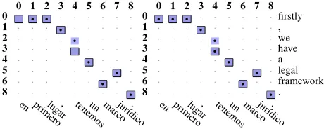
Figure 7 shows an example of the same sentence, using the same model where in one case Viterbi coding was used and in the other case Posterior de-coding tuned to minimize AER on a development set

0 0.2 0.4 0.6 0.8 1

0 0.2 0.4 0.6 0.8 1

Recall Precision Baseline Agreement 0 0.2 0.4 0.6 0.8 1

0 0.2 0.4 0.6 0.8 1

Recall

Precision Baseline Agreement

Figure 5: Precision and recall traoff for posterior de-coding with varying threshold. Left: Hansards En→Fr. Right: EPPS En→Es.

0 0.2 0.4 0.6 0.8 1

0 0.2 0.4 0.6 0.8 1

Recall Precision Baseline Agreement 0 0.2 0.4 0.6 0.8 1

0 0.2 0.4 0.6 0.8 1

Recall

Precision Baseline Agreement

Figure 6: Precision and recall trade-off for posterior on Hansards En→Fr. Left: rare words only. Right: common words only.

was used. An interesting difference is that by using posterior decoding one can have n-n alignments as shown in the picture.

A natural question is how to tune the threshold in order to improve machine translation quality. In the next section we evaluate and compare the effects of the different alignments in a phrase based machine translation system.

5 Phrase-based machine translation

In this section we attempt to investigate whether our improved alignments produce improved machine

0 1 2 3 4 5 6 7 8 0 1 2 3 4 5 6 7 8

0 • • • · · · 0 • • • · · · firstly

1 · · · • · · · 1 · · · • · · · ,

2 · · · · • · · · · 2 · · · · • · · · · we

3 · · · · • · · · · 3 · · · · • · · · · have

4 · · · • · · · 4 · · · • · · · a

5 · · · • · 5 · · · • · legal

6 · · · • · · 6 · · · • · · framework

8 · · · • 8 · · · • .

en primerolug

ar, tenemosun marcojur´ıdico. en primerolugar, tenemosun marcojur´ıdico.

translation. In particular we fix a state of the art machine translation system1and measure its perfor-mance when we vary the supplied word alignments. The baseline system uses GIZA model 4 alignments and the open source Moses phrase-based machine translation toolkit2, and performed close to the best at the competition last year.

For all experiments the experimental setup is as follows: we lowercase the corpora, and train lan-guage models from all available data. The reason-ing behind this is that even if bilreason-ingual texts might be scarce in some domain, monolingual text should

be relatively abundant. We then train the

com-peting alignment models and compute comcom-peting alignments using different decoding schemes. For each alignment model and decoding type we train Moses and use MERT optimization to tune its pa-rameters on a development set. Moses is trained us-ing the grow-diag-final-and alignment symmetriza-tion heuristic and using the default distance base distortion model. We report BLEU scores using a script available with the baseline system. The com-peting alignment models are GIZA Model 4, our im-plementation of the baseline HMM alignment and our agreement HMM. We would like to stress that the fair comparison is between the performance of the baseline HMM and the agreement HMM, since Model 4 is more complicated and can capture more structure. However, we will see that for moderate sized data the agreement HMM performs better than both its baseline and GIZA Model 4.

5.1 Corpora

In addition to the Hansards corpus and the Europarl English-Spanish corpus, we used four other corpora for the machine translation experiments. Table 1 summarizes some statistics of all corpora. The Ger-man and Finnish corpora are also from Europarl, while the Czech corpus contains news commentary. All three were used in recent ACL workshop shared tasks and are available online3. The Italian corpus consists of transcribed speech in the travel domain and was used in the 2007 workshop on spoken

lan-guage translation4. We used the development and

1_{www.statmt.org/wmt07/baseline.html} 2_{www.statmt.org/moses/}

3

http://www.statmt.org

4

http://iwslt07.itc.it/

Corpus Train Len Test Rare (%) Unk (%) En, Fr 1018 17.4 1000 0.3, 0.4 0.1, 0.2 En, Es 126 21.0 2000 0.3, 0.5 0.2, 0.3 En, Fi 717 21.7 2000 0.4, 2.5 0.2, 1.8 En, De 883 21.5 2000 0.3, 0.5 0.2, 0.3 En, Cz 57 23.0 2007 2.3, 6.6 1.3, 3.9 En, It 20 9.4 500 3.1, 6.2 1.4, 2.9

Table 1: Statistics of the corpora used in MT evaluation. The training size is measured in thousands of sentences and Len refers to average (English) sentence length. Test is the number of sentences in the test set. Rare and Unk are the percentage of tokens in the test set that are rare and unknown in the training data, for each language.

26 28 30 32 34 36

10000 100000 1e+06

Training data size (sentences) Agreement Post-pts

Model 4 Baseline Viterbi

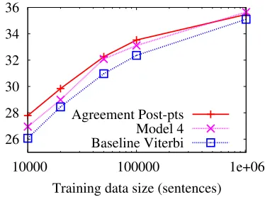
Figure 8: BLEU score as the amount of training data is increased on the Hansards corpus for the best decoding method for each alignment model.

tests sets from the workshops when available. For Italian corpus we used dev-set 1 as development and dev-set 2 as test. For Hansards we randomly chose 1000 and 500 sentences from test 1 and test 2 to be testing and development sets respectively.

Table 1 summarizes the size of the training corpus in thousands of sentences, the average length of the English sentences as well as the size of the testing corpus. We also report the percentage of tokens in the test corpus that are rare or not encountered in the training corpus.

5.2 Decoding

tune the threshold: we choose a threshold that gives the same number of aligned points as Viterbi decod-ing produces. In principle, we would like to tune the threshold by optimizing BLEU score on a devel-opment set, but that is impractical for experiments with many pairs of languages. We call this heuristic posterior-points decoding. As we shall see, it per-forms well in practice.

5.3 Training data size

The HMM alignment models have a smaller param-eter space than GIZA Model 4, and consequently we would expect that they would perform better when the amount of training data is limited. We found that this is generally the case, with the margin by which we beat model 4 slowly decreasing until a crossing point somewhere in the range of105-106sentences. We will see in section 5.3.1 that the Viterbi decoding performs best for the baseline HMM model, while posterior decoding performs best for our agreement HMM model. Figure 8 shows the BLEU score for the baseline HMM, our agreement model and GIZA Model 4 as we vary the amount of training data from

104-106sentences. For all but the largest data sizes we outperform Model 4, with a greater margin at lower training data sizes. This trend continues as we lower the amount of training data further. We see a similar trend with other corpora.

5.3.1 Small to Medium Training Sets

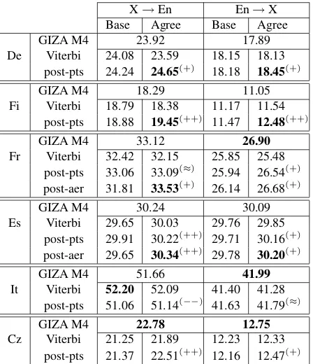
Our next set of experiments look at our perfor-mance in both directions across our 6 corpora, when we have small to moderate amounts of training data: for the language pairs with more than 100,000 sen-tences, we use only the first 100,000 sentences. Ta-ble 2 shows the performance of all systems on these datasets. In the table, post-pts and post-aer stand for posterior-points decoding and posterior decod-ing tuned for AER. With the notable exception of Czech and Italian, our system performs better than or comparable to both baselines, even though it uses a much more limited model than GIZA’s Model 4. The small corpora for which our models do not per-form as well as GIZA are the ones with a lot of rare words. We suspect that the reason for this is that we do not implement smoothing, which has been shown to be important, especially in situations with a lot of rare words.

X→En En→X

Base Agree Base Agree

GIZA M4 23.92 17.89

De Viterbi 24.08 23.59 18.15 18.13 post-pts 24.24 24.65(+)

18.18 18.45(+)

GIZA M4 18.29 11.05

Fi Viterbi 18.79 18.38 11.17 11.54 post-pts 18.88 19.45(++) _{11.47 12.48}(++)

GIZA M4 33.12 26.90

Fr Viterbi 32.42 32.15 25.85 25.48 post-pts 33.06 33.09(≈) _{25.94 26.54}(+)

post-aer 31.81 33.53(+) 26.14 26.68(+)

GIZA M4 30.24 30.09

Es Viterbi 29.65 30.03 29.76 29.85 post-pts 29.91 30.22(++) 29.71 30.16(+) post-aer 29.65 30.34(++) 29.78 30.20(+)

GIZA M4 51.66 41.99

It Viterbi 52.20 52.09 41.40 41.28 post-pts 51.06 51.14(−−) 41.63 41.79(≈)

GIZA M4 22.78 12.75

Cz Viterbi 21.25 21.89 12.23 12.33 post-pts 21.37 22.51(++) 12.16 12.47(+)

Table 2: BLEU scores for all language pairs using up to 100k sentences. Results are after MERT optimization. The marks(++)and(+)denote that agreement with poste-rior decoding is better by 1 BLEU point and 0.25 BLEU points respectively than the best baseline HMM model; analogously for(−−)_,(−)_{; while}(≈)_{denotes smaller} dif-ferences.

5.3.2 Larger Training Sets

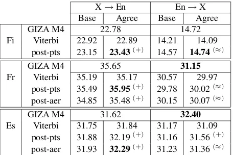
For four of the corpora we have more than 100 thousand sentences. The performance of the sys-tems on all the data is shown in Table 3. German is not included because MERT optimization did not complete in time. We see that even on over a million instances, our model sometimes performs better than GIZA model 4, and always performs better than the baseline HMM.

6 Conclusions

In this work we have evaluated agreement-constrained EM training for statistical word align-ment models. We carefully studied its effects on

word alignment recall and precision. Agreement

X→En En→X Base Agree Base Agree

GIZA M4 22.78 14.72

Fi Viterbi 22.92 22.89 14.21 14.09 post-pts 23.15 23.43(+)

14.57 14.74(≈)

GIZA M4 35.65 31.15

Fr Viterbi 35.19 35.17 30.57 29.97 post-pts 35.49 35.95(+) _{29.78 30.02}(≈)

post-aer 34.85 35.48(+) 30.15 30.07(≈)

GIZA M4 31.62 32.40

Es Viterbi 31.75 31.84 31.17 31.09 post-pts 31.88 32.19(+) 31.16 31.56(+) post-aer 31.93 32.29(+) 31.23 31.36(≈)

Table 3: BLEU scores for all language pairs using all available data. Markings as in Table 2.

can be explained by the idea that ambiguous com-mon words are different in the two languages, so the un-ambiguous choices in one direction can force the choice for the ambiguous ones in the other through agreement constraints.

To our knowledge this is the first extensive eval-uation where improvements in alignment accuracy lead to improvements in machine translation per-formance. We tested this hypothesis on six differ-ent language pairs from three differdiffer-ent domains, and found that the new alignment scheme not only per-forms better than the baseline, but also improves over a more complicated, intractable model. In or-der to get the best results, it appears that posterior decoding is required for the simplistic HMM align-ment model. The success of posterior decoding us-ing our simple threshold tunus-ing heuristic is fortu-nate since no labeled alignment data are needed: Viterbi alignments provide a reasonable estimate of aligned words needed for phrase extraction. The na-ture of the complicated relationship between word alignments, the corresponding extracted phrases and the effects on the final MT system still begs for better explanations and metrics. We have investi-gated the distribution of phrase-sizes used in transla-tion across systems and languages, following recent investigations (Ayan and Dorr, 2006), but unfortu-nately found no consistent correlation with BLEU improvement. Since the alignments we extracted were better according to all metrics we used, it should not be too surprising that they yield better translation performance, but perhaps a better trade-off can be achieved with a deeper understanding of

the link between alignments and translations.

Acknowledgments

J. V. Grac¸a was supported by a fellowship from Fundac¸˜ao para a Ciˆencia e Tecnologia (SFRH/ BD/ 27528/ 2006). K. Ganchev was partially supported by NSF ITR EIA 0205448.

References

N. F. Ayan and B. J. Dorr. 2006. Going beyond AER: An extensive analysis of word alignments and their impact on MT. InProc. ACL.

P. F. Brown, S. A. Della Pietra, V. J. Della Pietra, M. J. Goldsmith, J. Hajic, R. L. Mercer, and S. Mohanty. 1993. But dictionaries are data too. InProc. HLT. P. F. Brown, S. Della Pietra, V. J. Della Pietra, and R. L.

Mercer. 1994. The mathematics of statistical machine translation: Parameter estimation.Computational Lin-guistics, 19(2):263–311.

A. P. Dempster, N. M. Laird, and D. B. Rubin. 1977. Maximum likelihood from incomplete data via the EM algorithm. Royal Statistical Society, Ser. B, 39(1):1– 38.

A. Fraser and D. Marcu. 2007. Measuring word align-ment quality for statistical machine translation. Com-put. Linguist., 33(3):293–303.

J. Grac¸a, K. Ganchev, and B. Taskar. 2008. Expecta-tion maximizaExpecta-tion and posterior constraints. InProc. NIPS.

P. Koehn. 2002. Europarl: A multilingual corpus for evaluation of machine translation.

P. Lambert, A.De Gispert, R. Banchs, and J. B. Mari˜no. 2005. Guidelines for word alignment evaluation and

manual alignment. InLanguage Resources and

Eval-uation, Volume 39, Number 4.

P. Liang, B. Taskar, and D. Klein. 2006. Alignment by agreement. InProc. HLT-NAACL.

E. Matusov, Zens. R., and H. Ney. 2004. Symmetric word alignments for statistical machine translation. In Proc. COLING.

R. C. Moore. 2004. Improving IBM word-alignment model 1. InProc. ACL.

F. J. Och and H. Ney. 2000. Improved statistical align-ment models. InACL.

F. J. Och and H. Ney. 2003. A systematic comparison of various statistical alignment models. Comput. Lin-guist., 29(1):19–51.

K. Papineni, S. Roukos, T. Ward, and W.-J. Zhu. 2002. BLEU: A Method for Automatic Evaluation of Ma-chine Translation. InProc. ACL.