Munich Personal RePEc Archive
Pakistan-EU Commodity Trade: Is there
Evidence of J-Curve Effect?
BAHMANI-OSKOOEE, Mohsen and Iqbal, Javed and
Nosheen, Misbah and Muzammil, Muhammad
University of Wisconsin-Milwaukee, Quaid-i-Azam University,
Islamabad, Pakistan, Hazara University, Mansehra, Pakistan,
Quaid-i-Azam University, Islamabad, Pakistan
18 January 2016
1
Pakistan-EU Commodity Trade: Is there Evidence of J-Curve Effect?
Mohsen Bahmani-Oskooee1, Javed Iqbal2, Misbah Nosheen3 and Muhammad Muzammil4
Abstract
In investigating the short run and the long run impact of currency depreciation on Pakistan’s trade balance, previous studies have either relied on using bilateral trade data between Pakistan and her trade partners or between Pakistan and the rest of the world and have found not much support for successful depreciation. Suspecting that these studies may suffer from aggregation bias, in this paper we use disaggregated trade data at commodity level from 77 industries that trade between Pakistan and EU. While we find short-run significant effects in 22 industries, these effects do not last into the long run in most industries. Most of the affected industries are found to be small, as measured by their trade shares.
Keywords: J-Curve, Bound testing, commodity trade, Pakistan, EU.
JEL Classification: F31
1M. Bahmani-Oskooee, PhDCenter for Research on International Economics, University of Wisconsin-Milwaukee, Milwaukee,
WI 53201, USA, e-mail: [email protected]
2
l. INTRODUCTION
Pakistan has a history of running trade deficit. Like many other countries, it has relied
upon devaluations as well as depreciations to improve its trade balancet. The first devaluation
experienced by Pakistani rupee was in 1952. After that there are frequent instances where
Pakistani rupee has faced decline in its value. The most notable devaluation in currency value
was in 1972 and 1996. The decrease in value of rupee was expected to promote exports and
restrict imports. However, failure to see any improvement in the trade deficit could be due to
inflationary effects of nominal depreciation. For this reason we need to incorporate the nominal
exchange rate and price changes into one variable and consider changes in the real exchange rate.
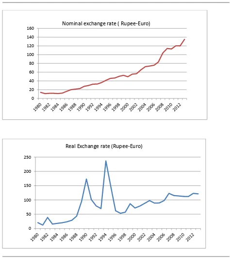
Since this paper is about Pakistan-EU trade, Figure 1 depicts the nominal and real rupee-euro
movement over our study period. As can be seen, while clearly in nominal term rupee has
depreciated, in real terms there has been periods of real depreciation and appreciation.
Figure 1 goes about here
In assessing the effects of real exchange rate changes on the trade balance, there is an
important underlying assumption that if devaluation or depreciation is to improve the trade
balance, the well-known Marshall-Lerner condition must hold. The condition basically states that
sum of import and export demand elasticities must exceed unity. Bahmani-Oskooee et al. (2013)
who provide a comprehensive review of the literature reveal that Pakistan was included in Khan
(1974) and Gylfason and Risager (1984) who used aggregate trade data and found support for the
Marshall-Lerner condition for Pakistan. However, when Akhtar and Malik (2000) disaggregated
Pakistan’s trade data by trading partners, the condition was satisfied between Pakistan and Japan
as well as U.K., but not between Pakistan and the U.S. and not between Pakistan and Germany.
3
when they used cointegration approach, they failed to find support for the Marshall-Lerner
condition in Pakistan.5
Two issues about the Marshall-Lerner condition deserve mention. First, it is a long-run
condition that must hold if currency devaluation or depreciation is to improve the trade balance.
Second, it is an indirect method of assessing the long-run effects of exchange rate changes. For
these reasons more recent studies try to establish a direct link between the trade balance and the
real exchange rate. There are a few advantages of this approach. First, this approach allows us to
account for the effects of other macroeconomic variables. Second, it allows us to distinguish the
short-run effects from the long-run effects. Indeed, the literature supports the notion that due to
adjustment lags, currency depreciation worsens the trade balance first and improves it later,
hence the J-curve effect.6 Bahmani-Oskooee (1985) who was the first to introduce a model and
the method of testing the J-curve effect was followed by Shahbaz.et al. (2009, 2011) who failed
to support the J-curve effect in Pakistan. However, Rehman an Afzal (2003) and Aftab and
Aurangzeb (2002) confirm the J- curve in Pakistan.
The above studies which found mixed results are criticized for using aggregate trade
flows of Pakistan with the rest of the world. To remedy the situation Akhtar and Malik (2000)
rely upon a model that uses bilateral trade data between Pakistan and her four major trading
partners UK, USA, Germany, and Japan. Not much support is found for the J-curve and for a
successful depreciation. The same is true of Aftab and Khan (2008) who tested the phenomenon
between Pakistan and her 12 major trading partners. Similarly, while Hameed and Kanwal
(2009) confirm positive long run relationship between the exchange rate and the trade balance,
5
Another body of the literature aims at estimating import and export demand functions separately. Examples include King (1993), Alse and Bahmani-Oskooee (1995), Charos et al. (1996),Truett and Truett (2000), Du and Zhu (2001), Love and Chandra (2005), Agbola and Damoense (2005), and Narayan and Narayan (2005).
6 See Magee (1973) for the origin and
4
they do not find support for the J-curve effect between Pakistan and her ten trade partners.
Hussian and Bashir (2012) and Bahmani-Oskooee and Cheema (2009) are other studies that also
use bilateral trade flows. The former confirms existence of J- curve between Pakistan and her
two major trade partners UK and the US, while the latter confirms the J-curve in six out of 13
Pakistan’s trading partners. Concentrating on the trade between Pakistan and one of her major
trading partners, the U.S., Bahmani-Oskooee and Cheema (2009) found no significant effect
neither in the short run nor in the long run. Failure to find significant effects was argued by
Bahmani-Oskooee et al. (2015) to be due to another aggregation bias. Once they disaggregate
Pakistan-U.S. trade flows by commodity and consider the experiences of 45 industries that trade
between the two countries, they find significant short-run effects of currency depreciation on the
trade balance of 17 industries and long-run favorable effects in 15 industries.
In this paper we add to the literature by considering the trade between Pakistan and
European Union (EU). More precisely, we investigate the short-run and long-run effects of
currency depreciation on the trade balance of 75 industries that trade between the two regions.
For this purpose, in Section II we outline the model and explain the method that is based on
Pesaran et al.’s (2001) bounds testing approach. In Section III we present the empirical results. A
summary is provided in Section IV with sources of data in an Appendix.
II. The Model and Methodology
It is now a common practice to include the level of economic activity at home, the level
of economic activity abroad and the real exchange rate as major determinants of the trade
balance. Therefore, following the literature (e.g., Bahmani-Oskooee and Xu, 2012) we adopt the
5 ) 1 ( 3 2 1 0
, t t
PAK t EU
t t
i LnY LnY LnREX
LnTB
where TBi denotes the trade balance of industry i and is defined as the ratio of Pakistan’s exports
of commodity i to EU over its import of commodity i from the EU. The measure of economic
activity in EU (Pakistan) is denoted by YEU (YPAK) and the real bilateral exchange rate by REX.
As EU grows, her imports from Pakistan (Pakistan’s exports) are expected to rise. Hence we
expect an estimate of α1 to be positive. By the same token as Pakistan’s economy grows, we
expect Pakistan to import more of commodity i. Hence, an estimate of α2 is expected to be
negative. As the Appendix shows, the real bilateral exchange rate, REX, is defined in a manner
that an increase reflects an appreciation of the euro or a depreciation of the Pakistan’s rupee.
Thus, if a real depreciation of the rupee is to have a favorable impact on the trade balance of
industry i, an estimate of α3 should be positive.
Estimate of equation (1) by any method yields only the long-run coefficient estimates.
Since the J-curve concept is a short-run phenomenon, in order to evaluate it, we need to
incorporate the short-run adjustment process into (1) by specifying it in an error-correction
format such as specification (2) below:
) 2 ( 1 4 1 3 1 2 1 , 1 0 0 0 , 1 , t t PAK t UEU t t i k t n k k t PAK k t n k k t EU k t n k k t k t i n k k t t i LnREX LnY LnY LnTB LnREX LnY LnY LnTB LnTB
Specification (2) follows Pesaran et al.’s (2001) bounds testing approach where they have
6
Cointegration among the variables then is established by applying the F test for joint significance
of lagged level variables in (2). They tabulate new critical values for this F test which accounts
for integrating properties of variables where variables could be I(0) or I(1). If variables are to be
cointegrated, the calculated F statistic should exceed the upper bound critical value that Pesaran
et al. (2001) provide. Once cointegration is established, estimates of λ2-λ4 normalized on λ1 will
yield long-run effects. The short-run effects are embodied in the estimates of coefficients
attached to first-differenced variables. The J-curve effect is confirmed when estimates of π are
negative at lower lags and positive at higher lags. We estimate error-correction model (2) for
each of the 75 industries in the next section.7
III. The Results
In this section error-correction model (2) is estimated for each of the 77 industries that
trade between Pakistan and EU using annual data over the period 1980-2013. However, as a
preliminary exercise and in order to update previous research we first estimate the model using
total trade between Pakistan and EU. Since data are annual, following the literature a maximum
of four lags are imposed on each first-differenced variable and SBC criterion is used to select
optimum number of lags or optimum model. Therefore, the reported results belonging to an
optimum model for each industry as well as for total trade. While Table 1 reports coefficient
estimates, Table 2 reports diagnostic statistics.
Tables 1 and 2 go about here
7
7
Due to volume of the estimates, we have restricted ourselves to reporting short-run
estimates for the real exchange rate only. However, long-run coefficient estimates are reported
for all three exogenous variables. From the first row in Table 1 which reports the results for total
trade model it is clear that no short-run estimate is significant. The same is true of long-run
coefficient estimates. At the 10% significance level, only EU income carries a significant
coefficient with a negative sign. This negative coefficient implies that as EU grows, it produces
more of import-substitute goods and imports less from Pakistan (Bahmani-Oskooee, 1986). As
mentioned before, these results using aggregate bilateral trade flows suffer from aggregation
bias. Clearly, there could be some industries that may react to exchange rate changes. In order to
identify these industries, we shift to estimates of error-correction model (2) for each of the 75
industries.
From the short-run estimates, we gather that at the 10% level of significance there are 21
industries in which the real exchange rate carries at least one significant coefficient. Therefore,
unlike the results using total trade flows, trade balance of 21 industries react to exchange rate
changes in the short run. However, only in industries coded 073 and 723 negative coefficients
are followed by positive ones, supporting the J-curve effect. Furthermore, while the first industry
is small measured by its trade share, the second industry is relatively large, having 2.62% of
trade share. If we rely upon Rose and Yellen (1989) and define the J-curve as short-run negative
effects combined with long run positive effects, then we can add industries 276, 540 and 667 to
the list since the real exchange rate carries significantly positive coefficient in the long run.
Clearly, the real rupee-euro rate does not play any major role in the trade between the two
regions. Nor do the level of economic activities. Pakistan’s own income carries expectedly
8
893, and 894 and EU income carries expectedly positive and significant coefficient in industries
coded 052, 247, 652, and 893.
Staying with the long-run estimates, there are only 14 industries in which at least one of
the exogenous variables carry significant coefficient. These industries are coded as 052, 073,
121, 247, 276, 540, 553, 652, 665, 681, 718, 892, 893, and 894. In order for the long-run
estimates not to be spurious, we need to establish cointegration. To this end we shift to Table 2
which reports the results of the F test along with several other diagnostics. Given its critical
value of 3.53, clearly our calculated F statistic is significant and supports cointegration in all of
these industries except in 553, 893, and 894.8 In these industries we use an alternative test which
is based on lagged error-correction term. Under this approach, long-run normalized coefficient
estimates and long-run model (1) are used to generate the error term, called usually
error-correction term denoted by ECM. Then linear combination of lagged level variables is replaced
by ECMt-1 and each model is re-estimated at the same optimum lags. A significantly negative
coefficient obtained for ECMt-1 will support cointegration or convergence toward long-run
equilibrium. However, this ECM test has new critical values that Banerjee et al. (1998, Table 1) tabulate.
Given their critical value of -3.67, cointegration is not supported in any of remaining three industries. The fact
ECMt-1 carries a significantly negative coefficient in 47 industries implies that we have estimated equilibrium
models.
Several other statistics are also reported in Table 2. To test for serial correlation in each optimum
model, we report the Lagrange Multiplier test (LM) statistic. This statistic has a χ2 distribution with
one degree of freedom. Given its critical value of 3.84 at the 5% level of significance, this
statistic is significant only in industries coded 621, 629, 666, 691, and 717. Thus, in 69 optimum
8 Note that since our sample is small, we use critical values tabulated by Narayan (2005, p. 1987). Pesaran et al.’s
9
models residuals are autocorrelation free. Table 2 also reports Ramsey’s RESET statistic which
is used to identify misspecified models. It also has χ2 with one degree of freedom. This statistic is
significant only in 11 models coded 062, 276, 540, 629, 666, 671, 681, 831, 890, 893, and 897.
This, only 11 optimum models are misspecified. In order to establish stability of short-run and
long-run coefficient estimates, we follow Brown et al. (1975) and apply their CUSUM and
CUSUMSQ tests to the residuals of each optimum model. We have indicated stable coefficients
by “S” and unstable ones by “US”. Clearly, almost all estimates are stable.9 Lastly, we have
reported the size of adjusted R2 so that we can judge the goodness of fit.
IV. Summary and Conclusion
A steady depreciation of Pakistani rupee and its impact on Pakistan’s trade balance has been the focus of many previous studies. They have either relied upon estimating the indirect
approach of Marshall-Lerner condition or direct approach of relating the trade balance to its
determinants such as income levels and the real exchange rate. No matter which approach was
used, not much support was found for favorable effects of depreciation on Pakistan’s trade balance. These studies used either aggregate trade flows of Pakistan with the rest of the world or
bilateral trade flows between Pakistan and it major trading partners.
Suspecting that previous studies may suffer from aggregation bias, our intention in this
paper is to consider the impact of currency depreciation on the trade balance between Pakistan
and European Union (EU). We test for the short-run effects, hence the J-curve and the long-run
effects using Pesaran et al.’s (2001) bounds testing approach using aggregate trade flows
between the two regions first. Since no short-run effects and no long-run effects are discovered,
we disaggregate the trade flows by commodity and estimate a trade balance model for each of
the 77 industries that trade between the two regions. We find significant short-run effects in 21
industries. However, the short-run effects lasted into long-run favorable effects only in two
industries.
9
10
APPENDIX
Data Definition and Sources
Empirical analysis is based on annual data over the period 1980-2013. Data come from the
following sources:
a. World Bank
b. International Financial Statistics
Variable Definitions
TBi= measure of trade balance for industry i defined as the ratio of Pakistan exports of
commodity i to EU over its import of commodity i from EU. Industry level data come from
source a.
YPAk = Pakistan’s income measured by its real GDP. Data come from source b. YEU = EU income measured by its real GDP. Data come from source b.
REX= Real bilateral exchange rate between Euro and Pakistani Rupee. It is defined as
(CPIEU * NEX / CPIPAK ) where NEX is the nominal bilateral exchange rate defined as number
rupees per euro and CPI is price level. Thus, an increase in REX is a reflection of real
11
References
Aftab Z. and Khan S. (2008). Bilateral j-curve between Paksitan and her trading partners, PIDE working paper No 2008:45.
Aftab Z. and Aurangzeb (2002). The long run and short run impact of exchange rate devaluation on Pakistan’s trade performance, The Pakistan Development Review, 4(3); 277-286.
Agbola, F. W. and M. Y. Damoense, 2005. “Time-Series estimation of import demand functions for India”, Journal of Economic Studies, 32: 146-157.
Akhtar, S. and Malik, F. (2000). Pakistan Trade Performance Vis-a- vis its Major Trading Partners. The Pakistan Development Review, 39(1), 37-50.
Alse, J. and M. Bahmani-Oskooee, 1995. Do devaluations improve or worsen the terms of trade? Journal of Economic Studies, 22: 16-25.
Bahmani-Oskooee, M. 1985). Devaluation and j-curve: Some Evidence from LDCs. The Review of Economic and Statistics, 500–504.
Bahmani-Oskooee, M. 1986, Determinants of international trade flows: The case of developing countries. Journal of Development Economics, 20: 107-123.
Bahmani-Oskooee, M. and O. Kara, 2005. Income and price elasticities of trade: Some new estimates. International Trade Journal, 19: 165-178.
Bahmani-Oskooee, M. and S.W. Hegerty, 2007. Exchange rate volatility and trade flows: A review article. Journal of Economic Studies, 34: 211-255
Bahmani-Oskooee, M. and A. Gelan, 2009. How stable is the demand for money in African countries.
Journal of Economic Studies, 36: 216-235
Bahmani-Oskooee, M., Cheema, J., (2009). Short-run and long-run effects of currency depreciation on the bilateral trade balance between Pakistan and her major trading partners.
Journal of Economic Development, 34(1), 19-46.
Bahmani-Oskooee, M. and S. Hegerty, (2010),“The J- and S-Curves: A Survey of the Recent Literature”, Journal of Economic Studies, Vol. 37, pp. 580-596.
Bahmani-Oskooee and Xu (2012), “Is there Evidence of the J-Curve in Commodity Trade between the U.S. and Hong Kong?”, The Manchester School, Vol. 80, pp. 295-320.
Bahmani-Oskooee, M., C. Economidou, and G. G. Goswami., 2005. How sensitive are Britain’s inpayments and outpayments to the value of the British pound? Journal of Economic Studies, 32: 455-467.
12
Equation Framework,” Journal of Time Series Analysis 19, 267–85.
Brown, R. L., J. Durbin, and J. M. Evans (1975), "Techniques for Testing the Constancy of Regression Relations Over Time", Journal of the Royal Statistical Society, Series B, Vol. 37, (1975), pp. 149-163
Charos, E. N., E. O. Simos, and A. R. Thompson, 1996. Exports and industrial growth: A new framework and evidence. Journal of Economic Studies, 23: 18-31.
Chen, S.-W. and T.-C. Chen, 2012. Untangling the non-linear causal nexus between exchange rates and stock prices: new evidence from the OECD countries. Journal of Economic Studies, 39: 231-259.
Dell’Anno, R. and Halicioglu, F., 2010. An ARDL model of recorded and unrecorded economies in Turkey. Journal of Economic Studies, 37: 627-646.
De Vita, G. and K. S. Kyaw, 2008. Determinants of capital flows to developing countries: A structural VAR analysis. Journal of Economic Studies, 35: 304-322.
Du, H. and Z. Zhu, 2001. The effect of exchange-rate risk on exports: Some additional empirical evidence. Journal of Economic Studies, 28: 106-121.
Gylfason, T. and O. Risager, 1984. Does devaluation improve the current account?, European Economic Review, 25: 37-64.
Hajilee, Massomeh, and Omar M. Al-Nasser, (2014), “Exchange Rate Volatility and Stock Market Development in Emerging Economies”, Journal of Post Keynesian Economics, Vol. 37, pp. 163-180.
Halicioglu, F., 2007. The J-curve dynamics of Turkish bilateral trade: A cointegration approach. Journal of Economic Studies, 34: 103-119.
Halicioglu, F. (2013) “Dynamics of Obesity in Finland”, Journal of Economic Studies, Vol.40, pp. 644-657.
Hameed, A. and S. Kanwal. (2009). Existence of a J-Curve-The Case of Pakistan”. Journal of Economic Cooperation and Development. 30 (2) :75-98.
Hussain M. and Bashir, U. (2012). Dynamics of Trade Balance and the J-Curve Phenomenon: Evidence from Pakistan. Journal of Commerce, Vol. 5 (Issue 2), pp. 16-31.
Khan, Mohsin S. (1974), “Import and Export Demand in Developing Countries”, IMF Staff Papers, Vol. 21, pp. 678-693.
King, A., 1993. The functional form of import demand: The Case of UK motor vehicle imports, 1980-90.
Journal of Economic Studies, 20: 36-50.
Love, J. and R. Chandra, 2005. Testing export-led growth in South Asia. Journal of Economic Studies,
13
Magee, S.P. (1973). Currency Contracts, Pass Through and Devaluation, Brooking Papers on Economic Activity, 1, 303-325.
Mohammadi, H., M. Cak, and D. Cak, 2008. Wagner’s hypothesis: New evidence from Turkey using the bounds testing approach., Journal of Economic Studies, 35: 94-106.
Narayan, P.K., 2005. The saving and investment nexus for China: Evidence from cointegration tests.
Applied Economics, 37: 1979-1990.
Narayan, S. and P. K. Narayan, 2005. An empirical analysis of Fiji’s import demand function. Journal of Economic Studies, 32: 158-168.
Narayan, P.K., S. Narayan, B.C. Prasad, and A. Prasad, 2007. Export-led growth hypothesis: Evidence from Papua New Guinea and Fiji. Journal of Economic Studies, 34: 341-351.
Payne, J. E., 2008. Inflation and inflation uncertainty: Evidence from the Caribbean region. Journal of Economic Studies, 35: 501-511.
Pesaran, M.H., Y. Shin and R.J. Smith,( 2001). Bounds testing approaches to the analysis of level relationships. J. Applied Econometrics, 16: 289-326.
Rehman, H. and Afzal, M. (2003). J-curve Phenomenon: An Evidence from Pakistan. Pakistan Economic and Social Review, 41(1), 45-57.
Rose, A.K., and Yellen, J.L. 1989. Is There a J-Curve? Journal of Monetary Economics 24(1), 53-68.
Shahbaz, M., (2009). On nominal and real devaluations relation: an econometric evidence for Pakistan, International Journal of Applied Econometrics and Quantitative Studies, 9, pp, 86-108.
Shahbaz, M., Awan, R. U., Ahmad, K., (2011). The exchange value of the Pakistan rupee & Pakistan trade balance: An ARDL bounds testing approach. The Journal of Developing Areas, 44, 69-93.
Tang, T.C., 2007. Money demand function for Southeast Asian countries: An empirical view from expenditure components. Journal of Economic Studies, 34: 476-496.
Tayebi, S. K., and M. Yazdani, 2014. Financial crisis, oil shock and trade in Asia. Journal of Economic Studies, 41: 601-614.
Truett, L. J. and D. B. Truett, 2000. The demand for imports and economic reform in Spain. Journal of Economic Studies, 27: 182-199.
Wong, K. N. and T. C. Tang, 2008. The effects of exchange rate variability on Malaysia’s disaggregated electrical exports. Journal of Economic Studies, 35: 154-169.
14
Figure 1: Plot of Nominal and Real Exchange Rate
Note: The exchange rate is defined as number of rupees per euro.
0 20 40 60 80 100 120 140
160 Nominal exchange rate ( Rupee-Euro)
0 50 100 150 200 250
16
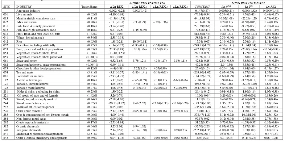
Table 1: Short-Run and Long-Run Coefficient Estimates
SHORT RUN ESTIMATES LONG RUN ESTIMATES
SITC INDUSTRY Trade Shares ∆ Ln REXt ∆ Ln REXt-1 ∆ Ln REXt-2 ∆ Ln REXt-3 CONSTANT Ln YPAK Ln YEU Ln REX
Aggregate industry -0.002(-0.22) -0.002(0.42) 0.147(0.87) 0.005(0.21) -0.009(1.82) 0.0009(0.46)
001 Live animals (0.02)% -4.10(-0.68) -76.14(-0.34) -2.59(-0.51) 4.76(0.43) -0.48(-0.17)
013 Meat in airtight containers n.e.s (0.11)% -11.36(-1.73) 441.85(1.03) 10.02(1.08) -22.29(-1.20 -4.78(-0.82)
022 Milk and cream (0.20)% -1.71(-0.31) 2.33(0.29) -7.93(-1.36) -7.11(-0.03) 0.79(0.17) -0.50(-0.05) 0.49(0.19)
031 Fish, fresh & simply preserved (0.18)% -3.54(-0.40) 221.69(0.63) 2.69(0.34) -9.27(-0.53) -2.25(-0.54)
032 Fish, in airtight containers, n.e.s (0.18)% 0.31(0.25) -1.45(-0.39) 79.81(0.43) -1.78(-0.07) -0.62(-0.07) -3.53(-1.49)
033 Fruit, fresh, and nuts excl. Oil nuts (1.42)% 0.27(0.03) 518.66(1.46) 9.80(1.23) -24.94(1.43) -3.06(-0.68)
041 Wheat including spelt (0.34)% -2.38(-0.18) -58.92(-0.11) -5.56(-0.40) 7.10(0.26) -3.18(-0.46)
042 Rice (0.05)% 1.88(0.21) -10.09(0.81) -17.54(-0.05) -2.16(-0.28) 2.56(0.16) -1.11(-0.26)
052 Dried fruit including artificially (0.72)% -1.14(-0.27) -1.83(-0.41) -3.51(-0.88) -248.75(-1.72) -4.33(-1.41) 11.84(1.74) 0.28(0.14)
053 Fruit, preserved and fruit preparations (0.03)% 22.83(0.88) 10.11(1.04) 11.56(0.51) 677.18(0.73) 2.71(0.15) -23.06(1.54) -10.64(-0.81)
054 Vegetables, roots & tubers, fresh (1.08)% -13.40(-3.55) -99.41(-0.71) 1.34(0.43) 1.72(0.25) 2.86(1.62)
055 Vegetables, roots & tubers preserved (0.001)% 0.03(0.01) -24.28(-0.31 -0.07(-0.04) 0.68(0.18) 1.15(1.16)
061 Sugar and honey (0.02)% 6.52(1.63) 5.78(1.21) 4.34(1.17) 3.58(1.11) -42.82(-0.28) -2.80(-0.83) 3.85(0.52) -0.55(-0.29)
062 Sugar confectionery, sugar preparations. (0.004)% -0.49(-0.11) -47.28(-0.28) -2.3(-0.56) 3.55(0.41) -0.23(-0.11)
073 Chocolate & other food preparations. (0.12)% -4.4(-0.88) 17.22(3.13) 4.55(0.99) 25.40(0.15) -6.20(-1.64) 4.84(0.60) -3.13(-1.27)
074 Tea and mate (5.81)% -3.11(-0.57) -3.83(-1.41) -0.19(-0.01) -203.80(-1.02) -2.67(-0.59) 8.77(0.89) 1.57(0.64)
081 Feed stuff for animals (0.25)% -7.93(-1.21) -184.07(-0.74) -1.60(-0.29) 7.14(0.58) 1.90(0.64)
112 Alcoholic beverages (0.18)% 5.17(0.42) -7.65(-0.59) 2.11(0.17) -6.60(-0.66) -3.84(-0.01) 3.99(0.44) -3.57(-0.18) 2.32(0.36)
121 Tobacco, unmanufactured (0.34)% 4.65(0.56) -14.49(-1.54) 3.12(0.44) 469.87(1.70) 9.02(1.46) -22.38(1.70) -4.88(-1.21)
122 Tobacco manufactured (0.07)% 4.96(0.45) 0.11(0.01) 0.20(0.02) 5.20(0.59) 284.42(0.74) 5.64(0.70) -13.74(0.77) -2.60(-0.46)
211 Hides & skins, excluding fur skins (0.23)% 1.30(0.22) -26.41(-0.12) -0.91(-0.18) 1.80(0.16) -1.07(-0.38)
221 Oil seeds, oil nuts and oil kernels (1.42)% 5.26(0.79) -10.00(-0.04) 0.21(0.03) 0.03(0.001) 0.83(0.26)
243 Wood, shaped or simply worked (0.24)% -2.58(-1.01) 11.21(0.12) 0.60(0.29) -0.96(-0.21) 0.54(0.46)
244 Wood manufactures, n.e.s (0.02)% -20.11(-3.72) 9.61(2.57) -17.68(-2.33) -10.68(-3.20) -193.58(-0.86) 1.35(1.22) 4.67(1.10) 3.82(1.04)
247 Works of art, collectors pieces (0.03)% 0.65(0.06) -235.63(1.70) -4.67(-2.03) 11.60(3.48) 0.87(0.04)
276 Other crude minerals (0.05)% -2.12(-0.62) -0.65(-0.06) 1.38(0.16) -0.98(-0.12) 18.04(1.42) 4.65(1.22) -4.90(-1.23) 2.69(1.88)
283 Ores & concentrates of non-ferrous metals (0.06)% -4.00(-0.46) -378.47(-1.20) -5.11(-0.72) 16.02(1.04) 5.25(1.32)
284 Non-ferrous metal scrap (0.06)% 0.09(0.02) -97.57(-0.62) -0.12(-0.04) 2.92(0.38) 2.75(1.38)
292 Crude vegetable materials (0.17)% -2.73(-1.84) 31.22(0.55) 0.72(0.56) -1.59(-0.57) -0.32(-0.46)
512 Organic chemicals (0.04)% 5.25(1.01) 6.94(1.02) -32.70(-2.20) -1.97(-0.32) 2.87(0.39) -0.84(-0.52)
540 Inorganic chemicals (0.03)% 2.14(0.58) -2.14(-1.60) 3.25(0.64) 0.94(0.23) -232.18(-1.35) -1.02(-0.58) 8.33(1.09) 5.83(2.07)
541 Medicinal & pharmaceutical products (2.51)% -0.13(-0.08) 0.29(0.001) -0.54(-0.41) 0.50(0.17) -0.37(-0.50
17
553 Perfumery, cosmetics, dentifrices, etc. (0.07)% 4.73(2.28) 2.29(0.79) 4.18(1.90) -7.40(-0.11) -3.43(-2.03) 3.33(1.01) -1.32(-1.17)
554 Soaps, cleansing & polishing preparations (3.39)% 4.41(-0.03) -38.24(-0.20) -1.49(-0.34) 2.64(0.28) -0.76(-0.31)
621 Materials of rubber (0.19)% -6.13(-0.66) -203.49(-0.59) -3.59(0.57) 9.56(0.57) 1.28(0.29)
629 Articles of rubber, n.e.s. (0.22)% -13.11(-3.48) -3.37(-0.82) -4.31(-1.39) -61.35(-0.49) 0.68(0.25) 1.39(0.23) 0.40(0.22)
631 Veneers, plywood boards & other wood (0.001)% -6.32(-1.45) -54.31(-0.33) 0.14(0.04) 1.51(0.19) 1.07(0.51)
641 Paper and paperboard (1.06)% 5.04(0.74) 151.60(0.69) 1.39(0.29) -5.84(-0.56) -2.15(-0.69)
651 Textile yarn and thread (0.15)% -3.39(-2.76) 0.68(0.05) 2.83(1.55) -0.56(0.05) 10.83(0.21) 0.65(0.55) -0.93(-0.36) 0.18(0.27)
652 Cotton fabrics, woven (0.14)% -1.62(-0.36) 4.37(1.15) -251.64(-1.70) -6.19(-1.90) 13.54(1.89) 0.001(0.001)
655 Special transactions not classified according to kind
(0.23)% 14.94(3.83) 3.98(0.19) 2.84(0.49) 0.58(0.23) 304.74(0.19) 0.36(0.01) -8.56(-1.09) -11.96(-1.43)
655 Special textile fabrics and related (0.02)% -2.63(-0.58) 74.28(0.44) 2.56(0.67) -4.69(-0.56) 0.54(0.25)
656 Made up articles, wholly or chiefly (1.13)% -15.36(-3.73) 7.59(1.72) -7.19(-2.04) -50.83(-0.37) 0.87(0.29) 0.73(0.11) 1.40(0.70)
661 Lime, cement & fabricated building materials (0.08)% 8.65(2.06) 243.49(1.65) 3.75(1.14) -10.71(1.48) -3.17(-1.70)
662 Clay and refractory construction material (0.33)% 3.29(0.45) -7.00(-0.94) -1.65(-0.28) 21.78(0.09) 3.36(0.65) -3.73(-0.33) 1.26(0.36)
664 Glass (0.20)% -1.13(-0.19) -141.45(-0.64) -2.81(-0.57) 6.92(0.64) 0.85(0.31)
665 Glassware (1.64)% 3.33(0.58) -8.13(-1.60) 3.25(0.63) 0.93(0.23) -227.18(-1.35) -2.02(-0.58) 8.33(1.09) 5.83(2.07)
666 Pottery (0.21)% -72.13(-1.03) -52.02(-2.09) 21.07(1.45) 1.19(0.22) 2.85(0.69)
671 Pig iron, spiegeleisen, sponge iron (0.01)% -9.63(-0.87) -2.34(0.59) 4.10(1.21) -0.48(0.21) -112.36(-0.51) -0.36(-0.01) 3.65(1.01) 2.39(0.81)
676 Essential oils, perfume and flavor (0.32)% 0.28(0.22) -3.78(-0.52) -0.14(-0.02) 0.23(0.41) 0.05(0.32)
681 Silver and platinum group metals (0.70)% 2.75(0.48) 53.53(0.19) 0.95(0.15) -2.52(2.11) -0.3(0.45)
682 Copper (0.13)% -1.34(0.01) 2.81(0.73) 31.72(-1.43) 1.49(-1.45) -2.23(1.53) -0.47 (0.11)
692 Metal containers for storage and transport (2.15)% 9.95(0.84) -10.15(0.84) -5.52(-0.41) -163.79(-0.55) 1.27(0.15) 3.62(0.19) 4.90(0.85)
693 Wire products (0.03)% -10.83(-1.43) -143.83(-0.55) -2.36(-0.39) 6.40(0.49) 2.17(0.68)
696 Cutlery (0.01)% 5.34(1.88) -1.39(-0.50) 38.98(0.42) -1.04(-0.50) -0.25(-0.06) -1.08(-0.85)
711 Power generating machinery (0.21)% 7.81(0.88) -1.38(-0.19) 31.41(0.11) 1.65(0.26) -2.46(-0.18) 0.26(0.07)
712 Agricultural machinery and implement (0.32)% -4.23(-0.50) 221.34(0.76) 5.57(0.87) -11.54(0.81) -2.97(-0.84)
714 Office machinery (0.13)% 0.17(1.31) 0.002(0.02) 0.101(0.82) 1.46(0.35) -0.03(-0.22) -0.01(-0.33) -0.05(-0.73)
717 Textile and leather machinery (0.04)% -0.01(0.21) 1.25(0.94) -8.74(-1.98) -31.92(0.40) 0.98(0.35) -2.39(-0.39) -0.53(-0.32)
676 Essential oils, perfume and flavor (0.32)% 0.28(0.22) -3.78(-0.52) -0.14(-0.02) 0.23(0.41) 0.05(0.32)
718 Machines for special industries (0.02)% 25.71(4.23) 9.27(1.29) -3.76(-0.62) 3.36(0.64) -200.3 (-0.99) -9.42(-2.18) 14.30(1.53) 1.60(0.51)
719 Machinery and appliances non electrical (0.95)% -0.02(-0.65) 0.04(1.55) 0.01(0.36) -0.01(0.55) -0.62(-0.73 -0.02(-1.08) 0.04(0.91) 0.01(0.39)
723 Equipment for distributing electric (2.62)% -17.09(-2.04) 15.78(1.85) 3.83(0.56) 110.71(0.41) -0.21(-0.04) -3.31(-0.26) -1.17(-0.30)
724 Telecommunications apparatus (2.22)% -5.16(-0.36) -139.84(-0.10) -2.84(-0.30) 6.97(0.21) 0.23(-0.40)
812 Sanitary, plumbing, heating & light (0.01)% -2.40(-0.39) 0.03(0.22) -1.26(-0.51) -6.51(-1.51) -0.17(-0.01) 0.37(0.11) -0.09(-0.01)
821 Furniture (0.03)% 0.78(0.35) -3.89(-0.87) -0.99(-0.35) 1.04(0.51) -0.48(-0.11)
831 Travel goods, handbags and similar articles (0.27)% -24.03(-3.69) -3.51(-0.27) -105.71(-0.60) 2.53(0.23) 0.83(0.27) 3.50(1.33)
18
851 Footwear (0.05)% 4.88(1.13) 5.01(1.08) -4.50(-1.28) -128.37(-0.91) -3.26(-1.07) 6.69(1.00) 1.91(0.94)
890 Articles of artificial matter (0.01)% 0.23(-1.89) -47.35(-0.91) -0.69(-0.84) 2.13 (0.91) 0.20(0.66)
892 Printed materials I (0.01)% 5.27(2.18) -47.60(-0.53) -3.73(-1.85) 4.93(1.12) -1.45(-1.27)
893 Articles of artificial plastic mate (0.03)% -5.90(0.43) -0.17(-0.31) `-103.7(-2.72) -2.12(-1.87) 5.07(2.63) 0.94(0.75)
894 Perambulators ,toys, games and sporting goods (0.03)% 4.70(2.45) 1.47(0.63) 3.9(2.44) -12.98(-0.20) -3.06(-2.15) 3.16(1.04) -1.04(-1.14)
897 Jewellery and gold/silver smiths wares (0.02)% -2.68(-0.51) -1.42(-0.31) -0.09(-0.11) 0.22(0.31) -0.69(0.51)
899 Manufactured articles, n.e.s (0.21)% -1.83(-1.45) 2.50(1.85) 0.36(0.25) -1.54(0.22) 23.85(0.54) 0.33(0.03) -0.76(-0.35) -0.42(-0.60)
Notes: a. Number inside the parenthesis next to each coefficient is the t-ratio.
b. Trade shares of each industry is calculated as sum of exports and imports by that industry as a per cent of sum of total exports and imports The totals includes even industries for which no data were available. These shares are only for 2013.
19
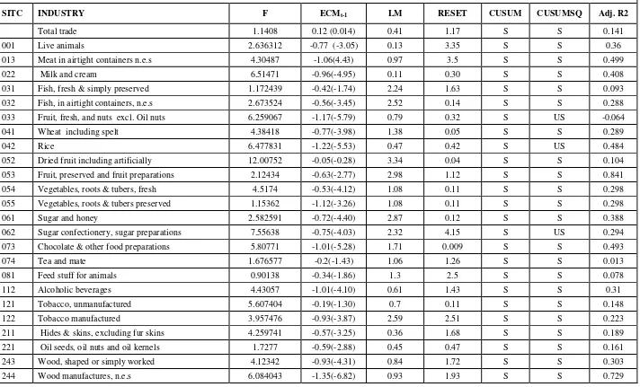
Table 2: Diagnostic Statistics
SITC INDUSTRY F ECMt-1 LM RESET CUSUM CUSUMSQ Adj. R2
Total trade 1.1408 0.12 (0.014) 0.41 1.17 S S 0.141
001 Live animals 2.636312 -0.77 (-3.05) 0.13 3.35 S S 0.36
013 Meat in airtight containers n.e.s 4.30487 -1.06(4.43) 0.97 3.5 S S 0.499
022 Milk and cream 6.51471 -0.96(-4.95) 0.11 0.30 S S 0.408
031 Fish, fresh & simply preserved 1.172439 -0.42(-1.74) 2.24 1.63 S S 0.093
032 Fish, in airtight containers, n.e.s 2.673524 -0.56(-3.45) 2.52 0.14 S S 0.288
033 Fruit, fresh, and nuts excl. Oil nuts 6.259067 -1.17(-5.79) 0.79 0.32 S US -0.064
041 Wheat including spelt 4.38418 -0.77(-3.98) 1.38 0.05 S S 0.289
042 Rice 6.477831 -1.22(-5.53) 0.47 0.42 S US 0.484
052 Dried fruit including artificially 12.00752 -0.05(-0.28) 3.34 0.04 S S 0.104
053 Fruit, preserved and fruit preparations 2.12434 -0.63(-2.77) 2.98 1.12 S S 0.841
054 Vegetables, roots & tubers, fresh 4.5174 -0.53(-4.12) 1.08 0.11 S S 0.298
055 Vegetables, roots & tubers preserved 1.15362 -1.12(-3.26) 1.08 0.11 S S 0.298
061 Sugar and honey 2.582591 -0.72(-4.40) 2.87 0.12 S S 0.388
062 Sugar confectionery, sugar preparations 7.55638 -0.75(-4.03) 2.32 4.15 S US 0.294
073 Chocolate & other food preparations 5.80771 -1.01(-5.28) 1.71 0.009 S S 0.493
074 Tea and mate 1.676577 -0.2(-1.43) 1.06 1.26 S S 0.013
081 Feed stuff for animals 0.90138 -0.34(-1.86) 1.3 2.5 S S 0.078
112 Alcoholic beverages 4.43057 -1.01(-4.10) 0.61 1.43 S S 0.31
121 Tobacco, unmanufactured 5.607404 -0.19(-1.30) 0.7 0.11 S S 0.148
122 Tobacco manufactured 3.957476 -0.93(-3.87) 2.59 2.51 S S 0.223
211 Hides & skins, excluding fur skins 4.259741 -0.57(-3.25) 0.36 1.68 S S 0.189
221 Oil seeds, oil nuts and oil kernels 1.7277 -0.59(-2.88) 0.45 0.47 S S 0.161
243 Wood, shaped or simply worked 4.12342 -0.93(-4.31) 0.84 1.72 S S 0.303
20
247 Works of art, collectors pieces 3.497327 -0.62(1.92) 2.37 12.59 S S 0.378
276 Other crude minerals 8.71301 0.29(2.66) 0.27 4.044719 S US 0.68
283 Ores & concentrates of non-ferrous metals 1.17582 -0.26(-0.47) 0.28 2.76 S S 0.329
284 Non-ferrous metal scrap 2.33423 -0.53(3.31) 1.2 0.41 S US 0.336
292 Crude vegetable materials 3.108699 -0.53(-2.67) 0.05 0.254375 US S 0.078
512 Organic chemicals 4.35933 -0.96(-5.50) 0.12 0.02 S S 0.431
540 Inorganic chemicals 3.497327 -0.62(-4.47) 2.37 12.59 S S 0.378
541 Medicinal & pharmaceutical products 1.45872 -0.77(-3.90) 0.45 2.488 S S 0.015
542 Other electrical machinery and apparatus 2.184792 -0.61(-2.16) 0.02 0.13 S US 0.145
553 Perfumery, cosmetics, dentifrices, etc. 2.70664 -0.95(-3.46) 0.7 0.7 S S 0.353
554 Soaps, cleansing & polishing preparations 1.99622 -0.72(-3.71) 1.54 0.53 S S 0.258
621 Materials of rubber 5.661642 -0.01(-0.02) 5.54 2.59 S S -0.162
629 Articles of rubber, n.e.s. 4.67312 -0.84(-4.74) 8.71 15.52 S S 0.161
631 Veneers, plywood boards & other wood 0.91253 -1.28(-7.00) 0.89 0.78 S S 0.719
641 Paper and paperboard 7.13609 -0.99(-4.47) 0.16 0.505 S US 0.349
651 Textile yarn and thread 4.326284 -0.75(-4.15) 1.23 0.017201 S S 0.375
652 Cotton fabrics, woven 3.544737 -0.09(-0.57) 2.52 0.14 S S 0.051
655 Special transactions not classified according to
kind 2.19829 -0.88(-3.90) 0.86 1.41 S S 0.456
655 Special textile fabrics and related 5.664 -1.3(-5.84) 0.36 0.27 S S 0.512
656 Made up articles, wholly or chiefly 7.083378 -0.93(-4.88) 1.23 1.323326 S US 0.625
661 Lime, cement & fabricated building materials 7.4738 -0.80(-5.61) 3.09 0.07 S S 0.52
662 Clay and refractory construction material 5.36779 -0.91(-4.20) 1.11 2.923008 S S 0.294
664 Glass 5.417447 -0.87(-4.38) 1.26 0.18 S S 0.335
665 Glassware 5.44938 -0.6(-2.66) 0.26 0.000911 S S 0.261
666 Pottery 5.8115 -1.57(-7.96) 3.95 5.53 S S 0.759
671 Pig iron, spiegeleisen, sponge iron 4.815270 -0.86(-3.76) 0.71 13.74 S S 0.609
21
681 Silver and platinum group metals 10.45241 -0.03(-0.39) 0.11 3.97 S S -0.346
682 Copper 1.544737 -0.21(-1.32) 1.31 1.05 S S 0.125
692 Metal containers for storage and transport 6.728833 -1.36(-6.46) 2.16 0.28 S S 0.575
693 Wire products 2.328685 -0.84(-3.67) 0.35 0.493456 S S 0.314
696 Cutlery 2.34815 -0.53(3.07) 0.04 3.44 S S 0.308
711 Power generating machinery 8.84263 -0.91(-4.38) 0.731403 1.24 US S 0.303
712 Agricultural machinery and implement 2.59221 -0.75(-4.66) 0.11 0.04 S S 0.513
714 Office machinery 3.209342 -1.17(-5.03) 0.3 2.480104 S US 0.423
717 Textile and leather machinery 16.82966 -1.28(-6.33) 6.27 0.18 S S 0.586
718 Machines for special industries 8.5287 -1.39(-6.70) 2.85 1.3 S S 0.729
719 Machinery and appliances non electrical 13.41448 -1.44(-6.78) 0.4 0.45 S S 0.621
723 Equipment for distributing electricity 8.3424 -0.75(-3.61) 1.01 11.4 S S -0.073
724 Telecommunications apparatus 7.4078 -1.00(-5.43) 0.06 0.13 S S 0.473
812 Sanitary, plumbing, heating & light 3.00975 -0.74(-3.81) 2.49 0.496034 S S 0.239
821 Furniture 5.82728 -0.65(3.45) 0.68 2.51 S S 0.19
831 Travel goods, handbags and similar articles 8.19318 -1.02(-5.02) 0.24 4.54 S US 0.475
841 Clothing except fur clothing 2.476322 -0.86(-3.96) 0.59 1.442178 S S 0.222
851 Foot ware 3.01861 -0.83(-4.22) 2.22 3.64 S S 0.429
890 Articles of artificial matter 2.55067 -0.72(-2.69) 2.32 4.29 S US 0.321
892 Printed material 5.811875 -0.65(-3.70) 1.88 0.3 S S -0.196
893 Articles of artificial plastic material 2.550673 -0.72(0.004) 2.32 4.29 S US 0.321
894 Perambulators ,toys, games and sporting goods 1.823073 -0.86(4.55) 0.08 0.225022 S S 0.577
897 Jewellery and gold/silver smiths wares 5.105120 -0.79(4.01) 2.65 3.93 S S 0.323
899 Manufactured articles, n.e.s 2.03556 -0.67(-5.24) 0.4 0.008477 S S 0.389
a. LM: Lagrange multiplier test of residual serial correlation. b. RESET: Ramsey’s test for function form.
c. CUSUM: Cumulative Sum of Recursive Residuals
d. CUSUMSQ: Cumulative Sum of Squares of Recursive Residuals