Munich Personal RePEc Archive
Monetary Policy, Fiscal Policy, and
Secular Stagnation at the Zero Lower
Bound. A View on the Eurozone
Kleczka, Mitja
Leibniz University Hannover
30 September 2015
Online at
https://mpra.ub.uni-muenchen.de/67228/
Monetary Policy, Fiscal Policy, and
Secular Stagnation at the Zero Lower Bound.
A View on the Eurozone
Mitja Kleczka October 2015 Email: kleczka@mail.de Phone: +49 177 7616454
Abstract: This paper delivers a contemporary estimate of the Eurozone’s natural real rate of interest. While it is found that the natural real rate has declined substantially between 1997 and 2015, it has not become negative. Thus, even in the presence of low inflation and nominal interest rates at the zero lower bound, the Eurozone does not face an acute threat of secular stagnation as defined by Lawrence Summers. Similarly, it is deemed unlikely that a number of ‘headwinds’ or a demise of technological growth will lead to a secular decline of the
Eurozone’s economic growth. At the same time, it is found that the Eurozone faces a rather
profound threat of ‘diversity stagnation’, as large inter-state differences impair the efficiency of its single monetary policy. Combined with the insufficient enforcement of fiscal rules, this
erodes the Eurozone’s economic potential as well as its stability. Far-reaching reforms of the monetary and fiscal framework could overcome the detrimental status quo. However, conflicting economic and political incentives among the different member states and governments render the implementation of a necessary reform unlikely.
Keywords: Secular stagnation; natural rate of interest; zero lower bound; land; headwinds;
i Table of Contents
List of Figures ... iii
List of Tables ... v
List of Abbreviations ... vi
List of Symbols ... viii
1. Introduction ... 1
1.1 Problem Statement ... 1
1.2 Structure of the Analysis ... 2
2. The Threat of Secular Stagnation in the Eurozone ... 4
2.1 The Great Recession and Weak Economic Recovery ... 4
2.2 The Secular Stagnation Hypothesis and its Recent Popularity ... 6
2.3 The Case of the Eurozone ... 12
3 The Natural Real Rate and Secular Stagnation in the Eurozone ... 20
3.1 A Contemporary Estimate of the Eurozone’s Natural Real Rate ... 20
3.1.1 Existing Studies ... 20
3.1.2 Determining the Eurozone’s Natural Real Rate ... 21
3.1.3 Implications for the Discussion on Secular Stagnation in the Eurozone ... 26
3.2 Robustness Checks ... 27
3.2.1 Comparison with Existing Studies ... 27
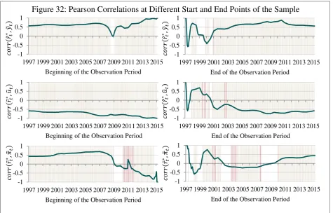
3.2.2 Correlation Analysis ... 30
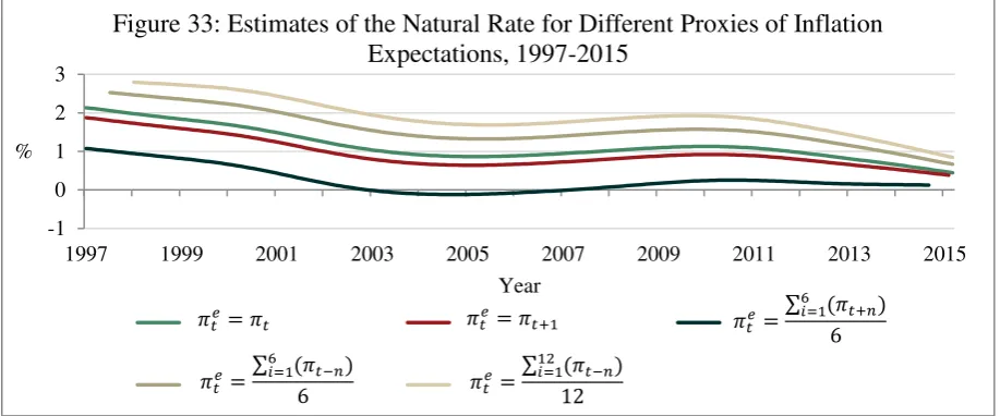
3.2.3 Sensitivity to the Assumption made on Inflation Expectations ... 37
3.3 Additional Considerations on the Natural Real Rate and Secular Stagnation ... 39
3.3.1 Overaccumulation in the Eurozone ... 39
3.3.2 Secular Stagnation and the Importance of Land ... 42
4. Secular Stagnation in the Long-Term Perspective ... 46
4.1 The Long-Term Challenge from Gordon’s Headwinds ... 46
4.1.1 Demographics ... 46
4.1.2 Education ... 48
4.1.3 Inequality ... 51
4.1.4 Government Debt ... 54
ii
5 Monetary Policy and the Decline of the Natural Rate of Interest ... 65
5.1 Identifying the ‘Correct’ Target Rate for the Eurozone ... 65
5.2 When One Size does not fit All: The Role of Diversity within the Eurozone ... 68
5.2.1 Target Rates, Policy Stress and Convergence at the Aggregated Group Level . 68 5.2.2 Target Rates, Policy Stress and Convergence at the Individual Country Level 72 5.3 Lessons from the USA ... 77
6 The Political Economics of a Reform ... 83
6.1 The Need for a Reform of the Fiscal and Monetary Framework ... 83
6.2 The Tragedy of the Euro ... 90
7 Conclusion and Recommendation for Further Research ... 101
iii List of Figures
Figure 1 Change in GDP and GDP per Capita for Major Developed Economies ... 4
Figure 2 Change in Imports and Exports for Major Developed Economies ... 5
Figure 3 GDP Growth Rates for Major Developed Economies ... 5
Figure 4 Secular Stagnation in the Loanable Funds Model ... 7
Figure 5 Investment-to-GDP Ratios for Major Developed Economies ... 8
Figure 6 Change in Unemployment and Youth Unemployment Rates for Major Developed Economies ... 9
Figure 7 Working Age Population Growth Rates for Major Developed Economies ... 9
Figure 8 Nominal Interest Rates and Core Inflation Rates for Major Developed Economies ... 10
Figure 9 Time-Varying Natural Rate for the USA ... 11
Figure 10 Potential GDP Estimates for the USA ... 11
Figure 11 Change in GDP per Capita in the Eurozone ... 13
Figure 12 Potential GDP Estimates for the Eurozone ... 13
Figure 13 Domestic Credit to the Private Sector in the Eurozone ... 14
Figure 14 Working Age Population Growth Rates for the Eurozone ... 15
Figure 15 Life Expectancy and Effective Retirement Age in the Eurozone ... 16
Figure 16 Income Inequality in the Eurozone... 16
Figure 17 Income Distribution in the Eurozone by Quintile ... 17
Figure 18 Material Deprivation and Risk of Poverty in the Eurozone ... 17
Figure 19 The Declining Relative Price of Investment in the Eurozone ... 18
Figure 20 Estimates of the Natural Rate of Interest for the Eurozone ... 20
Figure 21 Variables used for Estimating the Natural Real Rate ... 22
Figure 22 Core Inflation in New Zealand and the Eurozone ... 23
Figure 23 Time-Varying Natural Rate for the Eurozone ... 24
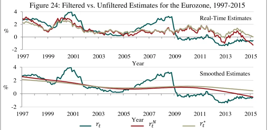
Figure 24 Filtered vs. Unfiltered Estimates for the Eurozone ... 25
Figure 25 Real Interest Rate Gap in the Eurozone ... 26
Figure 26 The Threat of Secular Stagnation in the Eurozone (Author’s Estimates) ... 26
Figure 27 Comparison with Crespo Cuaresma et al., Natural Real Rate ... 28
Figure 28 Comparison with Bouis et al., Natural Real Rate ... 29
Figure 29 Comparison with Bouis et al., Real Rate Gap ... 29
Figure 30 The Threat of Secular Stagnation in the Eurozone (Bouis et al.) ... 30
Figure 31 Variables used in the Correlation Analysis ... 32
Figure 32 Pearson Correlations at Different Start and End Points of the Sample ... 37
Figure 33 Estimates of the Natural Rate for Different Proxies of Inflation Expectations ... 38
Figure 34 Estimates of the Real Interest Rate Gap for Different Proxies of Inflation Expectations ... 38
iv
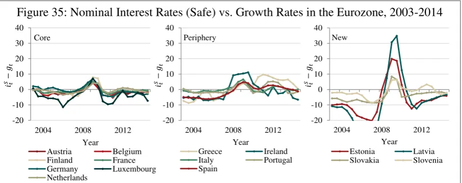
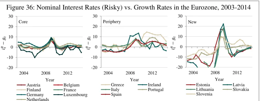
Figure 36 Nominal Interest Rates (Risky) vs. Growth Rates in the Eurozone ... 40
Figure 37 Weighted Average Cost of Capital vs. Growth Rates in the Eurozone ... 41
Figure 38 Values of Land, Capital, and Public Debt in the OECD ... 43
Figure 39 Value of Land in the OECD ... 43
Figure 40 Dependency Ratios in the Eurozone in 2015, 2030, and 2060 ... 46
Figure 41 Annual Growth Rates of Productivity Indicators in the Eurozone ... 47
Figure 42 Secondary and Tertiary Enrollment Ratios in the Eurozone ... 48
Figure 43 Private Costs of Attaining Tertiary Education in the OECD ... 50
Figure 44 Market Value of Private Capital in Europe and the World ... 52
Figure 45 Home Price Indices vs. Disposable Household Income in the Eurozone ... 53
Figure 46 Debt-to-GDP Ratios in the Eurozone and the United States ... 54
Figure 47 Government Debt and GDP Growth in the Eurozone, Pre-Crisis vs. Post-Crisis ... 55
Figure 48 Government Debt and Credit Rating in the Eurozone, Pre-Crisis vs. Post-Crisis ... 56
Figure 49 Average Growth in TFP and Real Value Added per Hour Worked in the USA ... 58
Figure 50 Number of Applications at the Largest Patent Offices ... 59
Figure 51 R&D as a Share of GDP ... 60
Figure 52 Number of Researchers per 1,000 Labor Force... 60
Figure 53 Tertiary Enrollment Ratios for the Different World Regions ... 61
Figure 54 World Population vs. Student Population ... 61
Figure 55 The Eurozone’s Share in Global Patent Applications ... 62
Figure 56 IPR and Subscores in the Eurozone ... 63
Figure 57 Taylor Rule Recommendations and MRO Rate ... 66
Figure 58 Taylor Rule Recommendations at Different Levels of the Natural Rate ... 67
Figure 59 Core Inflation, Output Gaps, and Unemployment Gaps in the Eurozone, Pre-Crisis vs Post-Crisis ... 68
Figure 60 Taylor Rule Recommendations at the Aggregated Group Level ... 69
Figure 61 Monetary Policy ‘Stress’ at the Aggregated Group Level ... 70
Figure 62 Taylor Rule Recommendations at the Individual Country Level ... 73
Figure 63 Monetary Policy ‘Stress’ at the Individual Country Level ... 74
Figure 64 Output Gaps and Unemployment Gaps in the USA and the Eurozone ... 79
Figure 65 Taylor Rule Recommendations and Monetary Policy ‘Stress’ in the USA ... 80
Figure 66 Compliance with the Deficit Criterion and the Debt Criterion ... 84
Figure 67 TARGET2 Balances for the Core and Periphery Countries ... 87
v List of Tables
Table 1 The Natural Real Rate of Interest and Monetary Policy ... 6
Table 2 Statistical Properties of the Variables used in the Correlation Analysis ... 32
Table 3 Main Results of the Correlation Analysis ... 32
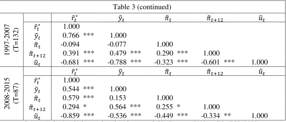
Table 4 Correlation between 𝑟̃𝑡∗ and 𝜋̃𝑡+𝑘 at Different Values of k ... 34
Table 5 The Real Rate Gap as a Predictor of Future Inflation ... 34
Table 6 Repeating the Correlation Analysis on the Estimates of Bouis et al. ... 35
Table 7 Tuition Fees & Financial Aid to Students in 2010, Eurozone vs. USA ... 50
vi List of Abbreviations
BEA Bureau of Economic Analysis
BLS Bureau of Labor Statistics
BMF Bundesministerium der Finanzen, Federal Ministry of Finance (Germany)
bn Billion
BoJ Bank of Japan
CeN Central and Northern European Currency (Hypothetical)
e.g. Exempli gratia, for example
EAPP Expanded Asset Purchasing Programme
ECB European Central Bank
EDP Excessive Deficit Procedure
EFSF European Financial Stability Facility
EFSI European Fund for Strategic Investment
EIB European Investment Bank
EMU Economic and Monetary Union
EPO European Patent Association
ESM European Stability Mechanism
EU European Union
EUFTA European Free Trade Agreement (Hypothetical)
et al. Et alii, and others
Fed Federal Reserve System
FRBSF Federal Reserve Bank of San Francisco
GDP Gross Domestic Product
GFS Government Financial Statistics
HP Hodrick-Prescott
i.e. Id est, that is to say
IMF International Monetary Fund
ISA Interdistrict Settlement Account
IT Information Technology
MRO Main Refinancing Operations
n.a. Not available
NAIRU Non-Accelerating Inflation Rate of Unemployment
OCA Optimum Currency Area
OECD Organization for Economic Co-Operation and Development
OLS Ordinary Least Squares
Pop. Population
PPP Purchasing Power Parity
PRA Property Rights Alliance
vii
R&D Research and Development
SD Standard Deviation
SGP Stability and Growth Pact
SNA System of National Accounts
R.o.W. Rest of the World
TARGET Trans-European Automated Real-Time Gross Settlement Express Transfer
System
TFEU Treaty on the Functioning of the European Union
TFP Total Factor Productivity
UK United Kingdom
UN United Nations
USA United States of America
WACC Weighted Average Cost of Capital
WIPO World Intellectual Property Organization
viii List of Symbols
𝑔 GDP growth rate
𝐼 Demand for loanable funds
𝑖𝑆 Short-term (3 month) nominal interest rate
𝑖𝐿 Long-term nominal interest rate
𝑖𝑀𝑅𝑂 Main refinancing operations rate
𝑖𝑅 Risky nominal interest rate
𝑖𝑇 Taylor rate
𝑖𝑊𝐴𝐶𝐶 Weighted average cost of capital (WACC) rate
𝑖̇̅𝑆 Average short-term (3 month) nominal interest rate
𝑖̇̅𝐿 Average long-term nominal interest rate
𝑘 Time lag factor
𝑛 Number of observations
𝑝 Value of significance
𝑟 Real interest rate
𝑟𝑁 Natural real interest rate (unfiltered)
𝑟∗ Natural real interest rate (filtered)
𝑟̃𝑁 Real interest rate gap (unfiltered)
𝑟̃∗ Real interest rate gap (filtered)
𝑠 Monetary policy ‘stress’
𝑆 Supply of loanable funds
𝑡 Observation Period
𝑇 Number of observation periods
𝑢 Unemployment rate
𝑢∗ Non-accelerating inflation rate of unemployment (NAIRU)
𝑢̃ Unemployment gap
𝑦 (Logarithm of) GDP
𝑦∗ (Logarithm of) Potential GDP
𝑦̃ Output gap (as % of GDP)
𝛼 Yield curve spread (term premium)
𝛽, 𝛿 Intercept, if subscript =0. Regression coefficient, if subscript >0.
𝜀, 𝜍 Error term
𝜆 Smoothing parameter
𝜋 Inflation rate (year-on-year)
𝜋𝑒 Expected inflation rate (year-on-year)
𝜋𝑇 Inflation target
ix
𝜏 Trend component
∗, † Level of significance (*** 0.1%, ** 1%, * 5%, † 10%)
1 1. Introduction
1.1 Problem Statement
When the global financial crisis reached its peak seven years ago, the Western world entered
what is known today as the ‘Great Recession’: A prolonged period of slow growth whose
impact is still painfully felt in many economies. While the academic world struggled to explain the unusually slow recovery from the crisis, Lawrence Summers (2014a) added a new
momentum to the debate when he reintroduced Hansen’s (1938) ‘secular stagnation’ hypothesis. According to this theory, the ‘natural’ real rate of interest (the rate which equates savings and investment under full employment) may have become negative in some Western
economies. If the inflation rate is low and the nominal interest rate – which is restricted by the
zero lower bound – cannot be lowered further, this would prevent conventional monetary
policy from adequately stimulating demand and, hence, economic growth. The economy could then fall into a self-enforcing era of economic stagnation unless bold monetary and fiscal stimuli and far-reaching structural reforms are implemented.
While an academic consensus on the occurrence of secular stagnation has yet to be reached, many observers agree that the Eurozone is much more susceptible to this threat than any other Western economy (with the possible exception of Japan). In most of its member countries, levels of GDP per capita are still lower than they were before the crisis. Rates of inflation and economic growth remain low despite nominal interest rates close to the zero lower bound. Levels of public debt and unemployment, on the other hand, have reached
alarming levels. In addition to that, large differences among the Eurozone’s member states
complicate the implementation of adequate monetary and fiscal policies to counter these developments. Because of this, a vibrant debate has recently emerged on whether the Eurozone might suffer from secular stagnation as defined by Summers (2014a).
However, while many scholars argue that the Eurozone’s natural real rate of interest might
have become negative, their proposals often remain largely theoretical and lack sufficient empirical backing. The present analysis aims to fill this gap by delivering a contemporary
estimate of the Eurozone’s natural real rate. Doing so will deliver two important contributions
to the debate on secular stagnation. Firstly, a comparison of this result with the ‘actual’ real
rate and the inflation rate will allow for a formal test of the occurrence of secular stagnation in the Eurozone. And secondly, as the natural real rate is an important determinant in the
monetary policy rule defined by Taylor (1993), the author’s estimates may also be used as a benchmark for assessing whether the ECB’s single monetary policy constitutes an adequate
ill-2
equipped to counter this threat, the present analysis will additionally aim at identifying appropriate monetary and fiscal policy measures.
While the empirical estimation of the Eurozone’s natural real rate should be regarded as the main contribution of the present analysis, the threat of secular stagnation will also be investigated under alternative definitions. Some scholars have argued that, even if the Eurozone should not be subject to a persistently negative natural real rate, it might still be threatened by secular stagnation if the latter is defined as a long-term decrease of potential output growth per capita. Gordon (2012) has proposed that such a decrease might be triggered
by a number of ‘headwinds’ (such as a decline in working-age population growth), and authors such as Kasparov and Thiel (2012) consider a slowdown of technological growth as a likely cause. Hence, in order to investigate the threat of secular stagnation in the Eurozone in its entire magnitude, these alternative definitions are tested as well.
Based on these considerations, the present paper aims at bringing some clarity to the vivid debate on secular stagnation. Specifically, the following research questions will be addressed:
1. Does the Eurozone face a serious threat from secular stagnation
a. in the short to medium term due to a decline in the natural real rate of interest?
b. in the long run due to a number of ‘headwinds’ or slow technological growth?
2. What are the implications of a declining natural real rate for the Eurozone’s
monetary policy?
3. To what extent is the Eurozone’s monetary and fiscal policy affected by the large
degree of diversity among its members?
4. Can the Eurozone’s economic outlook be improved by means of monetary and/or fiscal reform?
1.2 Structure of the Analysis
After this first section has defined the objective and primary research questions of the present paper, the subsequent analysis is structured as follows. Section 2 delivers an overview of
Summers’ (2014a) secular stagnation hypothesis and explains how this theory is linked to shifts in the natural rate of interest. An investigation of the main drivers of the natural rate shows why the threat of secular stagnation is often regarded as particularly acute in the case of the Eurozone. Based on these considerations, Section 3 offers a contemporary estimate for
the Eurozone’s natural real rate and a subsequent discussion of the implications for the threat of secular stagnation. The adequacy of these results is underlined by a variety of robustness
3 Section 4 investigates whether the Eurozone is likely to experience a long-term decrease of
potential output growth per capita due to Gordon’s (2012) headwinds or a slowdown in
technological growth. Section 5 assesses the appropriateness of the ECB’s single monetary
policy against the background of a declining natural rate. The analysis is conducted for the Eurozone as a whole as well as on the aggregated group level and the individual country level.
The term ‘diversity stagnation’ is coined in order to define the primary weakness of the Eurozone’s monetary framework. Based on these findings, Section 6 additionally highlights
the shortcomings of the Eurozone’s fiscal policies and investigates whether the Eurozone
could benefit from a far-reaching reform of its monetary and fiscal framework. Several possible scenarios are presented, and the likelihood of their implementation is discussed by
means of the theorem of the ‘tragedy of the commons’. Section 7 concludes the analysis and
delivers recommendations for future research.
Throughout the paper, many of the Eurozone’s most important macroeconomic
developments are analyzed in detail. As these developments often strongly vary among its 19 different member countries, it was deemed necessary to aggregate them into adequate country groups. Accordingly, the following arrangement has been maintained in the remainder of the
analysis. The Core group contains the long-term members whose economies have been rather
successful in overcoming the financial crisis and the Great Recession. The Periphery group
includes the long-term members who experienced the most significant economic hardships
during these periods. Finally, the New group consists of those members who consecutively
acceded to the Eurozone following the year 2007. An exception has been made for Cyprus: while it became a member country in 2008, it was deemed to be rather comparable to the
countries of the Periphery. Hence, the three groups were organized as follows:
The Core group: Austria, Belgium, Finland, France, Germany, Luxembourg
and the Netherlands
The Periphery group: Cyprus, Greece, Ireland, Italy, Spain and Portugal
4
Figure 1: Change in GDP and GDP per Capita for Major Developed Economies (Index = 2007), 2000-2019
80 90 100 110 120
2000 2005 2010 2015
%
Year GDP
Canada Japan Scandinavia United Kingdom United States Eurozone
80 90 100 110 120
2000 2005 2010 2015
%
Year GDP per Capita
2. The Threat of Secular Stagnation in the Eurozone 2.1 The Great Recession and Weak Economic Recovery
From the year 2007 onwards, the unfolding of the US subprime mortgage crisis and the global financial crisis paved the way for a significant decline in the world economy. However, the impact of this decline was unequally felt across the globe. While many developing and
emerging countries – most notably India and China – saw their economic growth largely
unimpaired, most Western economies experienced the worst financial crisis since the Great Depression (Stiglitz 2010). Consequently, in order to depict the analogy to the global crisis of the 1930s, the resembling downturn of our time has been labelled the ‘Great Recession’.1
Figure 1 illustrates its impact on economic growth in the developed world:2
Source: Author’s calculations; based on data provided by the IMF (2015)
Not only did the economies displayed in Figure 1 experience a significant contraction following the year 2007, but their growth rates also remained low after the initial decline was overcome. As a result, it took all of these economies several years to reach their pre-crisis level of economic performance. Canada experienced the fastest economic recovery, as its
1 While it has become common among academics and the media to refer to the aftermath of the financial crisis
as the Great Recession, it has to be noted that the term is not always used synonymously. In its academic sense, a recession only refers to the contraction phase of a business cycle (Claessens, Kose and Terrones 2009). As such, the Great Recession lasted from 2007 to 2009 in the case of the USA (and similarly for many other Western countries) and was a true global recession only in the year 2009 (IMF 2009). On the other hand, a wide range of authors define the Great Recession more broadly as the time period during which the impact of the global financial crisis continued to weight on the Western economies. According to this logic, the Great Recession lasted much longer and might still be ongoing, as many economic hardships continue to persist in the aftermath of the actual contraction. As these hardships are particularly felt in the Eurozone (as will be shown in Section 2.3), the present analysis defines the Great Recession in its broad sense as the time period since the global financial crisis.
2 Estimations start after 2011 for the United Kingdom, after 2012 for the United States and after 2013 for the
remaining countries. Scandinavia is defined in its strictest sense and hence only consists of Denmark,
5 GDP reached the pre-crisis level in the year 2010. The remaining economies did not achieve this task until the years 2011 (Eurozone and USA), 2012 (Scandinavia), 2013 (Japan) and 2014 (United Kingdom). The recovery required even more time in the case of GDP per
capita – as of 2015, three major economies (the Eurozone, Scandinavia, and the United
Kingdom) have not yet reached their respective pre-crisis level.
The significant reduction in economic performance reflects unfavorable developments in most economic indicators, such as an increase in unemployment and a decrease in investment and international trade. As shown by Figure 2, the value of goods traded by the Western economies experienced a much larger decrease than their GDP and GDP per capita. Post-crisis growth was low as well, and many of those economies still traded less in 2014
compared to 2007:3
Source: Author’s calculations; based on data provided by UN Comtrade (2015) and the St. Louis Fed (2015)
Many economists expressed astonishment regarding the recovery of most Western economies, which was widely considered as unusually slow even after allowing for the severe impact of the financial crisis (Goodwin et al. 2013). While severe recessions had taken place in the preceding decades as well, the same economies had always resumed their pre-crisis growth rates after a much shorter period of time:
Source: Author’s illustration; based on data provided by the OECD (2015)
3 The trade flows include the total of all HS commodities. All values were initially expressed in current US$
and have been adjusted using data on headline inflation provided by the Federal Reserve Bank of St.
Louis (2015). A detailed analysis of this “mystery of the missing world trade growth” is provided by
Armelius, Belfrage and Stenbacka (2014).
40 60
80
100 120 140
2000 2002 2004 2006 2008 2010 2012 2014
%
Year Value of Imports
Canada Japan Scandinavia United Kingdom USA Eurozone
Figure 2: Change in Imports and Exports for Major Developed Economies (Index = 2007), 2000-2014
40 60 80 100 120 140
2000 2002 2004 2006 2008 2010 2012 2014
%
Year
Value of Exports
Figure 3: GDP Growth Rates for Major Developed Economies, 1960-2015
-10 -5 0 5 10 15
1960 1970 1980 1990 2000 2010 %
Year
Growth rate compared to the same quarter of the previous year, seasonally adjusted
Canada Japan Scandinavia United Kingdom United States Eurozone -10
-5 0 5 10 15
1960 1970 1980 1990 2000 2010 %
6
Figure 3 highlights a number of earlier recessions, such as the 1970s energy crisis or the recessions of the 1980s and 1990s. In all of these cases, economic growth in the Western economies recovered relatively fast, often even surpassing pre-crisis growth rates after a short time. This illustrates the severity of the Great Recession in a historical context and justifies the analogy with the Great Depression of the 1930s. But Figure 3 also delivers a second important insight: for most Western economies, average growth has continuously declined during the previous decades. Eight years after the global financial crisis, these economies seemingly remain trapped within an equilibrium of slow growth.
2.2 The Secular Stagnation Hypothesis and its Recent Popularity
Against this background, Summers (2014a) expressed the concern that Western economies
might suffer from more profound constraints than just from a ‘normal’ cycle of slow growth. Referring to a theory formulated by Hansen (1938), he reintroduced the term ‘secular stagnation’ in order to describe what he considered as a long-term decline in the potential of Western economies. This theory is intrinsically tied to developments in the natural real rate of interest introduced by Wicksell (1898), which equates savings and investment under full
employment.4 The difference between the natural real rate and the real rate of interest (the
nominal rate of interest minus the inflation rate) determines to which degree the central
bank’s monetary policy stimulates the economy. Table 1 highlights how the relationship
between real rate 𝑟 and natural real rate 𝑟∗ influences an economy’s inflation gap (𝜋̃), output
gap (𝑦̃), and unemployment gap (𝑢̃):5
Table 1: The Natural Real Rate of Interest and Monetary Policy
𝑟 = 𝑟∗ 𝑟 < 𝑟∗ 𝑟 > 𝑟∗
𝜋̃ 0 ↑ ↓
𝑦̃ 0 ↑ ↓
𝑢̃ 0 ↓ ↑
Source: Woodford (2003)
Only if the real rate corresponds to the natural real rate, the economy operates at potential. In this case, inflation is at target and the output and unemployment gaps are closed. If the real rate falls short of the natural real rate, the result is an increase in inflation and output gap, and
4 The natural rate is also known by a variety of other names, such as equilibrium rate, neutral rate, or
Wicksellian rate. While all of these designations are common in the prevalent literature, this analysis only refers to it as the natural (real) rate of interest.
5 The inflation gap is defined as actual inflation minus the inflation target. The output gap is specified as GDP
7
vice versa (Woodford 2003).6 As the natural real rate is not directly observable, the central
bank has to rely on estimations when deciding upon the optimum policy rate.7 Within this
setting, Summers (2014a) formulated his (new) secular stagnation hypothesis. He argues that a chronic excess of savings over investment (or, to put it differently, a prolonged shortfall in aggregate demand) cannot be reversed by conventional monetary policy if the natural real rate of interest has become significantly negative, trapping the economy in a state of sluggish
growth. This problem can be illustrated by a simple loanable funds model:8
Source: Author’s illustration following Krugman (2000) and Summers (2014a)
Let I and S denote the demand for investment and the supply of savings at full
employment. Furthermore, r is the real interest rate, r* is the natural real interest rate and π is
the inflation rate. In Figure 4a, I and S intersect in the positive area and r* is significantly
larger than 0. If r* and π are correctly estimated by the central bank, it can set a nominal
interest rate which equates savings and investment at full employment. In Figure 4b, the
demand for investment decreases – triggered, for instance, by a decline in the working age
population or by a lack of profitable investment opportunities. If the decrease is large enough,
it is possible that I and S now intersect in the negative area. The result is a negative r*, but as
it is still located above the inverted inflation rate, it can be targeted by the central bank as
well. But if investment demand falls even further, the economy can enter a situation where r*
lies below the inverted inflation rate (see Figure 4c). As the nominal interest rate is
6 Woodford (2003) dedicates an entire chapter of his work to an analysis of the natural rate of interest in the
context of monetary policy. He shows how “increases in output gaps and in inflation result from increases in
the natural rate of interest that are not offset by a corresponding tightening of monetary policy […], or
alternatively from loosenings of monetary policy that are not justified by declines in the natural rate of interest.” He does not mention the unemployment gap, but due to the tradeoff between unemployment and losses in a country’s GDP (Okun 1962), this variable was included nevertheless.
7 However, as will be further elaborated in Section 3, estimates of the natural rate are surrounded by a high
degree of uncertainty.
8 While emanating from different considerations, the secular stagnation hypothesis shares many features with
the ‘liquidity trap’ hypothesis, such as the focus on low inflation and the zero lower bound on nominal interest rates. The similarity of both concepts has also been acknowledged by Krugman (2013, 2014). For this reason, Figure 4 is based on the notation used in Krugman (2000). A more in-depth representation of secular stagnation using the loanable funds model has been provided by Eggertsson and Mehrotra (2014).
Figure 4: Secular Stagnation in the Loanable Funds Model
r
I, S r*
-π
S I
0
r
I, S r*
-π
S I
0
r
I, S
-π
S
I
0
r*
8
constrained by the zero lower bound (ZLB), there is no achievable real interest rate which equates savings and investment at full employment. Hence, conventional monetary policy cannot provide sufficient stimulus to elevate the economy from a state of low demand. Economic growth remains sluggish and the economy will continue to operate below potential,
leading to disinflation and leaving output and unemployment gap open. This is what
Summers (2014a) defines as secular stagnation.9
The reintroduction of the secular stagnation theory by Summers (2014a) has been met with widespread recognition, as many scholars regard it as a comprehensible explanation for the
weak performance of most Western economies.10 A vivid debate has emerged on the optimum
policy response, as only unconventional measures – such as raising inflation (expectations)
through quantitative easing (QE) or boosting demand through expansionary fiscal policy –
may lift an economy from a state of secular stagnation (Duprat 2015). In this analysis, it is
argued that the sudden rise of the theory’s popularity can be explained by at least four factors.
Firstly, the global financial crisis has indeed resulted in a tremendous decline in the Western
countries’ demand for investment, as illustrated in Figure 5:
Source: Author’s illustration; based on data provided by the IMF (2015) and the World Bank (2015)
9 However, it has to be recognized that the term ‘secular stagnation’ is not always used synonymously – as
Eichengreen (2014) put it, “Secular Stagnation […] is an economist’s Rorschach test. It can mean different things to different people.” In the prevalent literature, there exist at least two interpretations of secular stagnation apart from the one provided by Hansen-Summers. The first one defines secular stagnation as a
long-term decrease in potential output growth due to a number of ‘headwinds’. This interpretation is
delivered by Gordon (2012), who argues for the existence of six ‘headwinds’ (in Gordon 2014, he reduces
the number to four – demographics, education, inequality, and government debt). The second interpretation
focuses on the inhibitive effect of balance sheet recessions on economic growth. Authors such as Koo (2011, 2014) and Lo and Rogoff (2015) argue that unsustainable levels of debt in the years leading to the financial crisis have triggered an extensive process of deleveraging, and that economic growth will remain sluggish as long as this process prevails. While the three different interpretations share many common characteristics, they also differ in important aspects. A detailed comparison is provided by Pradhan et al. (2015), who also show that the three interpretations are mutually exclusive (the authors label this phenomenon as the “impossible trinity” of secular stagnation). In the present analysis, the term ‘secular stagnation’ is always used in the sense intended by Hansen (1938) and Summers (2014a) unless explicitly stated otherwise.
10 However, it has also received a significant degree of criticism, as will be laid out in Section 2.3.
Figure 5: Investment-to-GDP Ratios for Major Developed Economies, 1980-2015
10 15 20 25 30 35
1980 1985 1990 1995 2000 2005 2010 2015 %
Year
Gross Capital Formation (% of GDP)
Canada Japan Scandinavia United States United Kingdom Eurozone
10 15 20 25 30 35
1980 1985 1990 1995 2000 2005 2010 2015 %
Year
9 On average, the share of investment in GDP has dropped by 19.7% (gross capital formation) and 21.4% (total investment) between 2007 and 2009. As of 2015, Canada is the only economy where the ratios have reached their pre-crisis levels, and growth remains low in all of the economies. In a simple loanable funds model (see Figure 4), this would constitute a significant shift of the demand curve to the left.
Secondly, unfavorable developments in many of the drivers of investment demand – both
in the short and in the long run – indicate that aggregate demand may continue to grow at low
levels. As an example of a short-term development, Figure 6 displays the surge in unemployment following the financial crisis:
Source: Author’s illustration; based on data provided by the OECD (2015)
Beginning in the year 2008, all of the economies listed in Figure 6 experienced significant increases in their unemployment rates, especially in youth unemployment. While these rates have largely decreased between 2010 and 2015 (with the exception of the Eurozone, which saw a second increase following the beginning of the sovereign debt crisis), they still remain above the pre-crisis rates for all economies but Japan. As a contrast to the short-term increase in unemployment rates, Figure 7 presents the decline in working age population growth rates, which is a long-term evolution common to all major Western economies:
Source: Author’s illustration; based on data provided by the OECD (2015)
Figure 6: Change in Unemployment and Youth Unemployment Rates for Major Developed Economies, 2000-2015
0 5 10 15 20 25
2000 2002 2004 2006 2008 2010 2012 2014 %
Year Both sexes, aged 15-64
Canada Japan Scandinavia United Kingdom United States Eurozone
0 5 10 15 20 25
2000 2002 2004 2006 2008 2010 2012 2014 %
Year Both sexes, aged 15-24
-2 0 2 4
1950 1960 1970 1980 1990 2000 2010
%
Year Age 15-64 years, both sexes, Change from year ago
Canada Japan United Kingdom United States Scandinavia Eurozone
Figure 7: Working Age Population Growth Rates for Major Developed Economies, 1950-2013
-2 0 2 4
1950 1960 1970 1980 1990 2000 2010
%
10
As of 2013, the working age population was either declining or growing at very low levels
for all economies displayed above.11 As can be seen from the 5-year averages, this does not
represent a cyclical, but rather a truly secular development which is unlikely to be reversed in the near future. As demand for consumption and investment is primarily driven by the
working age population, higher unemployment rates12 and a decline in the working age
population growth indicate a lower growth of aggregate demand in the short and long run. Hence, both of these short- and long-term developments suggest that a significant shortfall of demand may require a long time to be reversed.
Thirdly, all major Western economies exhibit low inflation rates and even lower short-term
nominal interest rates, as illustrated by Figure 8:13
Source: Author’s illustration; based on data provided by the BoJ (2015), Eurostat (2015), the OECD (2015) and
the St. Louis Fed (2015)
After the onset of the Great Recession, short-term nominal rates were sharply reduced in all major Western economies. As of 2015, Canada and the United Kingdom display the highest rates, at 0.89% and 0.54%, respectively. The remaining economies have reduced their rates to levels close to the zero lower bound. Core inflation rates are low as well, amounting to 2.4% and 1.8% for Canada and the USA and to less than 1% for the remaining economies. As has been illustrated in Figure 4, low inflation coupled with nominal interest rates close to the zero lower bound may be problematic if the natural real rate declines. If actual real rates
11 In the case of the Eurozone, data for all current member countries has been aggregated (with the exception of
Cyprus, Malta, Latvia, and Lithuania). Each member country has been weighted according to the relative size of its population (as has also been done in the case of Scandinavia). In order not to distort the implications drawn from the trend growth line, the increase in working age population due to the German reunification is not reflected in Figure 7.
12 Higher unemployment leads to lower demand not only among the unemployed, but also among the employed
population, as those who still have a job reduce consumption and investment as well if they sense a higher degree of uncertainty on the labor market. Hence, the inhibitive effect of unemployment on growth may be much larger than indicated by the unemployment rate only.
13 As they do not form a monetary union, aggregating the Scandinavian countries’ interest and inflation rates
would deliver a misleading result. Therefore, these countries are not represented in Figure 8.
Figure 8: Nominal Interest Rates and Core Inflation Rates for Major Developed Economies, 1965-2015
-5 0 5 10 15 20 25
1970 1980 1990 2000 2010 %
Year
Short-Term Interest Rate
Canada Japan United Kingdom United States Eurozone -5
0 5 10 15 20 25
1970 1980 1990 2000 2010 %
Year
11 cannot be reduced to the level of a significantly negative natural real rate, conventional monetary policy may be deprived of its chances of stimulating the economy.
As has been shown so far, recent developments indicate that a decline in the natural real rate may have taken place in the Western countries, that such a development is unlikely to be reversed in the near future, and that these countries are ill-equipped to counter negative natural rates due to low inflation and the zero lower bound on nominal rates. A final factor in explaining the popularity of the secular stagnation hypothesis can be found in the detailed information available for the USA, especially concerning the development of the natural rate.
Figure 9 presents Laubach and Williams’ (2003) updated estimate of the natural rate.
According to these authors, the US-American natural real rate has experienced a continuous decline during the past 50 years and has even dropped into the negative territory after the onset of the Great Recession. When taking both the zero lower bound on nominal interest rates and low core inflation rates into account (see Figure 8), this signifies that a further decline in either the natural rate or the inflation rate would pose a threat of secular stagnation (see Figure 4).
Source: Laubach and Williams (2003) Source: Summers (2014b),,,
Summers (2014b) shows how this development coincided with a sequential downward
trend in the predictions made on the U.S. economy’s potential GDP (see Figure 10), which he considers as indicative for the inhibitive effect of a declining natural rate on economic
growth.14 Hence, the current experiences of the US-American economy seem to support the
secular stagnation hypothesis.
14 While it was estimated in the year 2007 that the economic potential would amount to almost 21 Trillion US$
in the year 2018, this estimate was since reduced to about 19.3 Trillion US$. Hence, Summers argues that the reduction in the US-American output gap has not been achieved by an increase in economic performance, but rather by a downward correction of its potential GDP.
Figure 10: Potential GDP Estimates for the USA, 2007-2017 Figure 9: Time-Varying Natural Rate
for the USA, 1965-2015
-2 0 2 4 6
1970 1980 1990 2000 2010 %
Year
One-Sided Estimates Two-Sided Estimates
15 16 17 18 19 20 21
2007 2009 2011 2013 2015 2017
T
rilli
on
s
of
2
01
3
$
Year
12
2.3 The Case of the Eurozone
The previous section has delivered an overview of the secular stagnation hypothesis
reintroduced by Summers (2014a). It has also been shown that the theory’s popularity can be
explained by the fact that it delivers a comprehensible – and seemingly empirically backed –
explanation to what is perceived as unsatisfactory performance and outlook in many developed economies. However, compliance with this view is not unanimous, and a number
of prominent economists – such as Bernanke (2015), Hamilton et al. (2015), Mokyr (2014a),
and Taylor (2014)15 – have argued against the case of secular stagnation. But while no
consensus has yet been reached on the threat of secular stagnation for the Western world as a
whole, there seems to be a rather strong agreement on a certain point – namely, that the
Eurozone is much more vulnerable than other developed economies.16 In the present section,
it will be investigated to what extent this presumption is justified.
To begin with, Figure 1 has already shown that the Eurozone’s recovery from the financial
crisis was much slower compared to most other Western economies. The impact of the Great
Recession – coupled with the sovereign debt crisis – continues to weigh heavily on many of
its members, particularly on the Periphery countries:
,,,,,,,,,,,,,
15 While all of these – and a number of other authors – reject the proposal of secular stagnation, they avail
themselves of very different arguments in doing so. Bernanke (2015) considers not a decline in aggregate
demand for investment, but rather a global increase in desired savings –the ‘savings glut’ – as causative for
weak economic growth. Within the loanable funds model (see Figure 4), this would translate into a rightward
shift of the S-curve instead of a leftward shift of the I-curve. Hamilton et al (2015) argue that a state of a low
(or even negative) natural real rate is not necessarily self-enforcing, and that the natural real rate may evolve back to a higher ‘normal’ level without the aid of extraordinary policy measures. Mokyr (2014a) brings forward that current technological progress (especially within fields such as nanotechnology, genetic engineering, and artificial intelligence) may lead to a boost in the productivity of Western economies. He
argues that the effects are widely underestimated today, since aggregate statistics such as GDP and TFP –
which “were designed for a steal and wheat economy” – do not properly capture productivity gains stemming from these fields. Finally, Taylor (2014) considers inefficient economic policies as the main reason for the financial crisis and the weak recovery of most Western economies. He puts forward that the market was deeply disrupted before the crisis by the Fed’s low interest policy and the loose enforcement of financial regulations as well as by a large number of policy measures which were implemented afterwards. He argues
that the financial crisis and the Great Recession – and, consequently, the fear of secular stagnation – would
have turned out less severe without these “deviations from rule-based policies that had worked in the past.”
16 Buiter, Rahbari and Seydl (2014) analyze the risk of secular stagnation for the Eurozone, Japan, the UK, the
USA, and a number of emerging markets and conclude that “the threat […] is probably most serious in the
Euro area”. Crafts (2014) regards the Eurozone as “much more vulnerable” to the threat of secular stagnation than the USA, concluding that the Europeans “should be much more afraid than the Americans”. While they consider most of the developed world to be in danger of secular stagnation, Posen and Ubide (2014) argue that the Eurozone “has made that situation worse for itself” by means of counterproductive policy measures.
And Duprat (2015) considers the Eurozone “not well equipped to manage the challenge” and identifies a real
13 Source: Author’s calculations; based on data provided by the IMF (2015)
The New country group experienced the fastest recovery from the financial crisis: as of 2015, only Slovenia has yet to reach its pre-crisis level of GDP per capita. The developments were less favorable in the Core countries, as five out of seven countries have not yet reached their pre-crisis level and growth remains low in all countries except Germany. But these economic hardships seem to fade when compared to those of the Periphery group, whose members all display significantly lower GDP per capita levels compared to 2007. In fact, the IMF (2015) expects that the recovery will take until the year 2018 in the case of Portugal and Spain, and much longer for the remaining countries in this group.
This evidence illustrates that slow economic growth is not only significant for the Eurozone as a whole, but that its 19 member countries have been subject to the economic hardships following the financial crisis to a strongly varying degree. This distinct heterogeneity (which will be addressed more explicitly in Section 5) is one of the (many) reasons for which the Eurozone is often seen as particularly vulnerable towards secular stagnation. First evidence on this threat came from Summers (2014b) himself, who has shown
that the Eurozone’s economic performance was not only far below its potential during recent
years, but that its potential GDP has also continuously been corrected downwards:
Source: Summers (2014b)
8 8.5 9 9.5 10 10.5 11
2007 2008 2009 2010 2011 2012 2013 2014 2015 2016 2017
T rilli on s of 2 00 5 E ur os Year
Figure 12: Potential GDP Estimates for the Eurozone, 2007-2017
Actual GDP 2008 Estimate 2010 Estimate 2012 Estimate 2014 Estimate
60 80 100 120 140
2000 2005 2010 2015 % Year Core Austria Belgium Finland France Germany Luxembourg Netherlands Eurozone 60 80 100 120 140
2000 2005 2010 2015 % Year Periphery Cyprus Greece Ireland Italy Portugal Spain Eurozone 60 80 100 120 140
2000 2005 2010 2015 % Year New Estonia Latvia Malta Slovakia Slovenia Lithuania Eurozone
14
In the year 2008, the IMF and Bloomberg databases (on which Summers 2014b bases his
illustration) expected the Eurozone’s potential GDP to reach more than 10.5 trillion euros by the year 2017 (measured in 2005 euros). This estimate was consecutively reduced to less than
9.5 trillion euros, which will probably still be much larger than the Eurozone’s actual GDP in
the year 2017. According to Summers (2014b), this large decrease in the monetary union’s
economic potential cannot only be explained by the aftermath of the global financial crisis,
but is likely to reflect a long-term decline in the natural real rate.17 In the following, it will be
examined whether such a decline may indeed have occurred. According to the formal model provided by Eggertsson and Mehrotra (2014), four factors are primarily accountable for such a decline: (1) a deleveraging shock, (2) a slowdown in population growth, (3) an increase in
income inequality, and (4) a fall in the relative price of investment.18
A deleveraging shock takes place if the simultaneous deleveraging effort of a significant
number of economic entities – either in the private sector, the public sector, or both – creates
adverse effects for the country’s economic activity. In the case of some Eurozone countries,
rapid credit expansion in the years leading to the financial crisis resulted in unsustainable levels of debt in the non-financial private sector (Cuerpo et al. 2014). After the financial crisis and the onset of the Great Recession, this resulted in a significant deleveraging shock in these
member countries:19
Source: Author’s calculations; based on data provided by the World Bank (2015)
17 As has taken place in the USA, see Figures 9 and 10.
18 There are certainly a number of additional factors playing a role as well. For instance, Eichengreen (2015)
considers the global integration of emerging markets as a major reason for an increase in savings and a decrease in investment demand. And Andréz, López-Salido and Nelson (2009) show how the natural real rate can be driven down by a technology shock. For the sake of feasibility, however, this analysis considers only the primary factors which have been identified by Eggertsson and Mehrotra (2014).
19 Initially, the World Bank’s (2015) measure of domestic credit to the private sector was expressed as % of
GDP, with levels ranging from 41.1% (Lithuania) to 252.5% (Cyprus) in the year 2014.
Figure 13: Domestic Credit to the Private Sector in the Eurozone (Index = 2007), 1990-2014
0 50 100 150 200
1990 1995 2000 2005 2010 %
Year Core
Austria Belgium
Finland France
Germany Luxembourg
Netherlands Eurozone
0 50 100 150 200
1990 1995 2000 2005 2010 %
Year Periphery
Cyprus Greece
Ireland Italy
Portugal Spain
Eurozone
0 50 100 150 200
1990 1995 2000 2005 2010 %
Year New
Estonia Lithuania
Latvia Malta
Slovakia Slovenia
15 As can be seen from Figure 13, the percentage increase in domestic credit in the years leading to the financial crisis was particularly large for the Periphery countries and the New countries (except Slovakia), but also for some Core countries (such as Finland and the Netherlands). Most Eurozone countries (14 out of 19) experienced private sector deleveraging between 2007 and 2014. The percentage change was particularly large (above 20%) in the case of Belgium, Estonia, Germany, Ireland, Latvia, Lithuania, Malta, Slovenia and Spain. Since private sector deleveraging shocks translate into a significant reduction of consumption and investment (Cuerpo et al. 2014), it can be assumed that this development has exerted
considerable downward pressure on the Eurozone’s natural rate of interest.
Concerning the slowdown in population growth (the second factor mentioned by
Eggertsson and Mehrotra 2014), Figure 7 has already illustrated that the Eurozone’s working
age population was growing slower than those of Canada, Scandinavia, the United Kingdom and the United States. The severity of this development is further illustrated by Figure 14, which delivers the growth rate in the population aged 15 to 64 for each Eurozone country. It is found that most member countries are currently experiencing a long-term decline in their growth rate, which can roughly be traced back until the 1980s. As of 2013 only Italy, Luxembourg, and Portugal recorded a positive growth in their working age population (and in the case of Italy and Portugal, this seems to have represented a cyclical deviation from the significant decline which they had recorded in the preceding years):
Source: Author’s calculations; based on data provided by the World Bank (2015)
As has been laid out in Section 2.2, the decline in the working age population growth indicates a lower growth of aggregate demand for loanable funds in the long term. For the Eurozone, this is further exacerbated by the increasing discrepancy between life expectancy
and retirement age, as can be seen from Figure 15:20
20 In each of the three different country groups, the respective member countries have been weighted according
to their relative size of their GDP in each year. If information on GDP was not available for a given year,
Figure 14: Working Age Population Growth Rates for the Eurozone, 1955-2013
16
Source: Author’s calculations; based on data provided by the OECD (2012) and the UN (2013)
For each group of countries, the life expectancy of both the male and the female population experienced a considerable increase during the last four decades. At the same time, the average effective retirement age was continuously reduced until about 1995 and has remained low until 2012. As a result, the gap between both indicators has widened in almost every year since 1970. This means that the average worker now spends a larger percentage of his lifetime being a retiree and a smaller percentage belonging to the working age population. Similar to the decrease in working age population growth, this development can be expected to reduce demand for investment and consumption, leading to a decline in the natural rate of interest.
While these demographic factors highlight unfavorable developments in almost all member countries, the case of income inequality (the third factor mentioned by Eggertsson and Mehrotra 2014) delivers a more differentiated picture. Figure 16 illustrates the income ratio of the richest quintile relative to the poorest quintile for each Eurozone country:
Source: Author’s calculations; based on data provided by Eurostat (2015)
As can be seen from Figure 16, income inequality strongly varies among the different country groups. Most Periphery countries demonstrate a much higher inequality compared to the Core countries, and the three Baltic states are far more unequal than the remaining countries in the New group. The development between 2007 and 2013/14 displayed simple averages were calculated instead. Comparative tests have shown that doing so did not significantly alter the results. Unless stated otherwise, the same procedure has been chosen for all subsequent charts.
Figure 15: Life Expectancy and Effective Retirement Age in the Eurozone, 1970-2012
55 60 65 70 75 80 85
1970 1980 1990 2000 2010
A
ge
Year Male Population
Life Expectancy - Core Effective Retirement Age - Core Life Expectancy - Periphery Effective Retirement Age - Periphery Life Expectancy - New Effective Retirement Age - New
55 60 65 70 75 80 85
1970 1980 1990 2000 2010
A
ge
Year Female Population
Figure 16: Income Inequality in the Eurozone, 2000-2014
3 4 5 6 7 8
2000 2004 2008 2012
S8 0/S2 0 R atio Year Core Austria Belgium Finland France Germany Luxembourg Netherlands Eurozone 3 4 5 6 7 8
2000 2004 2008 2012
S8 0/S2 0 R atio Year Periphery Cyprus Greece Ireland Italy Portugal Spain Eurozone 3 4 5 6 7 8
2000 2004 2008 2012
17 significant differences between the countries as well, as inequality decreased in five member countries (Germany, Ireland, Netherlands, Portugal, and Finland) and remained at a comparable level for two additional member countries (Belgium and Estonia). In the remaining countries, however, the income distribution became more unequal. As a result, the inequality increased by 3.6% between 2007 and 2013 for the Eurozone as a whole (and by 18.9% from 2000 to 2013). Further detail on this development is provided by Figure 17. Between 2000 and 2013, the Eurozone experienced not only a decrease in the share of national income held by the first quintile, but also a decrease in the share held by the second, third, and fourth quintile (albeit to a lesser extent). Only the share held by the fifth quintile
increased significantly. Hence, it can be taken that the Eurozone’s income distribution has
continuously become more unequal during the most recent years. And, as noted by Eggertsson and Mehrotra (2014), such a development may have a negative impact on the aggregate
demand for investment and hence reduce the natural real rate of interest.21
In addition to that, a higher degree of income inequality has often been found to be associated with a higher risk of poverty and an increase of material deprivation (see, for instance, Lelkes et al. 2009 and Calvert and Nolan 2012). As shown in Figure 18, the risk of poverty has increased in 15 out of 19 member countries since the global financial crisis. The material deprivation rate has increased in 12 countries. If households are exposed to a higher risk of poverty, this translates into a lower demand for investment and consumption (especially among risk-averse agents). Similarly, as the material deprivation rate reflects the
21 Specifically, Eggertsson and Mehrotra (2014) distinguish between two types of income equality which may
put downward pressure on the natural real rate: inequality within generations and inequality across
generations. Information on the Eurozone’s income distribution across different age groups can be obtained
from Eurostat (2015). However, this data is only available for the years 2005-2014, which was deemed insufficient for adequately investigating changes in intergenerational distributions. As a result, the present analysis only focuses on inequality within generations.
0 5 10 15 20 25 L atv ia Gr ee ce C yp ru s L ith uan ia Italy Po rtu gal Sl ov ak ia Ir elan d Ma lta Est on ia Sl ov en ia Sp ain Ger m an y B elg iu m Fra nce Au str ia Fi nlan d Neth er lan ds L ux em bo ur g %
Risk of Poverty 2007 Risk of Poverty 2013
Material Deprivation Rate 2007 Material Deprivation Rate 2013 0 10 20 30 40 1st Quintile 2nd Quintile 3rd Quintile 4th Quintile 5th Quintile %
2000 2005 2010 2013
Figure 17: Income Distribution in the
Eurozone by Quintile, 2000-2013 Figure 18: Material Deprivation and Risk of Poverty in the Eurozone, 2007 vs. 2013
Source: Author’s illustration; based on data
18
“inability to afford a selection of items that are considered to be necessary or desirable”
(Eurostat 2015), such as not being able to finance a car, an increase in this rate reflects a reduction in investment demand. Therefore, it can be concluded that the economic consequences of increased income inequality have recently led to a downward pressure on the
Eurozone’s natural rate of interest.
Finally, Eggertsson and Mehrotra (2014) argue that a decline in the relative price of investment represents the fourth major reason for a decline in the natural rate of interest. According to this rationale, a lower relative price of investment (for instance, due to productivity gains owed to advances in information technology and the computer age) reduces the required savings rate, as less savings are needed for building the same stock of capital (Karabarbounis and Neiman 2014). This in turn drives down the natural rate of interest. Figure 19 highlights the decline in the relative price of investment within the Eurozone:
Source: Artus (2015)
As can be seen from Figure 19a, the relative price of productive investment (e.g., investment in information technology) has been reduced by almost 20% during the last two decades. The reduction in the relative price of investment led to falling prices and higher productivity in the sectors which produce capital goods and IT products, as illustrated in Figure 19b. Per capita productivity has significantly increased in both sectors, but even more so in the IT sector (which also was much less affected by the financial crisis). Figure 19c shows that the nominal investment rate has been falling relative to the real investment rate since the year 1995, with both rates coinciding in the year 2006. This implies that a given growth in GDP and capital in real terms could be achieved with a smaller nominal capital stock (Artus 2015). Therefore, it can be assumed that the fall in the relative price of
investment – just as the three factors analyzed before – has led to a reduction of the demand
for loanable funds, resulting in downward pressure on the Eurozone’s natural rate.
Figure 19: The Declining Relative Price of Investment in the Eurozone, 1995-2015
80 85 90 95 100
1995 2000 2005 2010 2015 %
Year Figure XXXa
Productive Investment Deflator/ GDP Deflator (Index = 1995)
Productive Investment Deflator/GDP Deflator
40 60 80 100 120
1995 2000 2005 2010 2015
1,0
00
€
Year Figure XXXb
Per Capita Productivity, Capital Goods Sector vs. IT Sector
Capital Goods Sector IT Sector
7 8 9 10 11 12
1995 2000 2005 2010 2015 %
Year Figure XXXc
Productive Investment as a Share of GDP
% of Real GDP % of Nominal GDP
19 The present section has highlighted the thread of secular stagnation in the Eurozone based on the remarks of Eggertsson and Mehrotra (2014), who argue that four factors may be causative for a decline in the natural rate of interest. It was shown that, in recent years, the Eurozone has been subject to unfavorable developments in all four of these factors. It is
therefore concluded that the Eurozone’s natural rate is likely to have declined, which is an
essential prerequisite for secular stagnation as defined by Summers (2014a). Based on these
considerations, Section 3 provides a detailed assessment of the Eurozone’s natural real rate in
20
3 The Natural Real Rate and Secular Stagnation in the Eurozone 3.1 A Contemporary Estimate of the Eurozone’s Natural Real Rate 3.1.1 Existing Studies
As has been laid out in Section 2.2, Summers’ (2014a, 2014b) definition of secular stagnation
is intrinsically tied to developments in the natural real rate of interest. Specifically, a decline in the natural real rate coupled with low inflation rates may prevent the real rate of interest from becoming sufficiently negative (given the ZLB as a lower limit for the nominal rate of interest) to drive the real rate gap below zero. Hence, secular stagnation is formally defined as a permanently positive real rate gap coupled with low inflation (Pedersen 2015). It follows that, in order to draw conclusions on the presence of secular stagnation in the Eurozone, a contemporary estimate of the natural real rate is required.
Unfortunately, the natural real rate is not directly observable, and its estimation is surrounded by a high degree of complexity and uncertainty. So far, no consensus has been reached on the optimum methodology, and a number of scholars have offered different estimations of the natural real rate for the Eurozone. Commonly applied methods were, among others, multivariate structural time series models (Crespo Cuaresma, Gnan, and Ritzberger-Gruenwald 2004), consumption-based capital asset pricing models (Browne and
Everett 2005), as well as variants of Laubach and Williams’ (2003) Kalman filter approach
(Garnier and Wilhelmsen 2005, Benati and Vitale 2007, Mésonnier and Renne 2007).
Figure 20 summarizes the findings of these studies:
Source: Benati & Vitale (2007), Browne & Everett (2007), Crespo Cuaresma et al. (2004), Garnier & Wilhelmsen (2005), Mésonnier & Renne (2007), Eurostat (2015), and OECD (2015)
Unfortunately, all of these studies offer estimates of the natural real rate only until the year 2005 (with initial years ranging from 1965 to 1999), and one would certainly assume that significant shifts have occurred since then (see Section 2.3). Nevertheless, Figure 20 is useful
0 1 2 3 4 5
1995 1996 1997 1998 1999 2000 2001 2002 2003 2004 2005
%
Year
Figure 20: Estimates of the Natural Rate of Interest for the Eurozone, 1995-2005
Real Interest Rate Crespo Cuaresma et al.
Benati & Vitale Garnier & Wilhelmsen