Commonality and Heterogeneity in Real Effective Exchange Rates: Evidence from Advanced and Developing Countries

Munich Personal RePEc Archive

Commonality and Heterogeneity in Real

Effective Exchange Rates: Evidence from

Advanced and Developing Countries

Nagayasu, Jun

1 March 2016

Online at

https://mpra.ub.uni-muenchen.de/70078/

Commonality and Heterogeneity in Real Effective

Exchange Rates: Evidence from Advanced and

Developing Countries

∗

Jun Nagayasu

Abstract

In order to differentiate between commonality and heterogeneity in real effective exchange rates, which are considered a measure of external competitiveness, we de-compose their movements into global and country-specific factors using the Bayesian factor model. First, we show a complex but often positive relationship between real exchange rates and net trade volume using panel data of developed and developing countries. Then we report a particular global trend in real exchange rates, but a substantial proportion of their variation is found to be country-specific. In line with this finding, we conclude that structural shifts, when they do exist, are considered country-specific factors. Furthermore, consistent with economic theory, this global factor is closely related to a trend in the global interest rate, while country-specific factors are closely related to idiosyncratic movements in the countries’ own inter-est rates. Such a decomposition results in better model performance in terms of coefficient signs, and therefore our results suggest that external competitiveness is heterogeneous among countries and that economic policy can influence countries competitiveness.

Keywords: Real effective exchange rates, factor model, variance decomposition, external competitiveness

JEL classification: F31

∗_{This research was carried out when the author was visiting the University of Strathclyde and the} University of Glasgow (UK). I would like to thank Miguel Belmonte, Julia Darby, Ronald MacDonald, and Stuart McIntyre for providing me with an excellent research environment. Also thanks for helpful dis-cussions and Takeshi Hoshikawa, Eiji Ogawa, Junko Shimizu, Naoyuki Yoshino and other participants in biannual meetings of the Japanese Economic Association and the Japan Society for Monetary Economics. The research was funded by a Grant-in-Aid for Scientific Research (C) No 25380386.

1

Introduction

Co-movements in exchange rates have been analysed in several contexts. Co-movements,

which can be measured by the sensitivity of one currency to another in regression analysis

or by the simple correlation coefficient, are important since changes in one currency indeed

often affect the currency of other countries (e.g. McKinnon and Schnabl (2003)),

particu-larly those with a flexible exchange rate regime. Furthermore, currency interdependence

has been examined in the context of inferring actual exchange rate regimes which may be

deviating from officially announced ones (e.g. Frankel and Wei (2008)).

Co-movements in exchange rates are also underlined during financial crises;

deterio-ration in one’s currency value almost simultaneously affects others through, for example,

speculative attacks (e.g. Gerlach and Smets (1995), Masson (1998)). Such an effect is

often called contagion in the academic literature and has become increasingly prominent

in recent years when a series of financial crises affected the world economy. Such crises

include the 1997 Asian crisis which erupted in Thailand, the Lehman Shock (2008) in the

United States, and the European sovereign debt crisis which started in Greece (2009).

Each crisis led the original country’s economy and the regional and/or world economy

into recession.

The majority of previous studies on co-movements seem to have investigated

common-ality in stock prices; furthermore, those on foreign exchange markets have focused largely

on bilateral nominal exchange rates (see the abovementioned literature and the next

sec-tion). However, foreign exchange transactions are conducted in a global context with the

involvement of more than two countries. Furthermore, researchers and policymakers are

certainly interested in studying real effective exchange rates which are often regarded as

an economic variable for measuring the external competitiveness of countries (e.g.

UNC-TAD (2012), Brixiova (2013)), and are considered, at least on theoretical grounds, as

one important factor contributing to economic growth. Indeed, a number of empirical

research projects have been conducted in order to investigate whether undervalued

cur-rencies bring about economic growth (e.g. Bhalla (2008), Rodrik (2008), Mbaye (2012),

UNCTAD (2012), Brixiova (2013), Levy-Yeyati et al. (2013)).1

1

Against this background, this study analyses and quantifies co-movements in real

effec-tive exchange rates for a wide range of countries. There must be some level of correlation

in these rates as they are affected by developments in international economies. However

given that competitive and non-competitive countries co-exist in the global market, it

would be of interest to researchers and policymakers to quantify the level of the rates’

co-movements and determinants. We analyse the determinants based on previous studies

which, without data decomposition, have used real interest rates to explain bilateral real

exchange rates. Early studies tend to cast doubt on the credibility of this relationship

for individual exchange rates (Edison and Pauls (1993), Edison and Melick (1999)), for

example, based on the lack of cointegration and/or the wrong coefficient signs for real

interest rates. However, stronger evidence in favor of this relationship has been reported

by more recent studies (MacDonald and Nagayasu (2000), Byrne and Nagayasu (2010))

in the panel data context.

A distinguishing feature of this study is that real effective exchange rates are

de-composed for a more comprehensive number of countries into global and country-specific

factors using a Bayesian factor model. (The number of countries under investigation in

previous studies seems often rather limited i.e., fewer than 15 countries, as summarised

in Section 4.) The Bayesian model allows us to estimate a more comprehensive definition

of global movements.2

The decomposition into global and country-specific factors is also

conducted for the driving forces of exchange rates. By doing so, we can estimate ‘foreign’

variables which are often assumed to be the U.S. data in previous studies. In this way,

our statistical model departs from those of previous studies on bilateral exchange rates

and becomes more congruent with economic theory and data.3

definition of external competitiveness.

2

However, over the last decade much progress has been made in estimating commonalities in large data sets, especially studies on business cycles (Forni et al. (2000), Kose et al. (2003), Foerster et al. (2011)) and general commodity (non-financial asset) inflation (Bernanke et al. (2005), Canova and Ciccarelli (2009), Mumtaz and Surico (2012))

3

2

Driving forces behind real effective exchange rates

What are the driving forces behind real effective exchange rates? Among others, economic

theory suggests that real exchange rates are determined by the real interest rate

differen-tial or the productivity differendifferen-tial in tradable sectors (known as the Balassa-Samuelson

theorem). Here we use real interest rates which are available for more countries, and

summarise their theoretical link, following Obstfeld and Rogoff (1996). Their derivation

of the model is more general than the conventional one using solely the purchasing power

parity (PPP) theorem and the uncovered interest rate parity (UIRP) condition, in the

sense that sticky prices are considered in the model.

Let us consider domestic inflation which can be explained by the Dornbusch-type

inflation specification for an open economy:

∆pt+1 =γ(y_td−y_t) + ∆st+1+ ∆˜p∗_t+1 (1)

where yd

t is the demand for home country output, s is the nominal effective exchange

rate and p is the price. All variables are in log form, and ∆ represents the differenced

operator; therefore, ∆pt+1 =pt+1−ptbecomes inflation. A variable with a bar indicates a

natural level, and a foreign variable is denoted with an asterisk. In the presence of multiple

partner countries, the latter can be thought of as a weighted average of foreign variables

suggested by the tilde in Eq. (1). The γ >0 implies that home inflation increases due to

excessive demand for home products, exchange rate depreciation, and increases in foreign

inflation. In such cases, there is no market clearance, that is, ∆pt+1 6= 0.

Further, the demand for home products (yd

t) is assumed to be expressed as:

y_td= ¯yt+δ(st−pt+ ˜p∗

t −q¯) (2)

where δ > 0. As in the previous studies, the long-run (or natural) real exchange rate

(¯q) is assumed to be fixed here. According to Eq. (2), the demand for domestic goods

exceeds its natural level to an extent proportional to the level of currency misalignment.

Using the definition of the real exchange rate (qt≡st−pt+˜p∗t) which suggests that gains

in external competitiveness are shown as increases in qt, and the UIRP (∆st+1 =it−˜i∗_t

∆pt+1 =γδ(qt−q¯) +it−˜i∗t + ∆˜p∗t+1 (3)

In addition, using the Fisher condition (it =Rt+ ∆pe

t+1 where Rt is the real interest

rate and a variable with superscript e indicates an expected value) and rearranging Eq.

(3) in term of the real exchange rate, we can obtain the following relationship:

qt= ¯qt− 1

δγ(Rt−R˜

∗

t) (4)

Sinceγandδare theoretically positive, this equation asserts that there would be home

currency depreciation when the real interest rate falls at home. Eq. (4) is an appropriate

theoretical framework even when a country is confronted with very low nominal interest

rates since real interest rates can be negative owing to the presence of expected inflation.

However, as mentioned, previous studies (e.g. Edison and Pauls (1993)) often report

wrong parameter signs for real interest rates. For the estimation, we consider the equation

of exchange rate changes which is consistent with an a priori assumption of the standard

factor model:

∆qt=− 1

δγ∆Rt+

1 δγ∆ ˜R

∗

t (5)

We base our empirical analysis on Eq. (5): since there are two components (global

and country-specific factors) in real effective exchange rates, each factor is estimated by

real interest rates. The global factor in real effective exchange rates is expected to be

de-termined by the global interest rate ( ˜R∗

t), and the country-specific factor by idiosyncratic

movements in the interest rates (Rt).

3

Data and preliminary analyses

Real effective exchange rate (Q) data are obtained from the International Financial

Statis-tics (IFS) of the International Monetary Fund. They (IFS code: ..REUZF, 2005 = 100)

are constructed using the consumer price indices (CPI) and weights determined by the

size of trade (unit values) to each trading partner, and cover the sample period from

(see Table 1). The country coverage and the sample period are determined by data

avail-ability from the IFS and maximise the total number of observations.4

In the subsequent

analysis, we analyse exchange rate growth, that is, the first difference of log exchange

rates (ln(Qt/Qt−1)), in order to be congruent with an a priori assumption of the data

required for the factor model.

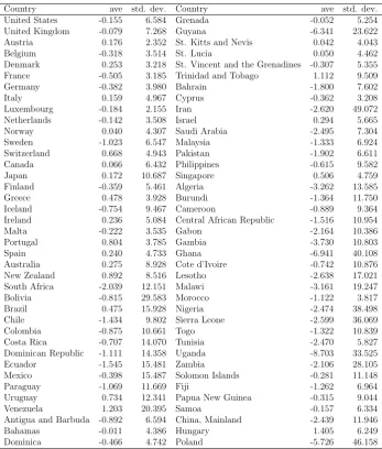
The basic statistics of the exchange rates are summarised in Table 2. The sign of the

average (ave) exchange rates suggests that the direction of exchange rate movements is

diversified, and almost three-quarters (72 percent) of the countries have experienced a

fall in exchange rates (Table 2). Furthermore, developing countries have experienced a

higher level of exchange rate volatility than advanced countries, measured by the standard

deviation (std. dev.). This outcome seems to be closely associated with the deterioration

in domestic economies; for example, Poland was confronted with accelerating inflation

from the late 1980s to the early 1990s.

Table 1 also provides information about the data required to calculate real interest

rates, which we obtain on the basis of the Fisher hypothesis (real interest rates = nominal

interest rates expected inflation rates). Here, nominal interest rates are either the market

rates or deposit rates, and as a proxy for expected inflation we assume ex ante inflation

using the CPI.5

Data availability for the interest rate and CPI reduces the number of

countries to 17, for which there are sufficient time-series data for statistical analysis; most

of the countries are advanced countries.

The time-series properties of real exchange rates and interest rates are examined by

panel unit root tests. In order to examine the null hypothesis of non-stationary data,

we implement two types of tests, namely, the Levin-Lin-Chu (LLC, (2002)) and

Fisher-type (Choi (2001)) tests. In order to take into account cross-sectional dependence, the

LLC statistic is obtained by removing the cross-sectional mean from the original data

prior to the test. The second test is based on the work of Fisher (1932) who proposed

poolingp-values from independent tests in order to create a statistic which can be used to

assess unit roots in the panel data context. Furthermore, following Choi (2001), different

specifications of the latter test are used. Table 3 reports strong evidence of a stationary

4

The other definition of real effective exchange rates is available from the IFS. However, the country coverage for the alternative rates is much narrower than that based on the CPI.

5

process for changes in both real exchange rates and interest rates; the null is rejected at

the one percent significance level in favor of the alternative of stationarity. Although our

data are effective rates, the stationarity of differenced exchange rates is consistent with

previous studies on bilateral exchange rates which have achieved the stationarity after

taking the first difference (Hallwood and MacDonald (2000)).

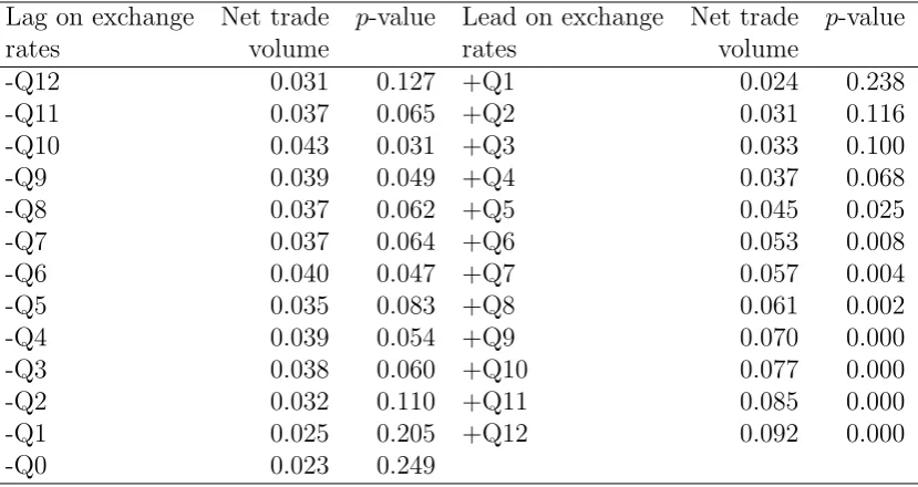
While our analysis focuses on the real exchange rate-interest rate relationship, real

exchange rates are often discussed as related to international trade at least in theory.

Therefore, as part of our preliminary analyses, we calculate the correlation coefficients

between real effective exchange rates and net trade volume.6

Since their causality remains

questionable (e.g. McKenzie (1999), Barkoulas et al. (2002)), we conduct this exercise for

two cases where real exchange rates affect previous and future trade volumes (Table 4).

Our statistical results show the complex nature of this relationship7

: we discover a link

between exchange rates and international trade, but the degree of statistical significance

depends on the gestation periods (i.e. a lead or lag length) during which exchange rates

(the trade balance) are thought to influence the trade balance (exchange rates). Notably,

we often obtain evidence of the expected outcome, that is, a positive correlation between

exchange rates and net trade volume, and in line with the conventional economic theory

(e.g. the J-effect) there is a time lag (slightly more than one year) for them to influence

one another statistically significantly. This shows why real effective exchange rates have

often been considered a measure of external competitiveness.

4

Empirics

There are several statistical approaches to analyzing co-movements in data. The

tradi-tional, and probably most popular, approach is to use correlation measures between data.

Increased correlation is regarded as evidence of increased cross-country linkages, and high

correlation during tranquil times with minimal risk premia is also interpreted as evidence

of high capital market integration. Such research can be carried out either by simply

calculating correlation coefficients among financial data or estimating the exchange rate

6

The trade data are also obtained from the IFS.

7

equation of one country with other countries’ exchange rates as explanatory variables.

Based on this approach, previous studies have pointed out unstable interrelationships

and increased correlation at times of financial crises in equity markets (Longin and Solnik

(1995), Reinhart and Carvo (1996), Liu et al. (1998), Bayoumi et al. (2007)). However,

there are potential problems with this estimation approach. Obviously, the

regression-based approach requires an exogeneity assumption about explanatory variables, but it

may be difficult to justify this assumption using volatile financial asset data.

Further-more, Forbes and Rigobon (2002) argued that the standard regression analysis fails to

take into account market volatility which differs during crisis and non-crisis periods.

Alternatively, co-movements can be estimated using a factor model or a principal

components approach. The factor model is often used to distinguish between global and

country-specific elements, and according to this approach, increases in the proportion of

the global factor become evidence of higher cross-country linkages (Koedijk and Schotman

(1989), Dungey (1999), Cayen et al. (2010)). The commonality in the data can also be

estimated by the principal components approach. For example, Nellis (1982) analysed

financial market integration using corporate and government bonds with the expectation

that their yields will be dominated by common factors in a highly integrated financial

market. Similarly, Volosovych (2013) studied financial market integration utilizing

gov-ernment bond yields from 1875 to 2009 and provided evidence of increased integration

from the data through the end of the 20th century. However, the coverage of these studies

is rather limited – often less than 15 countries – even when the factor/principal

compo-nents approach is used.

This study follows the second strand of the literature (i.e., the factor model) in which

all variables are treated as endogenous and which is thus more suitable for obtaining

global factors from a large number of countries. We now explain the statistical method

used to identify the number of common factors.

4.1

Identifying the number of common factors

Are there any common movements in real effective exchange rates and real interest rates?

This section details our investigation, which involves identifying the number of common

the factor model has been widely used in previous studies, the identification of the number

of common factors has remained a big challenge for researchers.

The statistical approach of Alessi et al. (2010) is an extension to Bai and Ng (BN,

(2002)), and thus is based on a factor model which for stationary data (x_nt =x1t, ..., xnt)′

is often expressed as:

x_nt =Λ_nF_t+e_nt, where t= 1, . . . , T (6)

where the data are standardized. Ft is a k×1 vector of common factors, and Λn is

a corresponding factor loading matrix (n×k), where k (k < min (n, T)) represents the

number of common factors. Since the size of loadings can differ among n, ΛnFt can be

viewed as common elements which include heterogeneous responses of each country (n)

to common movements (Ft). The residual (ent) which cannot be explained by F, is

con-sidered as idiosyncratic factors, and as in the standard model, common and idiosyncratic

factors are assumed to be orthogonal. In our research setting, x becomes a vector of

changes in real effective exchange rates or real interest rates.

While there are several statistical methods such as the Scree Plot to decide the

appro-priate number of common factors, recently a number of information criterion-type (IC)

methods have been proposed by BN (2001). However, while BN provides several forms of

penalty functions, the numerical simulations suggest that their estimation criteria tend to

under- or over-estimate the true number of common factors (Alessi et al. (2010)). Thus

we use a statistical method introduced by Alessi et al. (2010), who modified the BN

criteria by introducing the extra term (c∈ ℜ+

) to the penalty function.

IC(k) : min

0≤r∗≤k ln(V(k, ˆ

Fk)) +ckg(n, T) (7)

where V(.) = (nT)−1Pn

i=1

PT

t=1(xnt −ΛknFkt) 2

. A penalty factor g(n, T) will make

adjustments to the statistics for over-fitting in order to avoid cases where the solution is

always equal to k =n−1. More concretely, the large (small) crepresents over-(under-)

penalization, and when c= 0, it means no penalization. Furthermore, for a given k, the

appropriate number of common factors (r∗_{) corresponds to minimisation of the sum of}

information about the number of common factors although this extra term does not affect

the asymptotic performance in identifying the size of r∗_{. In that sense, their modification}

may seem trivial, but it has been shown to significantly influence the outcome with finite

data (Alessi et al. (2010)).

Alessi et al. (2010) also argued that r∗ _{should not be sensitive to the size of c. Thus}

once r∗

is obtained, we shall check its stability by means of the Sc statistic:

Sc = 1

J J

X

j=1

"

r∗

− 1

J J

X

h=1 r∗

h

#2

(8)

As Eq. (8) suggests, a small Sc implies the stability of r∗ since Sc approaches zero

when r∗ _{converges to the average of its own previous values. Thus, according to Eq.}

(8), r∗ _{should be chosen when S}

c approaches zero, and Alessi et al. (2010) proposed a

graphical approach to evaluate it.

Our estimates forr∗ _andS

c are shown over a range ofcin Figure 1. They are obtained

with k = 5 for a set of real effective exchange rates and real interest rates, and we show

that there is one common factor in both data. When several stability interval periods

exist, we choose the second long interval following the practical guidance of Alessi et al.

(2010). Thus Figure 1 seems to suggest that there is one common factor in a set of 78

real effective exchange rates and that of 17 real interest rates. We consider the former as

the global movements in real effective exchange rates and the latter as the global interest

rate (i.e., ˜R∗

t in Eq. (5)). The global interest rate has been discussed by a number

of researchers; for example, the high correlation of real interest rates among advanced

countries has been documented by Cumby and Mishkin (1986), Goodwin and Grennes

(1994), Gagnon and Unferth (1995), and Monadjemi (1997), and the close relationship

between advanced and emerging markets by Chinn and Frankel (1995).

4.2

Estimating global and country-specific factors

Given evidence of the global (common) factor found in the analysis in the previous section,

this study uses the factor model in order to calculate the size of this factor in our data.

Several researchers have applied the Bayesian approach to the factor model in finance

the arbitrage pricing theory (APT) in the context of the Bayesian framework, which

allows us to estimate a more complicated model than the Maximum Likelihood (ML)

approach. We follow their approach to estimate the factor model withFt∼N(0,Ik) and

e_t ∼N(0,Σ) in Eq.(6).

Apart from the number of common factors (r∗_{), one needs to deal with an identification}

issue. In particular, the number of parameters estimable has to meet the condition that

n ≥ 2r∗_{+ 1 (Geweke and Zhou (1996)) since the covariance matrix v is related with Λ}

and Σ through v = Λ′_Λ

+Σ, using the notation used to explain Eq. (6), where v has

n(n+ 1)/2 elements andΛ′_{Λ+Σ with nr}∗_{+n elements.}

Furthermore, given Λ is of full rank and the assumption that the first r∗

rows of

are independent,Λr∗ is a lower triangularr∗_×r∗ _{matrix with positive diagonal elements}

(Λ_ii>0 where i= 1, ..., r∗

):

Λr∗ =

       

Λ11 0 · · · 0

Λ21 Λ₂₂ · · · 0 ... ... . .. ... Λr∗1 Λr∗₂ · · · Λr∗r∗

        (9)

We estimate Eq. (6) using the Bayesian approach with a prior distribution; as Λij is

normal with a zero mean for i6=j, the likelihood function becomes

p(x|F,Λ,Σ)∝ |Σ|−T /2

exp (trace(−0.5Σ−1e′e)) (10)

This equation will be used to draw observations for parameters (b∗

i) in the Gibbs sampling

method for i= 1, ..., r∗ _as:

f(b∗

i|F, σi)∝exp

− 1

2σ2 i

(b∗

i −ˆb∗i)′F

′

iFi(b∗i −ˆb∗i)

(11)

where ˆb∗

i is the OLS estimate (b∗i = (Λi1, ,Λii)), andF_i contains the first r∗ elements

of F. b∗

i is independently normally distributed. Furthermore, the diagonal elements of Σ

follow the inverted gamma distribution:

f(σi|F,b∗i)∝ 1 σv+1

i

exp

−vs2 i 2σ2

i

where s2

i =T−

1PT

t=1e

′_{e and v =T. Geweke and Zhou (1996) explained that vs}2 i/σ

2 i

equivalently follows the χ2

(T) distribution, and when F and x are jointly normally

dis-tributed, the conditional value of Fand the covariance matrix can be shown as:

E(Ft|Λ,Σ,xt) = Λ

′

(ΛΛ′ +Σ)−1 xt

Cov(Ft|Λ,Σ,xt) = I−Λ

′

(ΛΛ′ +Σ)−1 Λ

(13)

The choice of prior distributions is always a challenge in Bayesian statistics, but those

assigned to the parameters here are the standard ones often employed in applied research

in economics and finance (Koop (2003)). Our results from the Gibbs sampling method are

based on 10,500 replications with 500 burn-in observations, which seem to be adequate

to achieve convergence.

One way to show the estimated global and idiosyncratic factors is to present their

contribution to the overall variation. Thus, the significance of common and

country-specific factors is analysed using the variance decomposition method (Table 5). Our

results suggest that a large portion (about 70 to 8 percent) of a variation in real effective

exchange rates is attributable to the country-specific elements, and is generally invariant

even if a different sample period and country coverage become research targets. Since

this is the first attempt to decompose real effective exchange rates, we cannot compare

our findings with previous ones. However, one interesting outcome of our study is that

advanced countries have experienced a higher proportion of country-specific movements,

implying relatively more heterogeneous responses of these countries to the recent financial

crises (the Lehman Shock (2008) and the Greek and European sovereign debt crises (2009

onwards)). In contrast, although it is not a significant difference, non-advanced countries

tend to follow more common movements after the Lehman Shock.

4.3

Characteristics of latent factors

Next, we analyse the characteristics of the global factor by checking if this factor is

persistent and contains a structural shift. If the characteristics are significant, we need

to incorporate them in subsequent analyses. First, whether or not the global factor is

persistent is examined by evaluating a fractional differencing parameter (d) which can

which often examine if data follow a stationary (d = 0) or unit root (d = 1) process.

Here we allow the possibility that ddoes not need to be exactly one of these two extreme

values. In that case the data can be shown to be stationary if−1/2< d < 1/2, and have

a long memory if 0< d < 1/2 (e.g. Granger and Joyeux (1980)).

We estimated the size of d for Ft, which is common across countries, by following

Geweke and Porter-Hudak (GPH, 1983) and Phillips (1999), who modified the GPH

method for nonstationary data by using the log periodogram regression. Our estimates

from these two methods are -0.047 [0.263] and -0.180 [0.269] respectively where the

num-bers in brackets are standard errors. Thus our estimates of d are not statistically

signif-icant, and provide evidence against the long memory of the global factors. Therefore, it

provides support for the specification of our factor model.

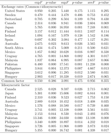
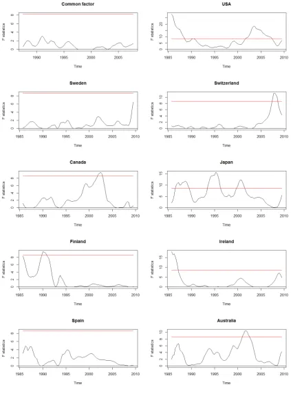
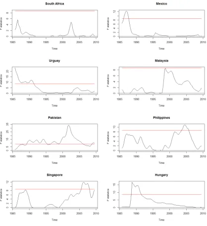
Furthermore, given the number of economic and financial crises during our sample

period, we also checked if global and country-specific factors contain a structural shift.

In line with this goal, three statistical tests were conducted to analyse the null

hypoth-esis of no structural breaks: the supF, aveF, and expF tests (Andrew (1993), Andrew

and Ploberger (1994)). They are popular approaches for detecting a structural shift in

stationary data utilizing F statistics obtained from shortened sample periods (discarding

the first and last 15 percent of observations). The large size of these statistics becomes

evidence of a structural shift in the data. In order to evaluate the statistical hypotheses,

p-values are calculated following Hansen (1997).

Our results suggest evidence of structural shifts in country-specific factors of real

effective exchange rates (Table 6, Figure 2); in contrast, there is no sign of structural

breaks in the common factor. Therefore, it appears that abnormal changes in external

competitiveness have been largely attributable to countries own economic responses. This

may be surprising because global financial crises have adverse impacts on many countries,

and thus one may expect to have structural shifts in the common factor in real effective

exchange rates. Again this result implies that heterogeneity in real effective exchange

5

Economic explanations of each factor

5.1

Country-specific factors

What would explain the country-specific factors in real effective exchange rates? Based

on our findings on the characteristics of data, we analyse this using idiosyncratic

com-ponents in real interest rates. Since the country-specific factors are supposed to be

in-dependent across countries, the mean group (MG) estimate approach which assumes no

cross-sectional dependence across countries, is used to understand the relationship

be-tween heterogeneity in country-specific real effective exchange rates and interest rates.

The MG is useful for obtaining the sensitivity of these two rates while taking into

ac-count heterogeneous sensitivities (slopes) among ac-countries (Pesaran and Smith (1995)).

We obtain the MG parameter for the panel data by averaging the parameters obtained

from individual country analyses. Furthermore, given that there are structural breaks in

our data, the specification of countries which have experienced structural breaks contain

a dummy variable. This dummy is equal to one after the breakpoint identified by the F

test (Figure 2) and to zero otherwise. The countries which did not exhibit a structural

break do not contain any dummy.

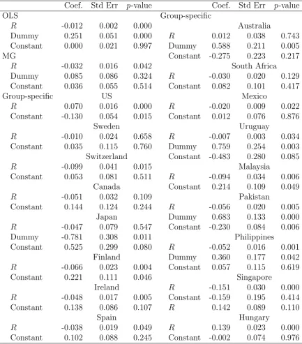
Table 7 summarises the results from the OLS and MG methods for the purposes of

comparison. The parameters of the real interest rates are of the most interest to us and

are reported to be negative and statistically significant, consistent with economic theory.

While the size and statistical significance of this parameter differ among countries, the

negative relationship between country-specific movements in real effective exchange rates

and interest rates is confirmed for the majority of countries.

5.2

Global factor

Similarly, we analyse the relationship between the global component in the real effective

exchange rates and the world real interest rates. The global factor (ΛnFt) differs among

countries, and, unlike country-specific factors, the elements in the global factor do not

suffer from structural breaks and are expected to be correlated across countries.

There-fore, in order to take into account the common time and country-specific effects in the

consistent estimates in the presence of cross-sectional dependence.

The estimation of the AMG consists of two steps; first, we obtain the time effects by

means of the following equation for the global factors of real exchange rates (x):

∆x_nt =b′_n∆z_nt+ct∆Dt+ent (14)

where xnt = ΛnFt and znt is a vector of the global factor of real interest rates. The

D is equal to one for a particular year and to zero otherwise, and this dummy can be

considered to capture the common factor in the global factor. The second step involves

the estimation of Eq. (15) using the common time effect obtained from Eq. (14):

xnt =b

′

nznt+cnµt+ent (15)

where µt = ˆct. These two steps are estimated by the OLS, and the slope for the panel

data can be calculated by ˜b =N−1PN

i=1bi (Eberhardt and Bond (2009)).

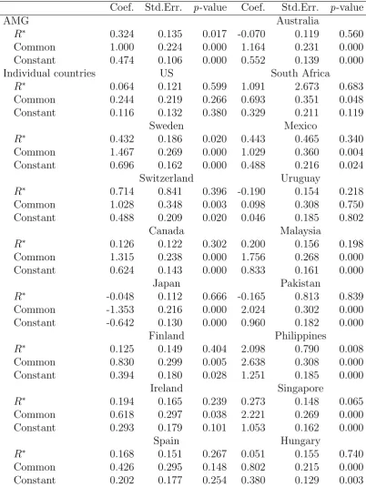
Table 8 summarises the results from the AMG and confirms in the panel context

the positive and significant relationship between the global factors in the real exchange

rates and the interest rates. This relationship is consistent with theoretical predictions

depicted in Eq. (5), and implies that a rise in the global interest rate (both R∗ _{and the}

common time effect (Common)) will increase home countries’ external competitiveness.

An individual country analysis provides somewhat weaker evidence for this relationship

because the parameter sign forR∗ _{is negative in four countries but it is the common time}

effect which influences the global factor of real exchange rates statistically significantly

and positively.

6

Conclusion

For a large group of countries, we have analysed if there is any common trend in real

effective exchange rates which can be regarded as a proxy for the external competitiveness

of countries. By decomposing exchange rates into global and country-specific factors using

a Bayesian factor model, we have confirmed that there is a unique trend in these rates.

losing or gaining external competitiveness simultaneously. The majority of movements in

real effective exchange rates are found to be idiosyncratic rather than common factors, and

this phenomenon is observed especially in advanced countries after the Lehman Shock.

These results imply that the external competitiveness of a country is rather heterogeneous,

and thus, a country which loses market competitiveness cannot solely blame external

factors for the loss.

The results of our further analysis suggest that this common trend can be explained by

the global interest rate computed by the factor model, and the country-specific movements

by the idiosyncratic movements in interest rate changes. Therefore, the degree to which

competitiveness has changed is largely determined by the countries’ economic policies.

This finding supplements that of Mbaye (2013), who confirmed a productivity channel in

economic growth; our results suggest that low real interest rates at home lead to increases

in real effective exchange rates that often have a positive relationship with net trade

volume, which measures part of general economic activities.

Our findings are in contrast to those of previous studies which have often reported

a poor relationship between exchange rates and interest rates (e.g. Edison and Pauls

(1993)). With regard to this relationship, recent studies point to the importance of

private information, carry trades, investors irrationality, and risk premia, among many

others (e.g., Evans and Lyons (2002)). While a direct comparison cannot be made between

studies on nominal and real exchange rates, our results which are more consistent with

theoretical predictions may be attributable to the consideration of low frequency data,

which, in turn, allow us to analyse the trend (rather than volatility) of real exchange rates

and the third-country effect, which has often been ignored in previous studies focusing on

References

Alessi, L., M. B. and M. Capasso (2010). Improved penalization for determining the number of factors in approximate factor models. Statistics and Probability Letters 80, 1806–1813.

Andrews, D. W. K. (1993). Tests for parameter instability and structural change with unknown change point. Econometrica 61 (4), 821–856.

Andrews, D. W. K. and W. Ploberger (1994). Optimal tests when a nuisance parameter is present only under the alternative. Econometrica 62(6), 1383–1414.

Bai, J. and S. Ng (2002). Determining the number of factors in approximate factor models.

Econometrica 70, 191–221.

Barkoulas, John T., C. F. B. and M. Caglayan (2002). Exchange rate effects on the volume and variability of trade flows. Journal of International Money and Finance 21, 481–496.

Bayoumi, T., G. Fazio, M. Kumar, and R. MacDonald (2007). Fatal attraction: Using distance to measure contagion in good times as well as bad. Review of Financial Economics 16(3), 259 – 273. Exchange Rates and International Financial Assets: A Special Issue in Honor of Stanley W. Black.

Bernanke, B., J. B. and P. S. Eliasz (2005). Measuring the effects of monetary policy: A factor-augmented vector autoregressive (FAVAR) approach. Quarterly Journal of Economics 120 (1), 387–422.

Bhalla, S. S. (2008). Economic development and the role of currency undervaluation.

Cato Journal 28, 313–340.

Brixiova, Z., B. Egert, and T. H. A. Essid (2013). The real exchange rate and external com-petitiveness in Egypt, Morocco and Tunisia. Working Paper 187, African Development Bank Group.

Byrne, J. P. and J. Nagayasu (2010). Structural breaks in the real exchange rate and real interest rate relationship. Global Finance Journal 21 (2), 138–151.

Calvo, S. and C. Reinhart (1996, June). Capital flows to Latin America : Is there evidence of contagion effects? Policy Research Working Paper Series 1619, The World Bank.

Canova, F. and M. Ciccarelli (2009). Estimating multicountry var models. International Economic Review 50 (3), 929–959.

Cayen, J.-P., D. Coletti, R. Lalonde, and P. Maier (2010). What drives exchange rates? new evidence from a panel of u.s. dollar bilateral exchange rates. Working Paper 2010-5, Bank of Canada.

Choi, I. (2001). Unit root tests for panel data. Journal of International Money and Finance 20, 249–272.

Cumby, R. E. and F. S. Mishkin (1986). The international linkage of real interest rates: the european-us connection. Journal of International Money and Finance 5(1), 5–23.

Dungey, M. (1999). Decomposing exchange rate volatility around the pacific rim. Journal of Asian Economics 10 (4), 525–535.

Eberhardt, M. and S. Bond (2009). Cross-section dependence in nonstationary panel models: a novel estimator. MPRA Paper 17870.

Edison, H. J. and W. R. Melick (1999). Alternative approaches to real exchange rates and real interest rates: three up and three down. International Journal of Finance & Economics 4(2), 93–111.

Edison, H. J. and B. D. Pauls (1993). A re-assessment of the relationship between real exchange rates and real interest rates: 19741990. Journal of Monetary Economics 31, 165–187.

Evans, M. D. and R. K. Lyons (2002). Order flow and exchange rate dynamics. Journal of Political Economy 110, 170–180.

Fisher, R. A. (1932). Statistical Methods for Research Workers 4th ed. Edinburgh: Oliver & Boyd.

Foerster, A. T., P.-D. G. Sarte, and M. W. Watson (2011). Sectoral versus aggregate shocks: A structural factor analysis of industrial production. Journal of Political Econ-omy 119, 1–38.

Forbes, K. J. and R. Rigobon (2002). No contagion, only interdependence: Measuring stock market comovements. Journal of Finance 57(5), 2223–2261.

Forni, M., M. Hallin, M. Lippi, and L. Reichlin (2000). The generalized dynamic-factor model: Identification and estimation. Review of Economics and Statistics 82 (4), 540– 554.

Frankel, J. and S.-J. Wei (2008). Estimation of de facto exchange rate regimes: Synthesis of the techniques for inferring flexibility and basket weights. IMF Staff Papers 55 (3), 384–416.

Gagnon, J. E. and M. D. Unferth (1995). Is there a world real interest rate? Journal of International Money and Finance 14(6), 845–855.

Gerlach, S. and F. Smets (1995). Contagious speculative attacks. European Journal of Political Economy 11 (1), 45–63.

Geweke, J. and S. Porter-Hudak (1983). The estimation and application of long memory time series models. Journal of Time Series Analysis, 221–238.

Goodwin, B. K. and T. J. Grennes (1994). Real interest rate equalization and the in-tegration of international financial markets. Journal of International Money and Fi-nance 13(1), 107–124.

Granger, C. W. J. and R. Joyeux (1980). An introduction to long-memory time series models and fractional differencing. Journal of Time Series Analysis 1(1), 15–29.

Hallwood, C. P. and R. MacDonald (2000). International Money and Finance 3rd ed. Oxford: Blackwell.

Hansen, B. E. (1997). Approximate asymptotic p values for structural-change tests. Jour-nal of Business & Economic Statistics 15(1), 60–67.

Koedijk, K. and P. Schotman (1989). Dominant real exchange rate movements. Interna-tional Money and Finance 8 (4), 517–531.

Koop, G. (2003). Bayesian Econometrics. John Wiley & Sons.

Kose, A., C. Otrok, and C. H. Whiteman (2003). International business cycles: World, region, and country-specific factors.The American Economic Review 93(4), 1216–1239.

Levin, A., C.-F. L. and C.-S. J. Chu (2002). Unit root tests in panel data: Asymptotic and finite-sample properties. Journal of Econometrics 108, 1–24.

Levy-Yeyati, Eduardo, F. S. and P. A. Guzmann (2013). Fear of appreciation. Journal of Development Economics 101, 233–247.

Liu, Y., M.-S. P. and J. Shieh (1998). International transmission of stock price move-ments: Evidence from the u.s. and five asian-pacific markets. Journal of Economics and Finance 22, 59–69.

Longin, F. and B. Solnik (1995). Is the correlation in international equity returns constant: 1960-1990? Journal of International Money and Finance 14(1), 3 – 26.

MacDonald, R. and J. Nagayasu (2000). The long-run relationship between real exchange rates and real interest rate differentials: a panel study. IMF Staff Papers 47(1), 116– 128.

Masson, P. R. (1998). Contagion-monsoonal effects, spillovers, and jumps between mul-tiple equilibria. Working Papers 98/142, IMF.

Mbaye, S. (2013). Currency uundervaluation and growth: is there a productivity channel?

International Economics 133, 8–28.

McKenzie, M. D. (1999). The impact of exchange rate volatility on international trade flows. Journal of Economic Survey 13, 71–106.

McKinnon, R. and G. Schnabl (2003). Synchronised business cycles in east asia and fluctuations in the yen/dollar exchange rate. The World Economy 26 (8), 1067–1088.

Mumtaz, H. and P. Surico (2012). Evolving international inflation dynamics: world and country- specific factors. Journal of the European Economic Association 10(4), 716– 734.

Nellis, J. G. (1982). A principal components analysis of international financial integration under fixed and floating exchange rate regimes. Applied Economics 14 (4), 339–354.

Obstfeld, M. and R. S. Kenneth (1996). Foundations of International Macroeconomics. MIT Press.

Orzaghova, Lucia, L. S. and W. Schudel (2013). External competitiveness of EU candidate countries. Occasional Paper Series 141.

Pesaran, M. H. and R. Smith (1995). Estimating long-run relationships from dynamic heterogeneous panels. Journal of Econometrics 68(1), 79–113.

Phillips, P. C. (1999). Discrete fourier transforms of fractional processes. Working paper 1243, Cowles Foundation for Research in Economics, Yale University.

Rodrik, D. (2008). The real exchange rate and growth, Harvard University.

UNCTAD (2012). Development and globalization: facts and figures 2012. Technical report, UNCTAD: Geneva.

Table 1: List of countries and data sources

Interest rates International trade Interest rates International trade

id Country Market rate Deposit rate id Country Market rate Deposit rate

111 United States⋆ ◦ ◦ 328 Grenada

112 United Kingdom⋆ 336 Guyana

122 Austria⋆ ◦ 361 St. Kitts and Nevis

124 Belgium⋆ 362 St. Lucia

128 Denmark⋆ ◦ 364 St. Vincent and the Grenadines

132 France⋆ 369 Trinidad and Tobago

134 Germany⋆ ◦ 419 Bahrain

136 Italy⋆ ◦ 423 Cyprus *

137 Luxembourg⋆ 429 Iran

142 Norway⋆ ◦ 456 Saudi Arabia

144 Sweden⋆ ◦ ◦ 548 Malaysia ◦

146 Switzerland⋆ ◦ 564 Pakistan ◦ ◦

156 Canada⋆ ◦ ◦ 566 Philippines ◦ ◦

158 Japan⋆ ◦ ◦ 576 Singapore * ◦ ◦

172 Finland⋆ ◦ 612 Algeria

174 Greece⋆ 618 Burundi

176 Iceland⋆ 622 Cameroon

178 Ireland⋆ ◦ ◦ 626 Central African Republic

181 Malta⋆ 646 Gabon

182 Portugal⋆ 648 Gambia

184 Spain⋆ ◦ ◦ 652 Ghana

193 Australia⋆ ◦ 662 Cote d’Ivoire

196 New Zealand⋆ 666 Lesotho

199 South Africa ◦ ◦ 676 Malawi

218 Bolivia 686 Morocco

223 Brazil ◦ 694 Nigeria

228 Chile 724 Sierra Leone

233 Colombia 742 Togo

238 Costa Rica 744 Tunisia

243 Dominican Republic 746 Uganda

248 Ecuador 754 Zambia

273 Mexico ◦ 813 Solomon Islands ◦

288 Paraguay 819 Fiji

298 Uruguay ◦ 853 Papua New Guinea

299 Venezuela 862 Samoa

311 Antigua and Barbuda 924 China, Mainland

313 Bahamas 944 Hungary ◦

321 Dominica 964 Poland

Notes:_{Advanced countries are marked with the asterisk.}

Table 2: Basic statistics of changes in real effective exchange rates

Country ave std. dev. Country ave std. dev.

United States -0.155 6.584 Grenada -0.052 5.254

United Kingdom -0.079 7.268 Guyana -6.341 23.622

Austria 0.176 2.352 St. Kitts and Nevis 0.042 4.043

Belgium -0.318 3.514 St. Lucia 0.050 4.462

Denmark 0.253 3.218 St. Vincent and the Grenadines -0.307 5.355

France -0.505 3.185 Trinidad and Tobago 1.112 9.509

Germany -0.382 3.980 Bahrain -1.800 7.602

Italy 0.159 4.967 Cyprus -0.362 3.208

Luxembourg -0.184 2.155 Iran -2.620 49.072

Netherlands -0.142 3.508 Israel 0.294 5.665

Norway 0.040 4.307 Saudi Arabia -2.495 7.304

Sweden -1.023 6.547 Malaysia -1.333 6.924

Switzerland 0.668 4.943 Pakistan -1.902 6.611

Canada 0.066 6.432 Philippines -0.615 9.582

Japan 0.172 10.687 Singapore 0.506 4.759

Finland -0.359 5.461 Algeria -3.262 13.585

Greece 0.478 3.928 Burundi -1.364 11.750

Iceland -0.754 9.467 Cameroon -0.889 9.364

Ireland 0.236 5.084 Central African Republic -1.516 10.954

Malta -0.222 3.535 Gabon -2.164 10.386

Portugal 0.804 3.785 Gambia -3.730 10.803

Spain 0.240 4.733 Ghana -6.941 40.108

Australia 0.275 8.928 Cote d’Ivoire -0.742 10.876

New Zealand 0.892 8.516 Lesotho -2.638 17.021

South Africa -2.039 12.151 Malawi -3.161 19.247

Bolivia -0.815 29.583 Morocco -1.122 3.817

Brazil 0.475 15.928 Nigeria -2.474 38.498

Chile -1.434 9.802 Sierra Leone -2.599 36.069

Colombia -0.875 10.661 Togo -1.322 10.839

Costa Rica -0.707 14.070 Tunisia -2.470 5.827

Dominican Republic -1.111 14.358 Uganda -8.703 33.525

Ecuador -1.545 15.481 Zambia -2.106 28.105

Mexico -0.398 15.487 Solomon Islands -0.281 11.148

Paraguay -1.069 11.669 Fiji -1.262 6.964

Uruguay 0.734 12.341 Papua New Guinea -0.315 9.044

Venezuela 1.203 20.395 Samoa -0.157 6.334

Antigua and Barbuda -0.892 6.594 China, Mainland -2.439 11.946

Bahamas -0.011 4.386 Hungary 1.405 6.249

Dominica -0.466 4.742 Poland -5.726 46.158

Notes:_{‘ave’ shows the average value of exchange rates.}

Table 3: The stationarity of real effective exchange rates and real interest rates

Real exchange rates Real interest rates Statistics p-value Statistics p-value

LLC t -2.879 0.002 -3.025 0.001

Inverse chi-square (34) P 165.968 0.000 155.832 0.000

Inverse normal Z -9.721 0.000 -8.172 0.000

Inverse logit L∗ _{-11.111 0.000 -10.073 0.000}

Modified inverse chi-square Pm 16.003 0.000 14.774 0.000

Table 4: The relationship between real effective exchange rates and international trades

Lag on exchange Net trade p-value Lead on exchange Net trade p-value

rates volume rates volume

-Q12 0.031 0.127 +Q1 0.024 0.238

-Q11 0.037 0.065 +Q2 0.031 0.116

-Q10 0.043 0.031 +Q3 0.033 0.100

-Q9 0.039 0.049 +Q4 0.037 0.068

-Q8 0.037 0.062 +Q5 0.045 0.025

-Q7 0.037 0.064 +Q6 0.053 0.008

-Q6 0.040 0.047 +Q7 0.057 0.004

-Q5 0.035 0.083 +Q8 0.061 0.002

-Q4 0.039 0.054 +Q9 0.070 0.000

-Q3 0.038 0.060 +Q10 0.077 0.000

-Q2 0.032 0.110 +Q11 0.085 0.000

-Q1 0.025 0.205 +Q12 0.092 0.000

-Q0 0.023 0.249

Notes: _{The lag on real exchange rates is shown as a ‘minus’ quarter (Q), and the lead as a ‘plus’ quarter.}

Therefore, the contemporaneous relationship between exchange rates and net exports is indicated as ‘-Q= 0’

Table 5: The variance decomposition of real effective exchange rates

1981Q1-2014Q 1999Q1-2014Q3 2008:Q3-2014Q3

A group of countries ΛF e ΛF e ΛF e

All countries 0.228 0.772 0.233 0.767 0.333 0.667

17 countries 0.178 0.822 0.181 0.819 0.304 0.696

Non-advanced countries 0.214 0.786 0.178 0.823 0.400 0.600 Advanced countries 0.257 0.743 0.336 0.664 0.216 0.784

Notes: ΛF_{represents common factors and}e_{idiosyncratic factors. ‘17 countries’ are ones which have data on}

Table 6: Structural shifts in the common and idiosyncratic factors

expF p-value supF p-value aveF p-value Exchange rates (Common+idiosyncractic)

United States 0.950 0.205 5.440 0.175 1.115 0.295

Sweden 0.470 0.444 3.478 0.406 0.753 0.452

Switzerland 0.705 0.299 6.504 0.109 0.794 0.430

Canada 2.314 0.036 8.941 0.036 2.604 0.069

Japan 5.765 0.000 16.950 0.001 7.248 0.001

Finland 3.157 0.012 11.444 0.011 2.037 0.114

Ireland 1.094 0.167 5.979 0.138 1.542 0.186

Spain 0.697 0.302 3.084 0.477 1.127 0.291

Australia 2.675 0.023 9.613 0.026 3.565 0.031

South Africa 0.434 0.474 5.009 0.211 0.500 0.621

Mexico 1.857 0.062 10.628 0.016 0.997 0.338

Uruguay 4.765 0.001 14.868 0.002 4.301 0.017

Malaysia 1.837 0.064 6.995 0.087 2.657 0.066

Pakistan 6.480 0.000 17.541 0.001 11.238 0.000

Philippines 3.844 0.004 12.373 0.007 4.667 0.013

Singapore 3.612 0.006 11.285 0.012 3.580 0.031

Hungary 2.903 0.017 10.338 0.019 2.674 0.065

Common factor 0.550 0.386 3.091 0.475 0.956 0.355

Idiosyncratic factor

Canada 2.525 0.028 9.597 0.026 2.715 0.062

Japan 5.301 0.000 15.606 0.002 6.844 0.001

Finland 2.310 0.036 9.523 0.027 1.753 0.150

Australia 2.889 0.018 10.452 0.018 3.408 0.035

Mexico 1.576 0.088 10.580 0.017 0.739 0.460

Uruguay 3.741 0.005 12.108 0.008 3.561 0.031

Malaysia 2.153 0.044 8.530 0.043 2.493 0.076

Pakistan 13.346 0.000 34.030 0.000 13.108 0.000

Philippines 3.340 0.009 10.897 0.014 4.232 0.018

Singapore 3.726 0.005 11.968 0.009 3.873 0.024

Hungary 5.355 0.000 16.742 0.001 4.338 0.017

Notes: _{The tests based on Andrew (1993) and Andrews and Ploberger (1994). The test for idiosyncratic}

Table 7: OLS and Mean Group (MG) estimation for country-specific factors.

Coef. Std Err p-value Coef. Std Err p-value

OLS Group-specific

R -0.012 0.002 0.000 Australia

Dummy 0.251 0.051 0.000 R 0.012 0.038 0.743

Constant 0.000 0.021 0.997 Dummy 0.588 0.211 0.005

MG Constant -0.275 0.223 0.217

R -0.032 0.016 0.042 South Africa

Dummy 0.085 0.086 0.324 R -0.030 0.020 0.129

Constant 0.036 0.055 0.514 Constant 0.082 0.101 0.417

Group-specific US Mexico

R 0.070 0.016 0.000 R -0.020 0.009 0.022

Constant -0.130 0.054 0.015 Constant 0.012 0.076 0.876

Sweden Uruguay

R -0.010 0.024 0.658 R -0.007 0.003 0.034

Constant 0.035 0.115 0.760 Dummy 0.759 0.254 0.003

Switzerland Constant -0.483 0.280 0.085

R -0.099 0.041 0.015 Malaysia

Constant 0.053 0.081 0.511 R -0.094 0.034 0.006

Canada Constant 0.214 0.109 0.049

R -0.051 0.032 0.109 Pakistan

Constant 0.144 0.124 0.244 R -0.056 0.020 0.005

Japan Dummy 0.683 0.133 0.000

R -0.047 0.079 0.547 Constant -0.230 0.084 0.006

Dummy -0.781 0.308 0.011 Philippines

Constant 0.525 0.299 0.080 R -0.052 0.016 0.001

Finland Dummy 0.360 0.177 0.042

R -0.066 0.023 0.004 Constant 0.057 0.115 0.619

Constant 0.221 0.111 0.046 Singapore

Ireland R -0.151 0.030 0.000

R -0.048 0.017 0.005 Constant -0.159 0.195 0.414

Constant 0.138 0.086 0.107 R 0.142 0.089 0.110

Spain Hungary

R -0.038 0.019 0.049 R 0.139 0.023 0.000

Constant 0.102 0.088 0.245 Constant -0.002 0.074 0.976

Notes: _{Ris country-specific factor of home interest rates, and ‘Dummy’ is one after the structural break and}

Table 8: Augmented Mean Group (AMG) estimation for common factors

Coef. Std.Err. p-value Coef. Std.Err. p-value

AMG Australia

R∗ _{0.324 0.135 0.017 -0.070 0.119 0.560}

Common 1.000 0.224 0.000 1.164 0.231 0.000

Constant 0.474 0.106 0.000 0.552 0.139 0.000

Individual countries US South Africa

R∗ _{0.064 0.121 0.599 1.091 2.673 0.683}

Common 0.244 0.219 0.266 0.693 0.351 0.048

Constant 0.116 0.132 0.380 0.329 0.211 0.119

Sweden Mexico

R∗ _{0.432 0.186 0.020 0.443 0.465 0.340}

Common 1.467 0.269 0.000 1.029 0.360 0.004

Constant 0.696 0.162 0.000 0.488 0.216 0.024

Switzerland Uruguay

R∗ _{0.714 0.841 0.396 -0.190 0.154 0.218}

Common 1.028 0.348 0.003 0.098 0.308 0.750

Constant 0.488 0.209 0.020 0.046 0.185 0.802

Canada Malaysia

R∗ _{0.126 0.122 0.302 0.200 0.156 0.198}

Common 1.315 0.238 0.000 1.756 0.268 0.000

Constant 0.624 0.143 0.000 0.833 0.161 0.000

Japan Pakistan

R∗ _{-0.048 0.112 0.666 -0.165 0.813 0.839}

Common -1.353 0.216 0.000 2.024 0.302 0.000

Constant -0.642 0.130 0.000 0.960 0.182 0.000

Finland Philippines

R∗ _{0.125 0.149 0.404 2.098 0.790 0.008}

Common 0.830 0.299 0.005 2.638 0.308 0.000

Constant 0.394 0.180 0.028 1.251 0.185 0.000

Ireland Singapore

R∗ _{0.194 0.165 0.239 0.273 0.148 0.065}

Common 0.618 0.297 0.038 2.221 0.269 0.000

Constant 0.293 0.179 0.101 1.053 0.162 0.000

Spain Hungary

R∗ _{0.168 0.151 0.267 0.051 0.155 0.740}

Common 0.426 0.295 0.148 0.802 0.215 0.000

Constant 0.202 0.177 0.254 0.380 0.129 0.003

Notes:_{The augmented MG (AMG) is based on Eberhardt and Bond (2009). R}∗_{is the world interest rate and}

Figure 1: Identifying the number of common factors

a) Real effective exchange rates

0.5 1 1.5 2 2.5 3 3.5 4 4.5 5

0 2 4 6 8 10 12 14 16

c

r*T

c;N

S

c

b) Real interest rates

0.5 1 1.5 2 2.5 3 3.5 4 4.5 5

0 5 10 15 20

c

r*T

c;N

S