Modeling and forecasting commodity market volatility with long term economic and financial variables

Munich Personal RePEc Archive

Modeling and forecasting commodity

market volatility with long-term

economic and financial variables

Nguyen, Duc Khuong and Walther, Thomas

IPAG Business School, Paris, France Indiana University,

Bloomington, USA;, University of St. Gallen, St. Gallen,

Switzerland Technische Universitat Dresden, Dresden, Germany

May 2017

Online at

https://mpra.ub.uni-muenchen.de/90348/

Modeling and Forecasting Commodity Market Volatility with

Long-term Economic and Financial Variables

Duc Khuong Nguyena,b_{, Thomas Walther}c,d,∗

a_{IPAG Lab, IPAG Business School, 184 Boulevard Saint-Germain, 75006 Paris, France}

b_{School of Public and Environmental Affairs, Indiana University, 107 S Indiana Ave, Bloomington, IN 47405, USA} c_{Institute for Operations Research and Computational Finance, University of St. Gallen, 9000 St. Gallen, Switzerland}

d_{Faculty of Business and Economics, Technische Universit¨at Dresden, 01062 Dresden, Germany}

Abstract

This paper investigates the time-varying volatility patterns of some major commodities as well as the potential factors that drive their long-term volatility component. For this purpose, we make use of a recently proposed GARCH-MIDAS approach which typically allows us to examine the role of economic and financial variables of different frequencies. Using commodity futures for Crude Oil (WTI and Brent), Gold, Silver and Platinum as well as a commodity index, our results show the necessity of disentangling the short-term and long-term components in modeling and forecasting commodity volatility. They also indicate that the long-term volatility of most commodity futures is significantly driven by the level of the global real economic activity as well as the changes in con-sumer sentiment, industrial production, and economic policy uncertainty. However, the forecasting results are not alike across commodity futures as no single model fits all commodities.

Keywords: Commodity futures, GARCH, Long-term volatility, Macroeconomic effects, Mixed data sampling.

JEL:C58, G17, Q02

✩_{This paper has been circulated with the title “Identifying the Long-term Volatility Drivers of Commodity Markets”.}

We appreciate the comments of two anonymous reviewers and the special issue editor Hans-J¨org von Mettenheim which led to an significant improvement of a previous version of this paper. We thank Paul Bui Quang, Christian Conrad, Steffi H¨ose, Stefan Huschens, Lutz Kilian, Tony Klein, Christoph Koser, Robinson Kruse-Becher, Hermann Locarek-Junge, Marcel Prokopczuk, Anne Sumpf, and the participants of the 2nd Joint Seminar on Finance (2016, TU Dresden), HVB doctoral seminar (2017, FU Berlin), the 5th International Symposium on Environment and Energy Finance Issues (2017, Paris), the 6th International Ruhr Energy Conference (2017, Essen), the PhD in Finance Seminar (2018, University of St. Gallen), the Energy Finance Workshop (2018, Stolberg), the 16th INFINITI Conference on International Finance (2018, Poznan), and the 12th Risk Symposium (2018, Dresden) for advice, remarks, and hints. This publication is part of SCCER CREST (Swiss Competence Center for Energy Research), which is supported by Innosuisse (Swiss Innovation Agency). Thomas Walther is grateful for the funding received for conducting this research.

1. Introduction

Earlier studies on commodity markets have shown that commodity futures can be a valuable source of diversification benefits for investors and portfolio managers, given their distinct risk-return characteristics as compared to traditional assets like bonds and stocks. Bodie & Rosansky (1980) note, for example, that their benchmark portfolio of commodity futures performs as well as the portfolio of common stocks in terms of average returns over the period 1950-1976. More importantly, a diversified portfolio of 60% stocks and 40% commodity futures leads to a return variability reduction of about one-third relative to the 100% stock portfolio, while having the same level of return. The hedging ability against inflation is another interesting feature of commodity fu-tures (Lucey et al., 2017). Similarly, Lintner (1983) finds that the variability of portfolios of stocks and bonds is consistently lower when they are combined with managed commodity futures. More recent studies such as Gorton & Rouwenhorst (2006), Arouri et al. (2011), Narayan et al. (2013), and Klein (2017) also find evidence to confirm this diversifying potential of commodity futures through the use of various datasets and evaluation methods. The specific drivers of commodity returns as well as their low correlations with stocks and bonds can thus be viewed as the key factors that explain the increasing role of commodity futures in portfolio investments and diversification strategies (Domanski & Heath, 2007, Dwyer et al., 2011, Bekiros et al., 2017).

With the intensification of their financialization since 2004, commodity markets are exposed to some structural changes in the distributional characteristics of returns and dependence with other asset classes. Commodity futures returns now behave more like stock returns, and their correlation with stocks has become positive and increased in recent years, particularly after the collapse of Lehman Brothers (B¨uy¨uks¸ahin & Robe, 2011, Daskalaki & Skiadopoulos, 2011, Tang & Xiong, 2012, B¨uy¨uks¸ahin & Robe, 2014, Adams & Gl¨uck, 2015). As a result of this increasing equity-like behavior, researchers find evidence of lower diversification benefits associated with the inclusion of commodity futures in diversified portfolios and a higher level of their shock transmission and volatility spillovers with stocks (Baur & McDermott, 2010, Filis et al., 2011, Narayan & Sharma, 2011, Daskalaki & Skiadopoulos, 2011, Silvennoinen & Thorp, 2013).

of commodities.

For instance, Daskalaki et al. (2014) attempt to identify common factors for the pricing of commodities. They conclude that neither macroeconomic, equity-related, nor commodity-specific factors can explain the pricing over all commodity classes. Batten et al. (2010) analyze the macroe-conomic drivers of monthly precious metal volatility and document that monetary (e.g., inflation) and financial (e.g., S&P 500 returns) variables can explain the volatility block wise, but their results do not hold for Silver. Moreover, the drivers of volatility within the group of precious metals are not alike. Silvennoinen & Thorp (2013) analyze the correlation of commodities and find lagged VIX to have positive impact on weekly energy volatility, but no impact on precious metals.

Regarding the energy market volatility, Pindyck (2004) document that macroeconomic vari-ables such as treasury bill yields or effective exchange-weighted dollar rate do not affect oil price volatility using weekly data. Kilian & Vega (2011) find evidence that WTI oil price returns are not sensitive to macroeconomic news. Karali & Ramirez (2014) use macroeconomic variables, polit-ical and weather events to identify drivers of crude oil, heating oil, and natural gas futures volatility. Their results indicate that only crude oil’s volatility increases following political, financial, and nat-ural events, whereas macroeconomic variables have no significant impact on oil price volatility. A recent study by Yin (2016) shows that economic policy uncertainty spills over to oil price spot and futures volatility.

Nevertheless, several studies empirically uncover common volatility links among commodity classes. The work of Verma (2012) shows, for example, negative influence of sentiment on the volatility of energy and precious metal futures. Considering a sample of agricultural, energy, and metal commodities, Karali & Power (2013) find evidence of significant influences of inflation and industrial production on commodity markets long-term volatility. Smales (2017) documents that the volatility of commodity markets, represented by the Commodity Research Bureau Index and the S&P Goldman Sachs Commodity Index, react to both the U.S. and Chinese macroeconomic news including the U.S. employment and economic output as well as the purchasing intentions of Chinese manufacturers. Lastly, Prokopczuk et al. (2017) investigate the co-movement of commod-ity market volatilcommod-ity and economic uncertainty via regression with realized volatilcommod-ity and find that certain macroeconomic and financial variables (i.e., the inflation volatility, the VIX, the default return spread and the TED spread) drive the monthly commodity volatility. The authors suggest to scrutinize the issue further through the framework proposed by Engle et al. (2013) which combines Generalized Autoregressive Heteroskedasticity (GARCH, Engle, 1982, Bollerslev, 1986) models with the Mixed Data Sampling (MIDAS, Ghysels et al., 2004, 2007) technique. This combination particularly allows one to use macroeconomic variables, usually available at monthly or quarterly frequency, as explanatory variables of daily volatility.

equity (Asgharian et al., 2013, Conrad & Loch, 2015, Opschoor et al., 2014) and bond markets (Nieto et al., 2015). Some studies have also employed this methodology to examine the volatility in commodity markets. D¨onmez & Magrini (2013) investigate possible drivers of long-term volatility of agricultural commodities (wheat, corn, and soybean). For oil prices, Yin & Zhou (2016) and Pan et al. (2017) use GARCH-MIDAS with demand and supply shocks as explanatory variables for the volatility. Conrad et al. (2014) use macroeconomic variables to explain the dynamic correlations of stock markets and oil prices. Regarding commodities, Wei et al. (2017) and Fang et al. (2018) show that the economic policy uncertainty is positively associated with WTI spot returns and Gold futures variance and improves forecasts. Moreover, Liu et al. (2018) use news implied volatility indices to explain the long-term volatility of commodities. The authors present evidence that stock market related news affect energy and non-energy commodities. However, news on financial intermediaries are only associated with non-energy commodities.

Our paper contributes to the literature on modeling and forecasting the volatility of commod-ity markets for portfolio and risk management purposes to the extent that investors and portfolio managers would need accurate volatility to construct diversified portfolio including commodity assets. Going a step further, we particularly focus on the modeling and predictive ability of the GARCH-MIDAS model, while taking into account the potential macro-economic drivers of com-modity volatility.

Using data of four economically-important commodity futures (Crude Oil, Gold, Silver, and Platinum) as well as a rich set of economic and financial variables (e.g., industrial production, consumer sentiment, economic uncertainty, implied volatility, and global real economic activity), we find that the growth rate of industrial production and consumer sentiment decreases volatility of commodity futures. Moreover, our analysis suggests that rising economic policy uncertainty and global real economic activity increase the long-term commodity volatility. When examining the usefulness of GARCH-MIDAS to forecast the volatility of commodity futures, we reveal that the inclusion of macroeconomic and financial variables in the volatility models improve the volatility forecast, especially on longer time horizons such as 5- or 20-days ahead prediction. However, no single model appears to be the best-suited specification for all commodity futures we consider. Hence, in the light of our empirical findings, investors would have to pay a close watch on the trends in industrial production, consumer sentiment, economic policy uncertainty, and global economic activities before making any tactical portfolio rebalancing related to commodity futures.

2. Methodology

2.1. Spline-GARCH

The Spline-GARCH by Engle & Rangel (2008) is a multiplicative alternative to the additive Component GARCH (Engle & Lee, 1999). The model allows one to disentangle the high and low frequency parts of conditional volatility. The long-term volatility √τt is described by a non-parametric spline. Engle & Rangel (2008) suggest to divide the sample in equidistant knotsk. The Spline-GARCH can be formulated as follows:

rt=µ+zt√τtgt withzt∼tν(0,1)i.i.d., (1)

gt= (1−α−β) +α

ε2

t−1

τt−1

+βgt−1, (2)

τt=cexp ω0

t T +

k X

i=1

ωimax

t₋ti

T ,0

2!

, (3)

whereV_[rt|Ωt

−1] = τtgtwithΩt−1 as the information set at timet−1containing all past returns

rt and residuals εt = (rt−µ). The innovation zt is an i.i.d. random variable from a Student’s t distribution with ν degrees of freedom. The parameterµdescribes the unconditional mean of the return series. The process √gtdescribes the high frequency part of the conditional volatility with the well known GARCH dynamics. To maintain non-negativity and weakly stationarityα, β _≥ 0 and α+β < 1. Engle & Rangel (2008) suggest to identify the optimal choice of knots by using an information criterion such as Bayesian Information Criterion (BIC). However, we follow the approach of Walther et al. (2017), who choose the number and positions of knots by means of the Iterative Cumulative Sums of Squares (ICSS) variant of Sans´o et al. (2004).

2.2. GARCH-MIDAS

Based on the Spline-GARCH, the GARCH-MIDAS model is introduced by Engle et al. (2013). It incorporates a long-term volatility componentτqto a simple GARCH model (Bollerslev, 1986). Thus, the conditional volatility ofrtpartly depends on a macroeconomic variableXwithK lags.

rt,q =µ+zt,q√τqgt,q withzt,q ∼tν(0,1)i.i.d., (4)

gt,q = (1−α−β) +α _ε2

t−1,q

τq

+βgt−1,q, (5)

τq = exp m+θ K X

k=1

ϕk(ω1, ω2)Xq−k !

, (6)

ϕk(ω1, ω2) =

(k/(K+ 1))ω1−1₍₁

−k/(K+ 1))ω2−1 PK

j=1(j/(K + 1))

ω1−1₍₁

The constraintsα, β _≥ 0andα+β <1have to hold in order to maintain the non-negativity and stationarity of the high-frequency part gt. For a further discussion on stationarity and ergodicity, see Wang & Ghysels (2015). The Beta-weighting scheme ϕk(ω1, ω2) is introduced to MIDAS

by Ghysels et al. (2007). Dependent on the parameters ω1, ω2 > 1, the Beta scheme can depict

increasing, decreasing, or hump-shaped weights, which sum up to unity.1 _{Engle et al. (2013) also}

offer the possibility to use an exponential scheme, which is not as flexible as the Beta-function based scheme. Furthermore, Baumeister et al. (2014) consider unrestricted and equally-weighted schemes. Due to the exponential character of the low-frequency partτq, no additional restrictions for non-negativity are required. In our specification, τq stays constant for a quarter of a year q, which is associated with time t. Note that if we do not include a macroeconomic variableX, the long-term variance isτq = exp (m)and the model degenerates to a simple GARCH representation. For theT + 1prediction of GARCH-MIDAS, we estimate the parameters from the in-sample period up toT and the last quarterQand calculate the forecast as follows:

ˆ

hT+1 =E[τQgT+1,Q|ΩT] =τQE[gT+1,Q|ΩT] (8)

=τQ

(1₋α₋β) +α

_ε2

T,Q

τQ

+βgT,Q

. (9)

The multi-step prediction T +h is conducted by recursively substituting the unknown variance forecast until timeT:

ˆ

hT+h =τQ (1−α−β) h X

i=0

(α+β)i+ (α+β)hgT,Q !

. (10)

This technique of recursive substitution is criticized by Ederington & Guan (2010) for keeping the same weights for all forecast horizons. Admittedly, the short-term component of the GARCH-MIDAS model is prone to this critique. However, the long-term component is the estimate for longer horizons. Thus, the dissipating weights of the short-term component can be neglected for longer horizons. Another possible critique may that we apply quarterly macroeconomic variables for short-term forecast of 1-day or 5-days ahead. Nonetheless, the latest observation of a macro-economic variable will influence the overall volatility level and thus also affect near-term forecasts. At the empirical level, we first estimate the three baseline models (i.e., the simple GARCH, the Spline-GARCH, and the GARCH-MIDAS accommodating each of the financial and macroe-conomic variables) over different sub-samples corresponding to different dynamics of commod-ity prices. We then compare the forecasting performance of these models over an out-of-sample

1

period.2

3. Data

We consider, in this paper, the most important commodity futures in the real economy, which are traded in the New York Mercantile Exchange (NYMEX) and the Commodity Exchange (COMEX) and are commonly investigated in commodity finance literature. We include the WTI crude oil index (RCLC1)3, the Brent crude oil index (LLCCS00), Gold (NGCCS00), Silver (NSLCS00), and Platinum (NPDCS00).4 In addition, we take the S&P Goldman Sachs Commodity Index (GSCI) into consideration, which collected from Datastream as well. For all price and index series we use the daily prices over the period from 1 January 1996 to 31 December 2015, and calculate the daily logarithmic returns asrt= 100·(log(Pt/Pt−1)).

For the set of macroeconomic variables which will be used as potential drivers of the long-term commodity volatility, we consider the Product Price Index (PPI), the Industrial Production (IP), the University of Michigan Consumer Sentiment (SENTI), the overall Economic Policy Uncertainty Index (EPUI)5, the Effective Exchange Rate for the United States (EERUS) from the Bank of International Settlement, the bond market volatility index (MOVE), the S&P500 volatility index (VIX), the 3-month Treasury Bill rate (TB3M), the TED spread (TED), and the global real economic activity (GREA) from Kilian (2009)6_{. The latter is constructed by adjusting the prices of dry bulk}

cargo rates for various commodities. Given the data availability from 1 January 1992 to 1 October 2015, we calculate 95 quarterly growth rates asXM

q = 100·(Pq/Pq−1 −1)for each series, except

theGREA, for Apr 1st 1992-Oct 1st 2015.7 _{For theGREA, we choose to use the variable in levels,}

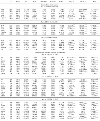
since it is already deflated and linearly detrended by construction. We subdivided the full sample into three periods: (I) 1996-2005, (II) 2006-2015, and the full sample (III) 1996-2015. Table 1 reports the descriptive statistics and some preliminary tests on all time series.

[include Table 1 about here]

2_{All calculations are exercised in MatLab R2017b. In addition, we are thankful to Kevin Sheppard for providing}

his MFE MatLab toolbox from which we used some functions including the Model Confidence Set. The toolbox is available fromhttps://www.kevinsheppard.com/MFE_Toolbox.

3_{The price series is retrieved fromhttps://www.eia.gov/dnav/pet/pet_pri_fut_s1_d.htm.} 4_{Except for WTI, all price series are retrieved from Thompson Reuters Datastream. The price series are continuous}

futures series which roll over to the nearest contract at the first day of the month (Roll method Type 0).

5_{The data is obtained fromhttp://www.policyuncertainty.com/.}

6_{We are grateful to Lutz Kilian for kindly providing the data for the global real economic activity with recent}

updates on his personal webpagehttp://www-personal.umich.edu/˜lkilian/paperlinks.html.

7_{We choose this time window, because the VIX is only available starting 1990. Choosing 1992 as a starting year}

allows us 1) have the necessaryK= 16_{quarters lag, i.e. four years, for the GARCH-MIDAS model and 2) to calculate}

We find that all time series are stationary, given the results of the Augmented Dickey-Fuller (ADF) test. Only forGREAin the first sample, the ADF test does not reject the hypothesis of a unit root in the sample. Moreover, the daily log-returns of the commodities exhibit high auto-correlation of squared returns at 12 lags (ARCH test), which suggests the use of GARCH models.

In addition to the growth rates of the macroeconomic variables, we also include the quarterly realized variance of the commodities, defined as

XRV

q =

66

X

i=1

r2

t−i,q. (11)

Moreover, we use the quarterly variance of the growth rates of the macroeconomic variablesXM V q as explanatory variable for the long-term volatility. We estimate the variance of the quarterly mac-roeconomic variables in a similar fashion as in Schwert (1989). In a first step, we filter the quarterly growth rates with a fourth-order Auto-Regressive model and four quarterly dummy variables to ac-count for seasonal effects of the growth series:

XqM =

4

X

i=1

φiXqM−i+

4

X

i=1

ηiDi+εq. (12)

In a second step, the filtered quarterly observations,εq, are squared and used as an estimator for the quarterly variance of the macroeconomic variables:

XM V

q =ε

2

q. (13)

4. Results and Discussions

We now turn to our results. We divide this section into three parts. In the first subsection, we estimate three GARCH models: the simple GARCH, the Spline-GARCH, and the GARCH-MIDAS-RV to examine whether including a time-varying long-term component can better explain the commodity volatility.

In the subsequent subsection, we estimate a total of 20 different models for each commodity, i.e. we use separately the quarterly growth rates and the quarterly variances of all explanatory mac-roeconomic and financial variables in our sample in combination with GARCH-MIDAS. Focusing on a single variable in the GARCH-MIDAS model allows us to conclude significance and direction of impact of the explanatory variables.

total of 13 models is incorporated to predict the 1-day, 1-week, and 1-month ahead volatility.

4.1. Long-term Volatility Patterns

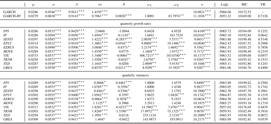
We start our analysis by examining the parameter estimations of the simple GARCH, the Spline-GARCH, and the GARCH-MIDAS-RV models with Student’s tdistribution for the period from 2 January 1996 to 31 December 2015. The estimation of these models allows to straightforwardly assess whether it is economically meaningful to decompose the commodity return volatility into high and low frequencies. Note that the GARCH-MIDAS-RV has the quarterly realized variance of each commodity return as an explanatory variable of its long-term volatility.

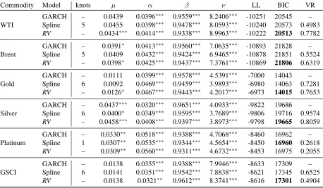
[include Table 2 about here]

The estimation results are given in Tab. 2. As expected, the GARCH-MIDAS-RVmodel, which incorporates the quarterly realized variance of commodity returns, yields the best goodness-of-fit (i.e., lowest BIC) for all commodities under consideration, except for Platinum where the Spline-GARCH is the best-suited model. In all cases, the simple Spline-GARCH model has the worst fit, given its low Log-Likelihood (LL). For the Spline-GARCH model, the knots are identified by means of the ICSS approach and the results show five structural breakpoints for WTI and Brent oil indices, six for Gold, Silver and GSCI, and only one breakpoint for Platinum.

1996 1998 2000 2002 2004 2006 2008 2010 2012 2014 2016

WTI Volatility

0 2 4 6 8 10 12

√

ht

√_τ

t(GARCH)

√_τ

t(Spline)

√_τ

t(RV)

Figure 1: Volatility (√ht) and long-term volatility (√τt) of WTI oil price returns with GARCH, Spline-GARCH, and

Tab. 2 also indicates that the short-term dynamics (i.e.αandβ) of the three models are highly significant and very similar with relatively close values. This finding thus suggests that the dif-ferences in statistical fit (LL) and goodness-of-fit (BIC) rather arise from the long-term volatility component. Engle et al. (2013) use a variance ratio to determine the explanatory value of the long-term volatility. The measure VR= V(logτt)

V_(loght) describes the proportion of variance of the logarithmic

long-term volatility and the variance of the logarithmic conditional volatility. For each GARCH-based specification, we use the estimated conditional variancebhtof the simple GARCH model as base.8 _{For the remaining models, we see that the long-term component of the Spline-GARCH and}

the GARCH-MIDAS-RVexplains the fluctuation of the variance in a range between 21% and 96%. As an illustration, we depict, in Fig. 1, the long-term components of each model for the WTI crude oil volatility. The long-term volatility pattern provided by the GARCH-MIDAS-RVfollows closely the conditional volatility dynamics.

4.2. Drivers of Long-term Volatility

We now turn to present and discuss the results from the GARCH-MIDAS regressions over the three different sample periods for each commodity, whereby the long-term volatility component is modeled as a function of each of the financial and macroeconomic variables.

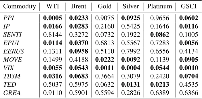
Before we present the regression analysis, we further test the legitimacy of a time-varying long-term component by means of a recently proposed regression-based misspecification test. To test the null hypothesis of a constant long-term component (simple GARCH), Conrad & Schienle (2018) suggest to run the following linear regression model:

logRVq =a0+a1Xq−1+ρlogRVq−1+ξq, (14)

where RVq is the quarterly realized variance based on the daily, standardized residuals from the simple GARCH model. Xq−1 is the lagged, quarterly macroeconomic variable. The idea behind

the test is that the realized variance should not be predictable. Hence, ifa1is statistically different

from zero, we can reject the null hypothesis of a constant long-term component. Our results show, that for all five commodities at least two variables are able to predict the realized variance. Thus, some variables might not be appropriate to predict RV, but it appears the simple GARCH model with constant long-term component is not correctly specified.9

Since a time-varying long-term component seems reasonable, we procede with the GARCH-MIDAS insample regression. This analysis allows us to identify the drivers of shocks or swings in the long-term volatility component. Without loss of generality, we solely concentrate on the

8

Note that the simple GARCH has an VR of zero. Since its long-term component is constant over time, the variance of the constant logarithmic long-term component is zero.

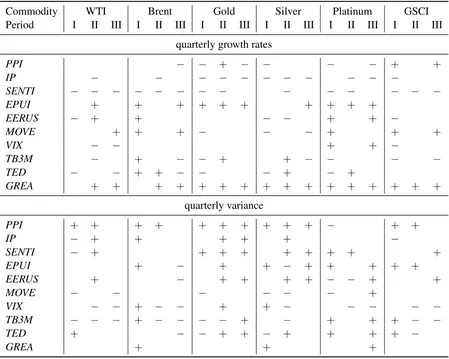
interpretation of the MIDAS parametersθ, ω1, andω2. The results are given in Tab. 3, where we

summarize the sign of the statistically significant parameterθ.10

[include Table 3 about here]

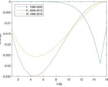
The results for the WTI crude oil indicate that the quarterly growth rates of all macroeconomic variables have significant effects on the WTI long-term volatility in at least one out of the three peri-ods we consider, exceptPPIandTB3M. In particular, the consumer sentiment (SENTI) consistently has a negative and significant impact in all three periods. Hence, when consumer sentiment rises the oil price volatility tends to decrease, which may suggest that the economy is in its stable state. As expected, the economic policy uncertainty (EPUI), the effective exchange rate for the United States (EERUS), and the global real economic activity (GREA) drive up the long-term oil price volatility. The effect of the quarterly variance of the growth rates of macroeconomic variables is however not exactly similar as thePPIandTB3Mvariables have now significant impacts. Also, the impact of the variance of the SENTI variable on long-term oil price volatility over the full period is positive. A close look at theSENTIvariable shows that for the full period, we estimate the para-meters θb= ₋0.2359, _cω1 = 1.7843, and cω2 = 2.8450. Hence, for a 1% increase ofSENTI one

quarter before, the long-term WTI volatility decreases byexp (₋0.2359_·0.0549)₋1 = ₋0.0129 or -1.29%. The highest impact is due to changes in the consumer sentiment five quarters before, i.e. a 1% increase in consumer sentiment decreases the long-term volatility in five quarters by exp (₋0.2359_·0.1094)₋1 = ₋0.0258 or₋2.58%. Figure 2 shows the full lag structure for all three sample periods and how it changed from the first to the second decade of the whole sample. In the second sample period, the impact ofSENTIis even bigger than for the full sample. As to the variance of the 3-month treasury bill rate, it negatively influences the long-term WTI volatility for all three sample periods. Thus, the U.S. oil price volatility decreases due to interest rate variability. This finding complements the observations of Barsky & Kilian (2002), who document that oil price increases (decreases) were preceded by low (high) interest rates.

The European Brent oil volatility shows similar patterns like its U.S. counterpart. Especially for the second period and the full sample, we observe that the GREAlevel is positively associated with the long-term oil price volatility. Hence, positive values in the global real economic activity index lead to higher oil price fluctuations. Kilian (2009) builds the index based on dry bulk ship cargo rates. These rates increase in times of high economic activity due to the fact that high demand meets an relatively inelastic supply curve. Thus, a positive index points towards a demand shock and an increased trading volume of commodities in general, which leads to their higher volatility. Analogously, if the GREA has a negative index, the markets cool down given the lower demand,

10

2 4 6 8 10 12 14 16

Lag

-0.035 -0.03 -0.025 -0.02 -0.015 -0.01 -0.005 0

Change

I: 1996-2005 II: 2006-2015 III: 1996-2015

Figure 2: Change of the conditional variance of WTI due to the impact of consumer sentiment (SENTI) for quarterly lags up toK= 16_.

and oil prices stabilize (less volatility). We find the GREA to be significant for all commodities in the second sub-sample. Figure 3 shows the effects of the laggedGREAlevels on the long-term volatility of the two oil indices and the three metals. While the long-term volatility of the WTI and Brent is influenced by the GREAindex from its first lag onwards, the metal volatility only reacts five quarters after and their highest reaction is observed at the seventh lag. Interestingly, we find that Brent reacts one quarter quicker to demand shocks than WTI, which could be explained by the fact that the Brent oil price is used as the benchmark for two-thirds of the world’s oil trades.

2 4 6 8 10 12 14 16 Lag

0 0.002 0.004 0.006 0.008 0.01 0.012

Change

WTI Brent Gold Silver Platinum

Figure 3: Change of the long-term conditional volatility of WTI, Brent, Gold, Silver, and Platinum due to the impact of global real economic activity (GREA) index for quarterly lags up toK= 16_{. The period spans from 2006-2015.}

(2017), which show the importance of EPUI for Gold and WTI, respectively.

4.3. Forecasting Commodity Volatility

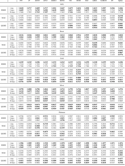
Whether the GARCH-MIDAS specifications with financial and macroeconomic variables are helpful for forecasting commodity volatility is of great interest to investors and portfolio managers. This subsection compares their predictive ability with the one of the simple GARCH, the Spline-GARCH, and the GARCH-MIDAS-RVmodels.11 _{We choose an out-of-sample period of four years}

from 3 January 2012 to 30 December 2015 (i.e.M = 1005observations), with an expanding train-ing window starttrain-ing from 2 January 1996. Three loss functions are used to compare the forecasttrain-ing performance of the different models and model specifications. They are described as follows:

RMSE= 1

M

v u u tXM

i=1

ˆ

hi−(ri−µˆi)2

,

MAE= 1

M

M X

i=1

|ˆhi−(ri−µˆi)2|,

QLIKE= 1

M

M X

i=1

log ˆhi+

(ri−µˆi)2 ˆ

hi !

,

whereˆhi is the forecasted conditional variance and the squared residual(ri−µˆi)2 is the proxy for the actual variance at timeiin the out-of-sample seti= 1, . . . , M.

Moreover, following Hansen et al. (2011), we employ the Model Confidence Set (MCS) with 10% level of significance to identify the best forecasting models and to avoid the problem of data snooping.

[include Table 4 about here]

The results of the variance forecast are given in Tab. 4. For oil price returns (WTI and Brent), the Spline-GARCH yields the best variance prediction performance and is present in the MCS of almost all loss functions over all horizons. All GARCH-MIDAS models with macroeconomic and financial variables have relatively equal performance in forecasting the oil price volatility with respect to the RMSE criterion over 1- or 5-days ahead. For the other loss functions, only the GARCH-MIDAS-GREAmodel joins the Spline-GARCH in the MCS, while the GARCH-MIDAS-VIXmodel for the Brent oil is also included in the MCS with respect to the QLIKE. Putting together with the findings in subsection 4.2, the GREA is not only suitable for explaining the in-sample volatility, but also a promising candidate to conduct forecasts of long-term oil price volatility.

11_{Due to the fact that we do not find consistent patterns for the variance of these variables, we use the growth rates}

The results for Gold show that all competing models belong to the set of equally well-performing models at the 1-day ahead forecast horizon with respect to the RMSE and at the 5- and 20-days ahead forecast horizon with respect to QLIKE. Only the GARCH-MIDAS-TB3Mmodel is present in all MCS regardless of time horizons and loss functions. This is a little bit surprising in our study, because (a) it is not significant in all in-sample estimations and (b) the direction of effects is not consistent. Its predictive power seems to suggest that it contains information about the long-term volatility which is used as a tendency for the short-term forecasts. For instance, a rising tendency in the TB3M could signal stock market booms and thus more stable Gold prices in the long-run because Gold will be less used in hedging and diversification strategies.

For Silver, the RMSE and QLIKE loss functions indicate that almost all GARCH-MIDAS mod-els with financial and macroeconomic variables, the GARCH, and the GARCH-MIDAS-RV have equal performance at the three forecasting horizons under consideration. The MAE, on the other hand, only identifies four out of 13 models with superior performance. The inclusion of SENTI, EPUI, and MOVE variables into the GARCH-MIDAS models results in lower MAE for 5- and 20-days than the other specifications. Having realized volatility as explanatory variable for the long-term volatility shows better performance for 1- and 5-days ahead forecasts.

The long-term volatility of Platinum appears to be harder to predict. We find the same mac-roeconomic variables as for Silver to be included in the MCS. While the GARCH-MIDAS-SENTI and GARCH-MIDAS-MOVE models (also simple GARCH) show good performance for 5- and 20-days horizons, the GARCH-MIDAS-EPUI and GARCH-MIDAS-RV belong to the MCS for 1-day ahead prediction.

The variance of the commodity index GSCI is relatively well predicted by all explanatory vari-ables. Only the MAE indicates that the Spline-GARCH maybe favourable.

The results from the variance forecasting show that no single GARCH-MIDAS specification is able to predict the volatility better than the others, and this result holds across all commodities. Especially, the use of theTEDto predict commodity volatility is not recommended. From 54 tests (three horizons, three loss functions, and six commodities), it is only included in 15 MCS. On the contrary, the GARCH-MIDAS model using theGREAlevel appears to have 29 inclusions.

number to the theoretical coverage, e.g. for a 95% VaR the theoretical coverage is 5%. Based on the GARCH models, we estimate the VaR as follows:

d

VaRt,p = ˆµt+ q

ˆ

htF₁−₋1p(ˆν), (15)

where F−1

1−p(ν) is the (1− p)-quantile function of the Student-t distribution with ν degrees of

freedom.12

[include Table 5 about here]

2012 2013 2014 2015 2016

-10 -5 0 5 10

WTI returns 99% VaR 97.5% VaR 95% VaR

Figure 4: Value-at-Risk forecast for WTI 2012-2015 with GARCH-MIDAS-SENTI.

The results of the VaR backtest in Table 5 can be summarized as follows. First, for the WTI and Brent crude oil as well as for GSCI, almost all models pass the VaR test from a long trading

12

position, but fail when the short trading perspective is evaluated. For the GSCI, the result may partly be explained due to the fact that a large share of the index includes crude oil. Second, the test rejects more models on the long trading positions for Gold and Silver. Finally, except for some models at 5-days ahead VaR forecast for long trading positions, all forecasting models for Platinum fail to obtain satisfactory results. Figure 4 demonstrates the VaR forecast for WTI with GARCH-MIDAS-SENTI, which has the least rejections over all VaR tests conducted (17 out of 36). On the short trading positions, i.e. traders being susceptible to earn positive returns, the GARCH-MIDAS model with the sentiment index as an explanatory variable is rejected by the backtest due to the fact that the predictions are too conservative. For example, the 95% VaR forecast which is supposed to have a coverage of 5% only yields 2.69% (27 exceptions). The 97.5% VaR only has 0.90% (9 exceptions) and the 99% VaR only has a coverage of 0.02% (2 exceptions), where 2.5% and 1% are required, respectively.13 Since the model fails to provide a sufficient estimate of the VaR at any quantile, it is rejected by the P´erignon & Smith (2008) test. Models that yield too conservative VaR estimates are costly in terms of capital requirements of banks or VaR-limits of traders. However, as mentioned above, the VaR estimates for the long trading position pass the test. Here, the coverage of the 95% VaR is 5.57% (56 exceptions).

In order to check for robustness of our in-sample and out-of-sample results, we check for sev-eral different settings of our models. First, we change the number of lags K, i.e. how many past quarters information of macroeconomic variables are used. Second, we use logarithmic differences of the macroeconomic variables instead of growth rates. Third, we attempt to incorporate the first principal component of all macroeconomic and financial variables. Fourth, instead of using the Student-tdistribution for the innovationszt, we evaluated our results assuming a Normal distribu-tion. Finally, we change the frequency of our explanatory variable, which we use at a quarterly rate, to monthly growth rates to explain the long-term volatility of daily commodity returns. For all mentioned robustness checks, the results remain qualitatively intact.

5. Conclusion

The motivation of this paper was to identify the potential drivers of the long-term volatility of commodity prices through the GARCH-MIDAS class model, at both modeling and forecasting levels. We conduct our empirical investigation in three steps including the in-sample estimation, the identification of the long-term commodity volatility drivers, and the out-of-sample volatility forecasting. In the first step, we show that disentangling long-term and short-term volatility of

13_{The exceptions can be counted by the dots in Fig. 4. For the 95% VaR the sum of all yellow, green, and red dots}

commodity futures leads to a better in-sample fit by means of the Spline-GARCH and the GARCH-MIDAS models with commodity’s realized volatility.

In the second step, we employ the GARCH-MIDAS framework to examine whether each of the financial and macroeconomic variables in our study matters for the long-term commodity volatility. We find that the long-term commodity volatility is negatively influenced by the growth rates of the consumer sentiment and the industrial production, but positively by the growth rate of the economic policy uncertainty and the level of the general real economic activity. We also investigate whether the variance of these financial and macroeconomic variables inhibits any information for the long-term commodity volatility, but we do not find any consistent results across commodity futures.

The last part of the paper uses the GARCH-MIDAS with financial and macroeconomic variables to forecast the volatility of commodities over the 1-, 5-, and 20-days ahead horizons. It is important to stress that the consistent results for in-sample estimations are not translated into forecasting performance. Thus, we find different best-suited models for each commodity. For example, the oil price volatility is best predicted with either Spline-GARCH or the GARCH-MIDAS-GREA. For Gold, the GARCH-MIDAS-TB3M is recommended for forecasting the volatility at the 1-, 5-, and 20-days ahead forecasts. For Silver and Platinum5-, we find the GARCH-MIDAS-SENTI5-, the GARCH-MIDAS-EPUI, the GARCH-MIDAS-MOVE, and the GARCH-MIDAS-RV to have equally well results. At the same time, our forecasting results show, from a risk management perspective, that the inclusion of financial and macroeconomic variables in the volatility models does not lead to better Value-at-Risk predictions than the simple GARCH model.

References

Acerbi, C., & Szekely, B. (2014). Backtesting Expected Shortfall. Risk Magazine, (pp. 76–81).

Adams, Z., & Gl¨uck, T. (2015). Financialization in commodity markets: A passing trend or the new normal? Journal of Banking & Finance, 60, 93–111. doi:10.1016/j.jbankfin.2015.

07.008.

Arouri, M. E. H., Jouini, J., & Nguyen, D. K. (2011). Volatility spillovers between oil prices and stock sector returns: Implications for portfolio management. Journal of International Money and Finance,30, 1387–1405. doi:10.1016/j.jimonfin.2011.07.008.

Asgharian, H., Hou, A. J., & Javed, F. (2013). The importance of the macroeconomic variables in forecasting stock return variance: A GARCH-MIDAS approach. Journal of Forecasting,32, 600–612. doi:10.1002/for.2256.

Bahloul, W., & Bouri, A. (2016). The impact of investor sentiment on returns and conditional volatility in U.S. futures markets. Journal of Multinational Financial Management,36, 89–102.

doi:10.1016/j.mulfin.2016.07.003.

Barsky, R., & Kilian, L. (2002). Do We Really Know that Oil Caused the Great Stagflation? A Monetary Alternative. In B. S. Bernake, & K. S. Rogoff (Eds.),NBER Macroeconomics Annual 2001(pp. 137–183). volume 16.

Basel Committee on Banking Supervision (2016). Minimum capital requirements for market risk. Technical Report January 2016. URL:www.bis.org/bcbs/publ/d352.pdf.

Batten, J. A., Ciner, C., & Lucey, B. M. (2010). The macroeconomic determinants of volatility in precious metals markets.Resources Policy,35, 65–71. doi:10.1016/j.resourpol.2009.

12.002.

Baumeister, C., Gu´erin, P., & Kilian, L. (2014). Do high-frequency financial data help forecast oil prices? The MIDAS touch at work. International Journal of Forecasting, 31, 238–252.

doi:10.1016/j.ijforecast.2014.06.005.

Baur, D. G., & Lucey, B. M. (2010). Is Gold a Hedge or a Safe Haven? An Analysis of Stocks, Bonds and Gold. Financial Review, 45, 217–229. doi:10.1111/j.1540-6288.2010.

00244.x.

Bekiros, S., Nguyen, D. K., Sandoval Junior, L., & Uddin, G. S. (2017). Information diffu-sion, cluster formation and entropy-based network dynamics in equity and commodity markets. European Journal of Operational Research, 256, 945–961. doi:10.1016/j.ejor.2016.

06.052.

Bodie, Z., & Rosansky, V. I. (1980). Risk and Return in Commodity Futures. Financial Analysts Journal,36, 27–39. doi:10.2469/faj.v36.n3.27.

Bollerslev, T. (1986). Generalized autoregressive conditional heteroskedasticity. Journal of Eco-nometrics,31, 307–327. doi:10.1016/0304-4076(86)90063-1.

B¨uy¨uks¸ahin, B., & Robe, M. A. (2011). Does ’Paper Oil’ Matter? Energy Markets’ Financializa-tion and Equity-Commodity Co-Movements. URL:http://www.ssrn.com/abstract=

1855264.

B¨uy¨uks¸ahin, B., & Robe, M. A. (2014). Speculators, commodities and cross-market linkages. Journal of International Money and Finance,42, 38–70. doi:10.1016/j.jimonfin.2013.

08.004.

Conrad, C., & Loch, K. (2015). Anticipating Long-Term Stock Market Volatility. Journal of Applied Econometrics,30, 1090–1114. doi:10.1002/jae.2404.

Conrad, C., Loch, K., & Rittler, D. (2014). On the macroeconomic determinants of long-term volatilities and correlations in U.S. stock and crude oil markets. Journal of Empirical Finance, 29, 26–40. doi:10.1016/j.jempfin.2014.03.009.

Conrad, C., & Schienle, M. (2018). Testing for an Omitted Multiplicative Long-Term Component in GARCH Models. Journal of Business & Economic Statistics, 0015, 1–14. doi:10.1080/

07350015.2018.1482759.

Daskalaki, C., Kostakis, A., & Skiadopoulos, G. (2014). Are there common factors in individual commodity futures returns? Journal of Banking and Finance,40, 346–363. doi:10.1016/j.

jbankfin.2013.11.034.

Daskalaki, C., & Skiadopoulos, G. (2011). Should investors include commodities in their portfolios after all? New evidence. Journal of Banking and Finance, 35, 2606–2626. doi:10.1016/j.

jbankfin.2011.02.022.

D¨onmez, A., & Magrini, E. (2013). Agricultural Commodity Price Volatility and Its Macroeco-nomic Determinants. Technical Report EUR 26183 EN Joint Research Centre Luxembourg.

doi:10.2791/23669.

Dwyer, A., Gardner, G., & Williams, T. (2011). Global Commodity Markets – Price Volatility and Financialisation. Bulletin, (pp. 49–58).

Ederington, L. H., & Guan, W. (2010). Longer-term time-series volatility forecasts. Journal of Financial and Quantitative Analysis,45, 1055–1076. doi:10.1017/S0022109010000372.

Engle, R. F. (1982). Autoregressive Conditional Heteroscedasticity with Estimates of the Variance of United Kingdom Inflation. Econometrica,50, 987–1007. doi:10.2307/1912773.

Engle, R. F., Ghysels, E., & Sohn, B. (2013). Stock Market Volatility and Macroeconomic Funda-mentals. Review of Economics and Statistics,95, 776–797.

Engle, R. F., & Lee, G. (1999). A long-run and short-run component model of stock return volatil-ity. In R. Engle, & H. White (Eds.),Cointegration, Causality, and Forecasting: A Festschrift in Honour of Clive W.J. Granger(pp. 475–497). Oxford: Oxford University Press.

Engle, R. F., & Rangel, J. G. (2008). The spline-GARCH model for low-frequency volatility and its global macroeconomic causes. Review of Financial Studies,21, 1187–1222. doi:10.1093/

rfs/hhn004.

Fang, L., Chen, B., Yu, H., & Qian, Y. (2018). The importance of global economic policy un-certainty in predicting gold futures market volatility: A GARCH-MIDAS approach. Journal of Futures Markets,38, 413–422. doi:10.1002/fut.21897.

Filis, G., Degiannakis, S., & Floros, C. (2011). Dynamic correlation between stock market and oil prices: The case of oil-importing and oil-exporting countries. International Review of Financial Analysis,20, 152–164. doi:10.1016/j.irfa.2011.02.014.

Ghysels, E., Santa-Clara, P., & Valkanov, R. (2004). The MIDAS Touch: Mixed Data Sampling Regression Models. CIRANO Working Papers,20, 1–33.

Ghysels, E., Sinko, A., & Valkanov, R. (2007). MIDAS Regressions: Further Results and New Directions. Econometric Reviews,26, 53–90. doi:10.1080/07474930600972467.

Hansen, P. R., Lunde, A., & Nason, J. M. (2011). The Model Confidence Set. Econometrica,79, 453–497. doi:10.3982/ECTA5771.

Karali, B., & Power, G. J. (2013). Short- and long-run determinants of commodity price volatility. American Journal of Agricultural Economics,95, 724–738. doi:10.1093/ajae/aas122.

Karali, B., & Ramirez, O. A. (2014). Macro determinants of volatility and volatility spillover in energy markets. Energy Economics,46, 413–421. doi:10.1016/j.eneco.2014.06.004.

Kilian, L. (2009). Not All Oil Price Shocks Are Alike: Disentangling Demand and Supply Shocks in the Crude Oil Market. American Economic Review, 99, 1053–1069. doi:10.1257/aer.

99.3.1053.

Kilian, L., & Vega, C. (2011). Do Energy Prices Respond to U.S. Macroeconomic News? A Test of the Hypothesis of Predetermined Energy Prices. Review of Economics and Statistics, 93, 660–671. doi:10.1162/REST{\_}a{\_}00086.

Klein, T. (2017). Dynamic Correlation of Precious Metals and Flight-to-Quality in Developed Markets. Finance Research Letters,23, 283–290. doi:10.1016/j.frl.2017.05.002.

Kupiec, P. H. (1995). Techniques for Verifying the Accuracy of Risk Measurement Models. The Journal of Derivatives,3, 73–84. doi:10.3905/jod.1995.407942.

Lintner, J. V. (1983). The potential role of managed commodity-financial futures accounts (and/or funds) in portfolios of stocks and bonds. Division of Research, Graduate School of Business

Administration, Harvard University.

Liu, Y., Han, L., & Yin, L. (2018). Does news uncertainty matter for commodity futures markets? Heterogeneity in energy and non-energy sectors. Journal of Futures Markets, 38, 1246–1261.

doi:10.1002/fut.21916.

Lucey, B. M., Sharma, S. S., & Vigne, S. A. (2017). Gold and inflation(s) – A time-varying relationship. Economic Modelling,67, 88–101. doi:10.1016/j.econmod.2016.10.008.

Narayan, P. K., Narayan, S., & Sharma, S. S. (2013). An analysis of commodity markets: What gain for investors? Journal of Banking & Finance,37, 3878–3889. doi:10.1016/j.jbankfin.

2013.07.009.

Nieto, B., Novales, A., & Rubio, G. (2015). Macroeconomic and Financial Determinants of the Volatility of Corporate Bond Returns. Quarterly Journal of Finance, 05, 1550021. doi:10.

1142/S2010139215500214.

Opschoor, A., van Dijk, D., & van der Wel, M. (2014). Predicting volatility and correlations with Financial Conditions Indexes. Journal of Empirical Finance, 29, 435–447. doi:10.1016/j.

jempfin.2014.10.003.

Pan, Z., Wang, Y., Wu, C., & Yin, L. (2017). Oil price volatility and macroeconomic fundament-als: A regime switching GARCH-MIDAS model. Journal of Empirical Finance, 43, 130–142.

doi:10.1016/j.jempfin.2017.06.005.

P´erignon, C., & Smith, D. R. (2008). A New Approach to Comparing VaR Estimation Methods. The Journal of Derivatives,16, 54–66. doi:10.3905/JOD.2008.16.2.054.

Pindyck, R. S. (2004). Volatility and commodity price dynamics. Journal of Futures Markets,24, 1029–1047. doi:10.1002/fut.20120.

Prokopczuk, M., Stancu, A., & Symeonidis, L. (2017). The economic drivers of time-varying commodity market volatility. URL:https://papers.ssrn.com/sol3/papers.cfm?

abstract_id=2678883.

Sans´o, A., Arag´o, V., & Carrion, J. (2004). Testing for changes in the unconditional variance of financial time series. Revista de Econom´ıa financiera,4, 32–53.

Schwert, G. W. (1989). Why Does Stock Market Volatility Change Over Time? The Journal of Finance,44, 1115–1153. doi:10.1111/j.1540-6261.1989.tb02647.x.

Silvennoinen, A., & Thorp, S. (2013). Financialization, crisis and commodity correlation dynamics. Journal of International Financial Markets, Institutions and Money,24, 42–65. doi:10.1016/

j.intfin.2012.11.007.

Smales, L. A. (2017). Commodity market volatility in the presence of U.S. and Chinese macroeco-nomic news. Journal of Commodity Markets,7, 15–27. doi:10.1016/j.jcomm.2017.06.

002.

Tang, K., & Xiong, W. (2012). Index Investment and the Financialization of Commodities. Finan-cial Analysts Journal,68, 54–74. doi:10.2469/faj.v68.n6.5.

Walther, T., Klein, T., Pham Thu, H., & Piontek, K. (2017). True or spurious long memory in European Non-EMU currencies. Research in International Business and Finance, 40C, 217– 230. doi:10.1016/j.ribaf.2017.01.003.

Wang, F., & Ghysels, E. (2015). Econometric Analysis of Volatility Component Models. Econo-metric Theory,31, 362–393. doi:10.1017/S0266466614000334.

Wei, Y., Liu, J., Lai, X., & Hu, Y. (2017). Which determinant is the most informative in fore-casting crude oil market volatility: Fundamental, speculation, or uncertainty? Energy Eco-nomics, 68, 141–150. URL: https://doi.org/10.1016/j.eneco.2017.09.016.

doi:10.1016/j.eneco.2017.09.016.

Yin, L. (2016). Does oil price respond to macroeconomic uncertainty? New evidence. Empirical Economics,51, 921–938. doi:10.1007/s00181-015-1027-7.

Yin, L., & Zhou, Y. (2016). What Drives Long-term Oil Market Volatility? Fundamentals versus Speculation. Economics: The Open-Access, Open-Assessment E-Journal, 10, 1–26. doi:10.

T Mean Min. Max. Stand.Dev. Skewness Kurtosis LB(12) ARCH(12) ADF

Commodities (daily returns) Jan 1st 1996-Dec 30th 2005

WTI 2501 0.0492 -12.1607 11.6594 1.9820 -0.2029 5.2754 15.7446 64.4502∗∗∗ _-49.6648∗∗∗ Brent 2610 0.0448 -14.4372 12.8982 2.2517 -0.2308 5.4517 9.7797 50.7701∗∗∗ _-52.9709∗∗∗ Gold 2610 0.0110 -5.1049 8.8872 0.8800 0.6539 12.7778 17.1831 112.6825∗∗∗ _-51.0886∗∗∗ Silver 2610 0.0205 -11.8323 7.6612 1.4473 -0.4294 8.3490 23.0132∗∗ _175.5339∗∗∗ _-51.0985∗∗∗ Platinum 2610 0.0342 -14.4173 18.6781 1.3806 1.1136 30.8952 30.6490∗∗∗ _{12.0356 -52.0306}∗∗∗ GSCI 2610 0.0350 -9.1695 6.5670 1.3058 -0.1160 4.8398 9.4775 67.5175∗∗∗ _-51.7882∗∗∗

Jan 2nd 2006-Dec 31st 2015

WTI 2514 -0.0199 -10.5782 12.1150 2.1369 -0.1592 6.2928 21.3814∗∗ _452.5556∗∗∗ _-53.5608∗∗∗ Brent 2609 -0.0176 -10.9455 12.7066 2.0985 -0.0683 6.8232 51.0998∗∗∗ _592.7609∗∗∗ _-54.3737∗∗∗ Gold 2609 0.0275 -9.8206 8.6250 1.2635 -0.3727 8.0461 27.4426∗∗∗ _130.4636∗∗∗ _-51.0980∗∗∗ Silver 2609 0.0171 -19.5185 12.3585 2.2741 -0.8740 9.2652 14.8882 141.0550∗∗∗ _-52.5413∗∗∗ Platinum 2609 -0.0033 -9.6033 16.0210 1.5176 -0.0922 11.2790 15.7196 164.1283∗∗∗ _-48.1499∗∗∗ GSCI 2609 -0.0428 -8.6486 7.2159 1.4950 -0.3046 6.3860 20.0830∗ _477.3502∗∗∗ _-53.0929∗∗∗

Jan 1st 1996-Dec 31st 2015

WTI 5015 0.0146 -12.1607 12.1150 2.0612 -0.1826 5.8927 17.6758 527.7097∗∗∗ _-73.1878∗∗∗ Brent 5219 0.0136 -14.4372 12.8982 2.1765 -0.1553 6.0644 32.4483∗∗∗ _535.3568∗∗∗ _-75.8587∗∗∗ Gold 5219 0.0193 -9.8206 8.8872 1.0887 -0.1107 10.0088 33.3773∗∗∗ _269.7001∗∗∗ _-72.2897∗∗∗ Silver 5219 0.0188 -19.5185 12.3585 1.9058 -0.8372 10.7768 17.0178 341.2088∗∗∗ _-73.7414∗∗∗ Platinum 5219 0.0154 -14.4173 18.6781 1.4507 0.4234 19.4480 19.3300∗ _84.9298∗∗∗ _-70.5618∗∗∗ GSCI 5219 -0.0039 -9.1695 7.2159 1.4040 -0.2416 5.9329 16.2624 655.5203∗∗∗ _-74.3136∗∗∗

Macroeconomic Variables (monthly growth rates) Apr 1st 1992-Oct 1st 2005

PPI 55 0.6694 -0.3376 2.0451 0.4754 0.6912 3.7751 318.2274∗∗∗ _50.1899∗∗∗ _-3.6043∗∗∗ IP 55 0.8200 -1.8292 2.8383 0.9645 -0.3809 3.1006 35.2119∗∗∗ _{14.3579 -3.2424}∗∗∗ SENTI 55 0.4590 -23.1088 21.8281 7.6340 0.0805 4.2131 41.7492∗∗∗ _32.1541∗∗∗ _-9.3907∗∗∗ EPUI 55 1.7363 -38.8710 69.5293 22.3375 0.4208 3.1595 39.2926∗∗∗ _{17.0294 -11.0963}∗∗∗ EERUS 55 0.0478 -6.9507 6.1370 3.0024 -0.2221 2.6952 21.6967∗∗ _{17.2949 -7.0971}∗∗∗ MOVE 55 1.3843 -29.3532 63.6364 18.5001 1.0442 4.1247 21.9241∗∗ _{9.1196 -10.0174}∗∗∗ VIX 55 2.3680 -40.3663 107.7626 28.2879 1.5510 5.8957 35.4489∗∗∗ _{11.1852 -10.2729}∗∗∗ TB3M 55 1.0094 -38.4615 41.4894 14.5236 0.1139 4.0666 87.7110∗∗∗ _33.2890∗∗∗ _-3.5105∗∗∗ TED 55 6.2467 -60.2941 86.1111 34.0892 0.4774 2.6466 31.6456∗∗∗ _33.4887∗∗∗ _-8.9898∗∗∗ GREA 55 -0.4675 -31.9724 50.0013 20.8700 0.8223 3.0898 164.7693∗∗∗ _48.2137∗∗∗ _-1.4067

Apr 1st 2002-Oct 1st 2015

PPI 55 0.5419 -2.5072 2.3931 0.9436 -0.5981 4.1356 40.2087∗∗∗ _{15.1128 -5.9474}∗∗∗ IP 55 0.2587 -6.3991 2.2055 1.4753 -2.5494 11.3393 45.8746∗∗∗ _32.7200∗∗∗ _-3.2404∗∗∗ SENTI 55 0.3614 -23.1088 23.3553 9.2580 0.1338 3.3880 33.7638∗∗∗ _{5.9681 -10.0613}∗∗∗ EPUI 55 2.6112 -45.3283 81.8613 25.4964 1.0549 4.3691 18.0936 11.2170 -9.1542∗∗∗ EERUS 55 -0.2340 -7.9567 7.5602 3.5305 0.1185 2.6679 34.7111∗∗∗ _{17.9774 -5.5318}∗∗∗ MOVE 55 0.8816 -38.2632 74.1710 20.6668 1.4848 5.8719 8.3091 11.6003 -8.3127∗∗∗ VIX 55 4.4193 -45.5307 160.0484 34.2312 2.1021 9.7139 30.7492∗∗∗ _{8.4924 -8.8370}∗∗∗ TB3M 55 0.8119 -80.5970 166.6667 43.9323 1.7308 8.3431 12.7389 18.4377 -6.4236∗∗∗ TED 55 10.6581 -63.4146 246.1538 52.2457 2.2308 10.1778 18.6416∗ _{13.1449 -8.8564}∗∗∗ GREA 55 14.6714 -52.8075 64.3385 30.4095 -0.3424 2.1175 155.1052∗∗∗ _49.8877∗∗∗ _-2.1508∗∗

Apr 1st 1992-Oct 1st 2015

PPI 95 0.5767 -2.5072 2.3931 0.7532 -0.7862 6.0136 70.8559∗∗∗ _28.7945∗∗∗ _-6.8992∗∗∗ IP 95 0.5351 -6.3991 2.8383 1.3503 -2.2119 11.4121 60.7998∗∗∗ _42.0781∗∗∗ _-4.2607∗∗∗ SENTI 95 0.6426 -23.1088 23.3553 8.3201 0.2527 3.7418 38.7771∗∗∗ _{8.6220 -12.9977}∗∗∗ EPUI 95 2.7076 -45.3283 81.8613 24.7079 0.8304 3.8843 25.0137∗∗ _{12.1545 -13.2026}∗∗∗ EERUS 95 0.1405 -7.9567 7.5602 3.2155 -0.0054 2.7492 23.7173∗∗ _{15.9138 -8.0968}∗∗∗ MOVE 95 1.8373 -38.2632 74.1710 20.5543 1.1986 4.7469 14.3955 9.1704 -12.0629∗∗∗ VIX 95 4.2099 -45.5307 160.0484 32.1412 1.9710 8.8980 36.8007∗∗∗ _{8.0812 -12.6911}∗∗∗ TB3M 95 -0.0771 -80.5970 166.6667 34.1781 2.1582 13.2354 18.4462 30.7764∗∗∗ _-8.4102∗∗∗ TED 95 7.8327 -63.4146 246.1538 45.9179 2.0660 10.5898 28.4977∗∗∗ _19.9667∗ _-11.7807∗∗∗ GREA 95 4.8672 -52.8075 64.3385 26.9702 0.3593 2.3448 309.0392∗∗∗ _81.8343∗∗∗ _-2.8191∗∗∗

Table 1: Descriptive statistics of commodity returns and growth rates of macroeconomic variables.

Note: Rejection of the respective hypothesis at 1%, 5% and 10% is marked by∗∗∗_,∗∗_{, and}∗_{, respectively. LB(12) and}

Commodity Model knots µ α β ν LL BIC VR

WTI

GARCH – 0.0439 0.0396∗∗∗ _0.9559∗∗∗ _8.2406∗∗∗ _{-10251 20545 –}

Spline 5 0.0455 0.0398∗∗∗ _0.9478∗∗∗ _8.0593∗∗∗ _{-10240 20573 0.4983}

RV – 0.0434∗∗∗ _0.0414∗∗∗ _0.9338∗∗∗ _8.9963∗∗∗ _{-10222 20513 0.7782}

Brent

GARCH – 0.0391∗ _0.0413∗∗∗ _0.9560∗∗∗ _7.0635∗∗∗ _{-10893 21828 –}

Spline 5 0.0409 0.0432∗∗∗ _0.9424∗∗∗ _6.9465∗∗∗ _{-10878 21851 0.5524}

RV – 0.0398∗ _0.0425∗∗∗ _0.9437∗∗∗ _7.3761∗∗∗ _{-10869 21806 0.6319}

Gold

GARCH – 0.0111 0.0399∗∗∗ _0.9578∗∗∗ _4.5391∗∗∗ _{-7000 14043 –}

Spline 6 0.0092 0.0469∗∗∗ _0.9459∗∗∗ _3.9893∗∗∗ _{-6980 14063 0.7281}

RV – 0.0126∗ _0.0467∗∗∗ _0.9443∗∗∗ _4.2017∗∗∗ _{-6973 14015 0.7653}

Silver

GARCH – 0.0437∗∗∗ _0.0320∗∗∗ _0.9651∗∗∗ _4.0933∗∗∗ _{-9822 19686 –}

Spline 6 0.0400∗ _0.0349∗∗∗ _0.9595∗∗∗ _3.7689∗∗∗ _{-9806 19716 0.9574}

RV – 0.0458∗∗∗ _0.0408∗∗∗ _0.9397∗∗∗ _3.8973∗∗∗ _{-9798 19665 0.8059}

Platinum

GARCH – 0.0330∗∗ _0.0518∗∗∗ _0.9388∗∗∗ _4.7068∗∗∗ _{-8460 16962 –}

Spline 1 0.0307∗∗ _0.0535∗∗∗ _0.9344∗∗∗ _4.5654∗∗∗ _{-8450 16960 0.2618}

RV – 0.0309∗∗ _0.0560∗∗∗ _0.9311∗∗∗ _4.6732∗∗∗ _{-8453 16975 0.2055}

GSCI

GARCH – 0.0138 0.0355∗∗∗ _0.9388∗∗∗ _7.9946∗∗∗ _{-8633 17309 –}

Spline 6 0.0141 0.0351∗∗∗ _0.9542∗∗∗ _7.8838∗∗∗ _{-8621 17345 0.6525}

RV – 0.0138 0.0321∗∗ _0.9612∗∗∗ _8.3741∗∗∗ _{-8616 17301 0.4904}

Table 2: Parameter estimation results of the GARCH, Spline-GARCH, and GARCH-MIDAS-RV: 2 January 1996 - 31 December 2015.

Note: The asterisks∗∗∗_,∗∗_{, and}∗_{indicate significance at 1%, 5%, and 10%, respectively. LL is the Log-Likelihood and}

Commodity WTI Brent Gold Silver Platinum GSCI

Period I II III I II III I II III I II III I II III I II III

quarterly growth rates

PPI _{− −} + _{− − − −} + +

IP _{− − − − − − − − − − −}

SENTI _{− − − − − − − − − − − − − −}

EPUI + + + + + + + + + +

EERUS ₋ + + _{− −} + + ₋

MOVE + + + _{− − −} + + +

VIX _{− −} + + ₋

TB3M ₋ + _{− −} + + _{− − − −}

TED _{− −} + + _{− − −} + ₋ +

GREA + + + + + + + + + + + + + + + +

quarterly variance

PPI + + + + + + + + + + ₋ + +

IP ₋ + + + + + ₋

SENTI ₋ + + + + + + + + +

EPUI + ₋ + + ₋ + + + + +

EERUS + ₋ + + + + _{− −} + +

MOVE _{− − − − − −} +

VIX _{− −} + _{− −} + + _{− − − − −}

TB3M _{− − −} + _{− − − −} + ₋ + + + _{− −}

TED + _{− −} + + ₋ + + + + ₋

GREA + + +

Table 3: Regression results for GARCH-MIDAS model using macroeconomic and financial variables.

PPI IP SENTI EPUI EERUS MOVE VIX TB3M TED GREA GARCH RV Spline

WTI

RMSE

1-day 3.4620 3.4717 3.4609 3.4717 3.4561 3.4647 3.4679 3.4636 3.4588 3.4633 3.4587 3.4366 3.4466 5-days 3.6689 3.6779 3.6705 3.6582 3.6638 3.6692 3.6651 3.6967 3.6679 3.6604 3.6661 3.7518 3.6738 20-days 3.7608 3.7893 3.7525 3.7457 3.7605 3.7603 3.7426 3.8008 3.7671 3.7372 3.7550 3.9878 3.7846

MAE

1-day 0.7105 0.7173 0.6833 0.7054 0.7044 0.7090 0.7011 0.7157 0.7190 0.6906 0.7067 0.7220 0.6738 5-days 0.7670 0.7844 0.7410 0.7554 0.7631 0.7680 0.7546 0.7789 0.7789 0.7420 0.7628 0.8526 0.7293 20-days 0.8466 0.8864 0.8217 0.8271 0.8489 0.8539 0.8251 0.8629 0.8673 0.8093 0.8405 1.0394 0.7966

QLIKE

1-day 0.8807 0.8864 0.8304 0.8725 0.8753 0.8763 0.8637 0.8938 0.8943 0.8457 0.8745 0.9077 0.8461 5-days 0.9300 0.9475 0.8830 0.9165 0.9267 0.9294 0.9090 0.9465 0.9470 0.8894 0.9229 1.0410 0.8985 20-days 1.0081 1.0532 0.9651 0.9838 1.0099 1.0159 0.9793 1.0258 1.0353 0.9554 0.9988 1.2578 0.9600

Brent

RMSE

1-day 3.0136 3.0106 3.0028 3.0022 3.0052 3.0112 3.0068 2.9924 2.9959 3.0038 3.0008 2.9952 3.0020 5-days 3.2042 3.2030 3.1999 3.1934 3.1989 3.2002 3.2020 3.2011 3.1962 3.1834 3.1963 3.2741 3.2395 20-days 3.3086 3.3167 3.3050 3.2908 3.3114 3.3040 3.3033 3.3126 3.3044 3.2665 3.3017 3.5075 3.4219

MAE

1-day 0.6585 0.6670 0.6525 0.6620 0.6656 0.6656 0.6631 0.6599 0.6667 0.6430 0.6606 0.6830 0.6461 5-days 0.7072 0.7198 0.7036 0.7109 0.7182 0.7167 0.7150 0.7158 0.7210 0.6866 0.7115 0.7837 0.7043 20-days 0.7733 0.7960 0.7759 0.7751 0.7936 0.7852 0.7845 0.7886 0.7927 0.7442 0.7812 0.9387 0.7830

QLIKE

1-day 0.8238 0.8408 0.8134 0.8335 0.8417 0.8392 0.8340 0.8415 0.8484 0.8007 0.8330 0.8747 0.8492 5-days 0.8637 0.8842 0.8558 0.8721 0.8851 0.8795 0.8760 0.8865 0.8914 0.8362 0.8739 0.9720 0.9067 20-days 0.9217 0.9535 0.9200 0.9272 0.9534 0.9406 0.9386 0.9494 0.9578 0.8862 0.9356 1.1416 0.9776

Gold

RMSE

1-day 1.6349 1.6345 1.6286 1.6315 1.6332 1.6363 1.6335 1.6324 1.6350 1.6340 1.6359 1.6154 1.6206 5-days 1.7210 1.7189 1.7202 1.7187 1.7180 1.7207 1.7162 1.7149 1.7219 1.7183 1.7192 1.7351 1.7229 20-days 1.7288 1.7304 1.7294 1.7274 1.7252 1.7284 1.7219 1.7236 1.7300 1.7271 1.7266 1.7618 1.7384

MAE

1-day 0.2628 0.2593 0.2557 0.2566 0.2560 0.2597 0.2568 0.2519 0.2559 0.2576 0.2590 0.2640 0.2617 5-days 0.2775 0.2743 0.2702 0.2716 0.2693 0.2737 0.2701 0.2654 0.2712 0.2717 0.2725 0.2889 0.2837 20-days 0.2902 0.2907 0.2824 0.2851 0.2810 0.2850 0.2816 0.2769 0.2829 0.2840 0.2834 0.3249 0.3110

QLIKE

1-day 0.4122 0.4108 0.4093 0.4098 0.4087 0.4127 0.4061 0.4060 0.4105 0.4111 0.4113 0.4143 0.4079 5-days 0.4667 0.4639 0.4625 0.4628 0.4629 0.4680 0.4584 0.4598 0.4650 0.4661 0.4652 0.4719 0.4611 20-days 0.4756 0.4787 0.4745 0.4712 0.4694 0.4759 0.4612 0.4727 0.4760 0.4767 0.4744 0.4948 0.4754

Silver

RMSE

1-day 3.4798 3.4808 3.4786 3.4844 3.4695 3.4722 3.4790 3.4746 3.4827 3.4593 3.4787 3.4671 3.4754 5-days 3.6118 3.6079 3.5963 3.6027 3.6112 3.6053 3.6117 3.6080 3.6355 3.5970 3.6056 3.6028 3.6394 20-days 3.6370 3.6847 3.6231 3.6284 3.6349 3.6294 3.6414 3.6361 3.6705 3.6447 3.6312 3.6480 3.7435

MAE

1-day 0.7748 0.7733 0.7640 0.7675 0.7710 0.7672 0.7721 0.7704 0.7822 0.7656 0.7724 0.7571 0.8025 5-days 0.8113 0.8145 0.7972 0.8008 0.8134 0.8022 0.8091 0.8064 0.8205 0.8117 0.8068 0.7988 0.8636 20-days 0.8472 0.8769 0.8324 0.8327 0.8544 0.8369 0.8449 0.8437 0.8618 0.8800 0.8413 0.8531 0.9605

QLIKE

1-day 0.8651 0.8624 0.8474 0.8546 0.8627 0.8543 0.8629 0.8610 0.8812 0.8547 0.8615 0.8418 0.9129 5-days 0.9121 0.9178 0.8902 0.8987 0.9137 0.9027 0.9086 0.9074 0.9290 0.9135 0.9071 0.8942 0.9852 20-days 0.9499 0.9984 0.9299 0.9340 0.9569 0.9387 0.9469 0.9463 0.9720 0.9970 0.9461 0.9597 1.1089

Platinum

RMSE

1-day 0.9786 0.9725 0.9751 0.9532 0.9836 0.9814 0.9907 0.9811 0.9838 0.9798 0.9822 0.9505 0.9954 5-days 1.0680 1.0511 1.0461 1.0604 1.0520 1.0451 1.0671 1.0523 1.0509 1.0484 1.0457 1.0609 1.0931 20-days 1.1481 1.0992 1.0862 1.1429 1.0803 1.0706 1.1447 1.0889 1.0791 1.0842 1.0709 1.1617 1.2173

MAE

1-day 0.2944 0.2810 0.2740 0.2718 0.2861 0.2814 0.2906 0.2803 0.2836 0.2796 0.2816 0.2712 0.3101 5-days 0.3368 0.3162 0.3048 0.3225 0.3154 0.3078 0.3273 0.3112 0.3115 0.3094 0.3084 0.3285 0.3582 20-days 0.3976 0.3603 0.3394 0.3846 0.3482 0.3359 0.3828 0.3441 0.3412 0.3440 0.3373 0.4025 0.4368

QLIKE

1-day 0.4903 0.4751 0.4683 0.4679 0.4791 0.4760 0.4876 0.4753 0.4776 0.4760 0.4754 0.4663 0.5087 5-days 0.5327 0.5110 0.5013 0.5192 0.5098 0.5043 0.5264 0.5075 0.5070 0.5081 0.5038 0.5237 0.5564 20-days 0.6020 0.5583 0.5389 0.5906 0.5428 0.5317 0.5878 0.5422 0.5359 0.5433 0.5317 0.6092 0.6466

GSCI

RMSE

1-day 1.1906 1.1889 1.1854 1.1918 1.1892 1.1878 1.1857 1.1867 1.1898 1.1863 1.1877 1.1871 1.1876 5-days 1.2466 1.2481 1.2458 1.2478 1.2469 1.2466 1.2453 1.2512 1.2483 1.2430 1.2467 1.2619 1.2520 20-days 1.2660 1.2749 1.2673 1.2655 1.2714 1.2640 1.2635 1.2725 1.2680 1.2606 1.2652 1.3184 1.2765

MAE

1-day 0.2536 0.2578 0.2499 0.2565 0.2558 0.2560 0.2569 0.2592 0.2575 0.2505 0.2558 0.2593 0.2412 5-days 0.2695 0.2774 0.2680 0.2717 0.2742 0.2726 0.2741 0.2779 0.2737 0.2677 0.2724 0.2929 0.2606 20-days 0.2926 0.3085 0.2974 0.2932 0.3031 0.2958 0.2976 0.3025 0.2965 0.2951 0.2953 0.3513 0.2841

QLIKE

1-day 0.4201 0.4253 0.4158 0.4263 0.4215 0.4250 0.4242 0.4288 0.4260 0.4148 0.4240 0.4249 0.4277 5-days 0.4452 0.4525 0.4423 0.4508 0.4480 0.4504 0.4492 0.4562 0.4509 0.4398 0.4492 0.4634 0.4602 20-days 0.4601 0.4754 0.4602 0.4647 0.4684 0.4650 0.4643 0.4729 0.4659 0.4553 0.4638 0.5147 0.4740

Table 4: Out-of-sample forecasting results tested with loss functions.

Note: We report RMSE, MAE, and QLIKE results from out-of-sample variance forecasting with 1-day, 5-day, and 20-days ahead horizons. Bold face values indicate models which are included in the Model Confidence Set M90%with