Is GDP more volatile in developing countries after taking the shadow economy into account? Evidence from Latin America

Munich Personal RePEc Archive

Is GDP more volatile in developing

countries after taking the shadow

economy into account? Evidence from

Latin America

Solis-Garcia, Mario and Xie, Yingtong

Macalester College, University of Wisconsin-Madison

30 March 2017

Is GDP more volatile in developing countries after taking the

shadow economy into account? Evidence from Latin America

Mario Solis-Garcia†

Macalester College

Yingtong Xie‡

University of Wisconsin-Madison

March 30, 2017

Abstract

Why is GDP more volatile in developing countries? In this paper we propose an explanation that can account for the substantial differences in the volatility of measured real GDP per capita between de-veloping and developed countries. Our explanation involves the often overlooked fact that dede-veloping economies have a sizable shadow economy. We build a two-sector model that distinguishes between measured (formal) and total (formal and shadow) outputs; using data from Latin America, our model results suggest that developing and developed economies are fairly similar in terms of the volatility of total real GDP. We also document an apparent puzzle, in that the model suggests that the volatility of the size of the shadow economy should be substantially larger than what is observed in the real world. We believe that this may be indicative of frictions that prevent agents from optimally moving between the formal and shadow economies.

JEL codes: E26, E32, O17.

Keywords: shadow economy, business cycles, DSGE models, Bayesian estimation.

∗_{We thank Michael Alexeev, Ceyhun Elgin, Pete Ferderer, Gary Krueger, Karine Moe, and Jesús Rodríguez-López for valuable}

comments on earlier versions of the paper, as well as seminar participants at the 2013 and 2014 Latin American and Caribbean Economic Association meetings, 2014 Southern Economic Association meetings, and 2014 Missouri Valley Economic Association meetings. We also thank Julia Blount for excellent editorial assistance. We gratefully acknowledge support from the Allianz Life Insurance Company Student Summer Research Fund.

† _{Corresponding author. Department of Economics, Macalester College, 1600 Grand Avenue, St. Paul, MN 55105. E-mail:}

1

Introduction

There is a sizable difference in the volatility ofmeasuredreal GDP per capita (hereafter, RGDP) between

developing and developed countries. In particular, the volatility of measured RGDP in Latin American

countries is significantly higher than that in the United States and Canada, as shown inFigure 1:

0 5 10 15 20 25

USA CAN COL HND MEX URY GTM CRI DOM AVG BOL BRA CHL ECU PAN VEN ARG PRY JAM PER TTO

R

G

D

P

vo

la

ti

lit

y

(p

e

rce

n

t)

Figure 1: Measured RGDP volatility, selected countries, 1950-2011.

Notes: Measured RGDP volatility is calculated as the standard deviation of the residual of a regression of the logarithm of the variable against a linear and a quadratic time trends. The data for the regression runs from 1950 to 2011, except for Chile, Dominican Republic, and Paraguay (data starts in 1951) and Jamaica (1953). “AVG” denotes the average standard deviation across all countries. SeeAppendix Afor a list of the country codes.

The average volatility of measured RGDP for the developing countries in the figure is 2.6 times as large

as that in the United States. In particular, Colombia and Honduras are 1.5 and 1.7 times as volatile, while

the corresponding values for Peru and Trinidad and Tobago are 4.3 and 6.1, respectively.

Several studies have tried to account for this empirical fact. For example,Neumeyer and Perri(2005)

restrictions.Aguiar and Gopinath(2007) focus instead on the contribution of stochastic trends in developing

economies, which add to the overall volatility of their business cycle.

In this paper we provide a different perspective, based on the often overlooked fact that the size of the

shadow economy is larger in developing countries than it is in developed ones. Since the economic activity

of the shadow sector is at best poorly measured and, consequently, is not included in the values shown

inFigure 1, we claim that the actual volatility of RGDP in developing economies (or more precisely, in

economies with a sizable shadow economy) is not as large as shown in the figure. In other words, this paper

argues that there is a connection between the high values of measured RGDP volatility and the presence of

a large shadow sector.

For our purposes, the shadow economy is the sum of all market-based production of (legal) goods and

services that are not reported to government authorities (we exclude illegal and home production; seeSection

2for a detailed account). These firms choose to remain underground for a variety of reasons; arguably, the

most important is to avoid payment of taxes or social security contributions, labor market regulations, or

compliance with administrative procedures.

Conventional wisdom places firms in the shadow economy as an “escape valve” from the effects of

recessions: the output of these productive units (relative to measured output) tends to increase in bad times

and decrease in good times. A contribution of this paper is to investigate the relationship between the shadow

economy—and its escape valve role—and the volatility of measured RGDP in developing economies.

Using data from a set of Latin American and Caribbean countries (we add the United States and Canada

as well),1_{we find that the volatility of total RGDP is about 1.3%, substantially lower than the corresponding}

value for measured RGDP (5.5%). The main assumption that we require is that measured RGDP only

includes the activities of the formal sector. (This key assumption is also used byFernández and Meza 2015

1_{We analyze countries in Latin America and the Caribbean since the size of the shadow economy is relatively large in these}

in their study of the Mexican shadow employment.)

We envision the following mechanism: in less developed countries, measured RGDP fluctuations are

amplified as negative shocks to total factor productivity (TFP) in the formal sector generate a movement

of productive factors from the formal to the shadow sector,2 hence lowering measured RGDP whiletotal

RGDP (which includes both formal andunmeasured shadow production) is not lowered significantly. This

implies that total RGDP volatility should be smaller than measured RGDP volatility as the latter fails to

consider the behavior of a large portion of economic activity.

In order to test our mechanism and assess the connection between measured RGDP volatility and the

shadow sector, we build a two-sector dynamic stochastic general equilibrium (DSGE) model that includes

formal (measured) and shadow (unmeasured) activities. In our model, a representative consumer/producer

has access to a formal technology that employs both capital and labor but can also work with a shadow

technology that requires only labor input. Both the formal and shadow technologies are subject to TFP

shocks. The simulated data from our model generates a value of total RGDP volatility that is twice as

large (2.6%) but fairly homogeneous among countries, irrespective of the development status of the country

(using simulated data, measured RGDP volatility equals 9.6%, almost double the real-world value). These

results suggest that countries have a similar level of volatility once we take into account the dynamics of the

shadow economy.

Our model can also successfully reproduce two correlations found in the real world, namely, (1) a

negative relationship between the size of the shadow economy and measured RGDP, and (2) a positive

correlation between the volatility of the size of the shadow economy and the volatility of measured RGDP.

However, our model fails to generate the low volatility of the size of the shadow sector that is observed in

the data. We believe that this may be indicative of frictions that prevent agents from optimally switching

between the production technologies.

2_{We do not model this particular mechanism but offer some potential causes for it: lack of unemployment benefits—particularly}

1.1 Connection with the literature

The use of DSGE models to understand the behavior of the shadow economy is fairly recent;3_{several papers}

stand out in the literature and here we discuss their connection to our work. Ihrig and Moe(2004) use the

data fromSchneider and Enste(2000) to document three empirical relations for a cross-section of countries

in 1990. First, a negative and convex relationship between the size of the shadow economy and a country’s

measured RGDP; second, a positive relationship between the size of the shadow economy and tax rates, and

third, a negative relationship between the size of the shadow economy and (tax) enforcement. They build

a two-sector model—which is the basis of the model used in this paper—and calibrate it to the economy

of Sri Lanka. Their simulations verify that the model is broadly consistent with their empirical findings.

While our emphasis is not on the connection between tax rates and enforcement and the size of the shadow

economy, we are able to confirm their first empirical finding using more recent data (Schneider, Buehn,

and Montenegro 2010). Moreover, we improve upon their modeling strategy by adding a leisure choice to

the consumer/producer so that switching between sectors is not an “either-or” option. Finally, we take the

model to the data for a variety of countries and we use both calibration and Bayesian estimation procedures

to derive our results.

Using a two-sector DSGE model,Busato and Chiarini(2004) conclude that adding a shadow economy

to the model generates three main findings: first, a better fit to Italian data (relative to the indivisible labor

model of Hansen 1985); second, a stronger propagation mechanism of TFP shocks, and third, a greater

degree of risk sharing due to the presence of two different labor alternatives. To calibrate the model, they

use the formal/shadow output decomposition ofBovi(1999) and they calibrate the share of shadow labor

using the values found inSchneider and Enste(2000). Other parameters are set to match some target values

of the Italian economy. Relative to their work, we go one step ahead both in the scope (many Latin American

3_{The following papers share a DSGE approach to the shadow economy but do not center their analysis on its relation to business}

economies as opposed to Italy) and in the parametrization of the model (by adding a Bayesian estimation

component). We decide not to incorporate the particular functional form for the utility function, which is

based onCho and Cooley(1994).

Finally, we need to mention the contributions of Conesa, Díaz-Moreno, and Galdón-Sánchez (2001,

2002) andRestrepo-Echavarría(2014) as their work is closest to ours. First consider the work ofConesa

et al. Their goal is to account for the differences in volatility of output between countries by using a model

that includes a shadow economy. That said, their mechanism is based on the relationship between the

wage premium (defined as the wage difference between working in the formal and shadow sectors) and

the participation rate. Other things the same, a lower wage premium reduces the participation rate, since

the opportunity cost of working in the shadow sector goes down. In turn, shocks to the productivity of the

registered firms will shift a larger proportion of agents between both sectors. Hence, countries with different

values for the wage premium will experience different fluctuations in response to TFP shocks.4 _{At a deeper}

level, their results rely on the shadow economy as an external production alternative but do not use shadow

economy size estimates to derive the main results.5 _{In contrast, our model does not make any assumptions}

about the connection between the wage premium and the participation rate; as mentioned above, we use the

estimates fromSchneider et al.(2010) as our starting point and then build our model from the bottom up

while taking these values into account.

The work ofRestrepo-Echavarríashares our interest in determining the effects of the shadow economy

over the business cycle but is considerably different to what we do below. She looks at how the relative

volatility of consumption to GDP is affected by the presence of a shadow economy and quantifies this

4 _{Their mechanism assumes a link between the participation rate and the shadow economy, in that a low participation rate}

suggests a high activity in the shadow sector. Schneider and Enste(2000) discuss this mechanism as the basis of a measurement approach (seeSection 3) and characterize it as a weak indicator of the size of the shadow economy for two reasons. First, a low participation rate may have other causes different from an active shadow economy and second, people may opt to work in the formal and shadow economy at the same time. We choose to remain agnostic about the role of the participation rate and focus on the direct effect of TFP shocks instead.

5 _{For example, inConesa et al. (2002) the authors use a simulated grid of participation rates and then use these values as}

in a two-sector DSGE model with formal and shadow consumption goods; she finds that including the

shadow economy can better account for the relative volatility of consumption. As shown below, our model

is interested in the volatility of GDP on its own; in addition, while we keep a two-sector model in the

background we don’t distinguish between different consumption goods. Overall, we believe that her work

and ours are analyzing different implications of the shadow economy.

1.2 Roadmap

The rest of the paper is structured as follows. A brief discussion of the measurement issues of the shadow

economy are presented inSection 2. The empirical facts that motivate the paper are found inSection 3while

Section 4 presents a dynamic model of the shadow sector. Section 5 discusses the parametrization of our

model and our results are presented inSection 6. Section 7concludes.

2

Characterizing and measuring the shadow economy

The literature on the shadow economy shows that the terminology can sometimes be loosely interchanged

for other concepts that are not necessarily equivalent. The Organisation for Economic Co-operation and

Development (seeOECD 2002) has defined thenon-observed economyas a term that stands in for the

fol-lowing categories of production: (1) underground production (goods and services that are kept off the market

in order to avoid taxes or regulations), (2) illegal production (goods and services that are prohibited by law),

(3) informal sector production (goods and services that are produced by firms that are either unregistered

or below a threshold of employment), (4) production of households for own-final use (goods and services

produced within the household for self-consumption), and (5) statistical underground (goods and services

that should be accounted for but are not because they are overlooked by statistical agencies).

Our notion of the shadow economy consists of the sum of underground (1) and informal sector (3)

state that illegal production is left out. In addition, the statistical underground is hard to quantify, and

production of households for own-final use—often called home production—considers a different set of

productive activities that are not meant to be traded in the market.6₎

Measuring the size of the shadow economy is far from an easy task.Schneider and Enste(2000) discuss

three main methodologies to calculate this value; here we discuss them briefly and refer the reader to their

paper for additional details. By “direct approaches,”Schneider and Ensterefer to direct surveys and samples

that attempt to quantify the number of productive entities that belong in the shadow economy. However, by

their very nature, these methods are prone to providing biased estimates as respondents may be inclined to

lie about their formal/shadow status. Moreover, the cost of implementing methods of this kind makes it

unlikely to be used in a frequent basis.

The second methodology relies on macroeconomic indicators to infer the size of the shadow economy

over time. Schneider and Enstedenote this broad methodology as “indirect approaches” and list five

tech-niques. First, we can look at thediscrepancy between the expenditure and income measures in national

ac-counts: since these (by construction) need to be the same, any difference between expenditures and income

values of GDP could provide a measure of the shadow economy. Similarly, we can look at thediscrepancy

between the official and actual labor force: a fall in the participation rate could point to an active shadow

economy. In thetransactions approach, the researcher conjectures a stable relation between the total volume

of transactions and GDP and uses this as a base to quantify the size of the shadow economy. Thecurrency

demand approachassumes that all shadow economy transactions are carried out in cash, so that an increase

in shadow economy activity will result in an increase in the demand for currency. Finally, thephysical

input methoduses the (near unit) elasticity between electricity and GDP as well as the growth of electricity

consumption to infer the growth of the shadow economy.

The third methodology (known as the “model approach”) uses structural econometric models to back out

the size of the shadow economy. In a nutshell, the main idea behind this class of models is that the shadow

economy does not have a single cause and does not exhibit a single effect when it operates over time.

Hence, a structural econometric framework can be used to infer the size of the shadow sector by looking

(simultaneously) both at the hypothesized causes of the shadow economy (e.g., tax rates and regulation) as

well as the hypothesized effects (e.g., participation rates and currency demand). This methodology is often

called the multiple-indicators multiple-causes model (MIMIC) and is the technique used bySchneider et al.

(2010) to derive the values that we use in this study.7

3

Some empirical facts

In what follows, we first compare the the standard deviation of measured RGDP (as shown inFigure 1) with

that of total RGDP as implied by the presence of a shadow sector. For each country/year pair, we set total

RGDP to equal measured RGDP times 1+YS/F, whereYS/F denotes the shadow economy size (relative to

measured RGDP; in what follows we use the estimates ofSchneider et al. 2010).

We first show that the standard deviation of measured RGDP is larger that of total RGDP. We then

document a negative relationship between measured RGDP and the size of the shadow economy as well as

a positive correlation between the volatility of measured RGDP and the volatility of the size of the shadow

economy. While we’re not the first to document the negative relationship between RGDP and shadow sector

size, to the best of our knowledge we are the first to document the positive correlation between the volatilities

of these variables. (SeeAppendix Afor the data sources, the list of countries included in the analysis, as

well as for a detailed explanation regarding variable construction for each of the figures below.)

7_{We are aware of the work ofElgin and Öztunalı(2012), who build longer time series of the size of the shadow economy (60}

3.1 Measured and total RGDP volatility

We first verify that for our sample of countries, total RGDP volatility is smaller than measured RGDP

volatility. Although the values we use are restricted to the period 1999-2007 (which corresponds to the

range of estimates in the work ofSchneider et al.), this result can be clearly seen in Figure 2 below (the

diagonal represents the 45◦_line).

0 2 4 6 8 10 12 14 16 18

0 2 4 6 8 10 12 14 16 18

ARG

BRA CHL _COL

DOM

ECU

JAM MEX

PAN _PER PRY

TTO URY

USA

VEN

RGDP volatility (total)

RGDP volatility (measured)

Figure 2: Measured and total RGDP volatility.

Measured RGDP volatility averages 5.5% while total RGDP volatility averages 1.3% (the value for

measured RGDP volatility does not correspond to the one shown inFigure 1since the periods involved in

the calculations are different). An interesting feature ofFigure 2is that for the United States and Canada

(see the marker nearest to the United States), measured and total RGDP volatility are nearly identical—a

direct consequence of the small size of their shadow economies. Moreover, a larger shadow sector does

not necessarily imply that total volatility is lower: for example, Venezuela’s shadow sector averages 33.8%

3.2 Measured RGDP and shadow economy size

We now show that measured RGDP and the size of the shadow economy are negatively correlated. To help

visualize the relationship, we use the average ratio of measured RGDP in a particular country relative to

measured RGDP in the United States.

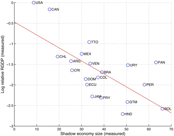
Figure 3 plots the logarithm of this variable together with the size of the shadow economy for the

countries in our sample (we add the best-fitting trendline as well). The correlation coefficient between both

series is -0.68; the main message derived fromFigure 3is that, on average, countries with a higher measured

RGDP tend to have smaller shadow economies.

0 10 20 30 40 50 60 70

−3

−2.5

−2

−1.5

−1

−0.5

0

ARG

BOL BRA

CAN

CHL

COL CRI

DOM ECU

GTM

HND JAM

MEX

PAN

PER

PRY TTO

URY USA

VEN

Shadow economy size (measured)

Log relative RGDP (measured)

Figure 3: Log (relative) measured RGDP and size of the shadow economy.

We also calculate the percent deviations from trend for measured RGDP and the size of the shadow

economy over time after using a linear-quadratic detrending procedure. We find that the shadow economy is

a countercyclical variable: the percent deviations from trend for that variable are negatively correlated with

Country Correlation Country Correlation

Argentina -0.99 Honduras -0.88

Bolivia -0.71 Jamaica -0.98

Brazil -0.89 Mexico -0.97

Canada -0.84 Panama -0.24

Chile -0.81 Paraguay -0.79

Colombia -0.55 Peru -0.65

Costa Rica -0.31 Trinidad and Tobago -0.78

Dominican Republic -0.93 United States -0.91

Ecuador -0.83 Uruguay -0.94

Guatemala -0.79 Venezuela -0.99

Average -0.79

Table 1: Correlation coefficient, percent deviation from trend in {RGDP, shadow economy}.

3.3 Measured RGDP and shadow economy volatilities

The last empirical finding that we document is the positive correlation between the volatilities of measured

RGDP and the size of the shadow economy.Figure 4shows a scatterplot for these two variables. The figure

suggests that, on average, countries that exhibit a high volatility in measured RGDP also exhibit a high

volatility in the size of the shadow economy (the correlation coefficient between both series is 0.34).

0 0.1 0.2 0.3 0.4 0.5 0.6 0.7 0.8 0.9 1

0 2 4 6 8 10 12 14 16 18 ARG BOL BRA CHL COL CRI DOM ECU GTM HND JAM MEX PAN PER PRY TTO URY USA VEN

Shadow economy size volatility (measured)

RGDP volatility (measured)

4

Model

We first present the model and then characterize its equilibrium in detail. Our model followsIhrig and Moe

(2004) with some modifications. The economy has a representative consumer/producer who has access to

a primary technology that produces output using capital and labor according to a Cobb-Douglas production

function (associated with the formal sector) but can also work with a second technology that operates in the

shadow sector and only requires labor input. Both formal and shadow technologies are subject to

productiv-ity shocks. There is a government that levies taxes on formal sector output and uses these resources to fund

a sequence of expenditure.

The consumer’s problem corresponds to choosing sequences of consumptionCt, leisure Lt, investment

Xt, formal laborNFt, and shadow laborNSt to solve

max E0

∞

∑

t=0

βt(logCt+φlogLt)

s.t. Ct+Xt= (1−τt)zFtKtαNFt1−α+BzStN_Stγ

Kt+1= (1−δ)Kt+Xt

T =Lt+NFt+NSt.

In the above,φ≥0 denotes the weight of leisure in the utility function;τt∈[0,1]stands for the formal sector

tax rate;zFt is TFP for the formal sector;Kt denotes the formal sector capital stock;α ∈(0,1)is the share

of capital in aggregate output;B>0 is a normalizing constant (which will be important in our calibration

exercise to set the right shadow/formal output ratio);zSt is TFP for the shadow sector;γ∈(0,1]is the labor

share of shadow output; andT >0 is the total amount of hours available per period.

We include a government sector to account for the potential effect that tax rates have over the size of the

of non-productive expenditureGt and that it satisfies its period-by-period budget constraint, following

Gt=τtzFtKtαNFt1−α.

4.1 Characterization of equilibrium

SettingYFt ≡zFtKtαNFt1−α,YSt ≡BzStNStγ, andYt ≡YFt+YSt, it is a simple task to show that the model’s

equilibrium is characterized by8

C_t−1 = αβEtCt−+11(1−τt+1)YF,t+1Kt−+11+β(1−δ)EtCt−+11 (4.1)

φCt = (1−α)(1−τt)YFtNFt−1Lt (4.2)

φCt = γYStN_St−1Lt (4.3)

Kt+1 = (1−δ)Kt+Xt (4.4)

T = Lt+NFt+NSt (4.5)

YFt = zFtKtαNFt1−α (4.6)

YSt = BzStNStγ (4.7)

Yt = YFt+YSt (4.8)

Yt = Ct+Xt+Gt (4.9)

Gt = τtYFt. (4.10)

Equation (4.1) is the usual intertemporal condition found in standard dynamic models. Equations (4.2)

and (4.3) represent the model’s intratemporal conditions; we have two of these as the marginal utility of

consumption should be equated with the marginal utilities of working for the formal and shadow sectors.

The rest of the equilibrium conditions are standard: equation (4.4) is the law of motion of (formal

tor) capital; (4.5) is the consumer’s time constraint; (4.6) and (4.7) are the formal and shadow production

technologies; (4.8) is our measure of total output; (4.9) is the aggregate feasibility condition; and (4.10)

represents equilibrium government spending.

We also add the laws of motion for the tax rate and formal and shadow TFP:9

τt = (1−ρτ)τ+ρττt−1+ετt

zFt = (1−ρF)zF+ρFzF,t−1+εFt

zSt = (1−ρS)zS+ρSzS,t−1+εSt.

In the above,{τ,zF,zS}denote steady-state values. In addition, for j∈ {τ,F,S},ρj∈(−1,1),E(εjt) =0,

and var(εjt) =σ2j. We also assume a potential correlation between the innovations to formal and shadow

TFP. Hence, we inferE(εFtεSt) =ϕFSσFσS.

4.2 Steady state

(In the sections that follow, variables without time subscripts denote steady state values.) We now find the

closed-form solutions for the system’s steady state values; these will be relevant to the calibration exercise

we perform inSection 5.2. We start by setting T =zF =zS=1; after some algebra, we obtain a set of

closed-form solutions. First, the formal sector’s capital stockKas a function of formal sector labor:

K=

αβ(1−τ) 1−β(1−δ)

1/(1−α)

NF ≡ωKNF. (4.11)

Second, shadow economy laborNSas a function of the normalizing constantB:

NS=

γ

(1−α)(1−τ)ω_Kα

1/(1−γ)

B1/(1−γ)≡ωSB1/(1−γ). (4.12)

Third, consumptionCas a function ofBand formal sector labor:

C= (1−α)(1−τ)ω α

K[1−ωSB1/(1−γ)−NF]

φ .

Finally, formal sector laborNF as a function ofB,φ, and other parameter values:

NF =

(1−α)(1−τ)ωα

K−[(1−α)(1−τ)ωKαωS+φ ωSγ]B1/(1−γ)

φ[(1−τ)ωα

K−δ ωK] + (1−α)(1−τ)ωKα

. (4.13)

4.3 Impulse-response analysis

Before proceeding to the parametrization, it’s useful to see how the model behaves in response to shocks to

TFP. Since we speculate that productivity shocks shift resources between sectors, we would like to see the

magnitude of these changes under reasonable parameter values.10 _{We present impulse-response functions}

for formal and total output in response to a 1% negativeinnovation to formal and shadow TFP; by doing

this, we want to compare the behavior of measured output (formal) and how it compares to total output given

the same innovation.

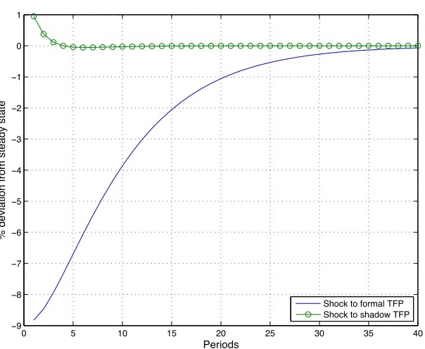
We first consider the response of formal sector output. Figure 5 shows that a negative innovation to

formal sector TFP decreases formal output by almost 9% (relative to its steady state) on impact. While

this is expected, the figure also shows the influence of a negative innovation to shadow sector TFP: shadow

output rises on impact by roughly 1% and quickly returns to the steady state.

Figure 6shows the behavior of total output as the economy receives shocks to formal and shadow TFP.

The impulse-response function shows that a negative shock to formal TFP reduces total output by nearly 5%

on impact. A negative shock to shadow TFP decreases total output a bit over half a percent point.

These results are consistent with our conjecture: a negative shock to formal-sector TFP reduces

mea-10_{For this exercise we set the discount rateβto 0.96 and the capital shareαto 0.33. All the remaining values correspond to the}

0 5 10 15 20 25 30 35 40

−9

−8

−7

−6

−5

−4

−3

−2

−1 0 1

Formal sector output

Periods

% deviation from steady state

Shock to formal TFP Shock to shadow TFP

Figure 5: Impulse-response of formal sector output.

sured RGDP by 9% yet total RGDP falls by 5% only. This suggests that the importance of shocks to formal

and shadow TFP is not trivial.

5

Parametrization

We now describe the parametrization details of our model. First, we list the data sources behind our choice

of observable variables and specify the targets between steady state values and real-world averages. We then

explain our calibration strategy, which depends on whether the country under analysis has formal labor data

available or not. Finally, we present the Bayesian priors we use in our econometric exercise.

We group the model’s parameters in the vectorΘ:

Θ={τ,zF,zS,NF,YS/F;α,β,φ,δ,B,γ,ρF,ρS,ρτ,σF,σS,στ,ϕFS},

0 5 10 15 20 25 30 35 40 −5

−4.5 −4 −3.5 −3 −2.5 −2 −1.5 −1 −0.5 0

Total output

Periods

% deviation from steady state

Shock to formal TFP Shock to shadow TFP

Figure 6: Impulse-response of total output.

5.1 Observable variables and data sources

We use five main variables as observables.11 First, we obtain measured RGDP (Y_Ftobs) and TFP (zobs_Ft ) from the Penn World Table 8.1 (Feenstra, Inklaar, and Timmer 2015); we take these series to correspond to model

variablesYFt andzFt. From the same source, we also obtain the ratio of government expenditure to GDP

(τ_tobs) that, given the period-by-period budget balance assumption, is equivalent to the model’s tax rateτt.

From the Total Economy Database (TED), we get total hours worked and create a measure of formal

labor input (Nobs

Ft ), where hours are expressed relative to 5000 hours per year. Finally, fromSchneider et al.

(2010) we obtain the value of the shadow economy (Yobs

St/Ft), expressed as a fraction of measured output; we

use this value to back out shadow sector GDP (Yobs

St ), which is the actual variable we use as an observable.

In taking the model to the data we face the following problem: a subset of countries in the TED database

do not have statistics on hours worked.12 _{This creates some issues with the estimation procedure since we}

cannot use this observable variable for all the countries in the sample. To resolve this difficulty, we design a

11_{SeeAppendix Afor additional details on the observable variables.}

12 _{These countries are Bolivia, the Dominican Republic, Guatemala, Honduras, Panama, and Paraguay. See the Technical}

joint calibration and estimation strategy that allows us to maximize the use of information that the variable

provides.

5.2 Calibration

The set of calibrated parameters is given byΘ_C≡ {τ,zF,zS,NF,YS/F;α,β,φ,B,ρF,ρτ,σF,στ}. First con-sider the steady state values{τ,zF,zS,NF,YS/F}. We setzF =zS=1 and map the remaining values to the

sample averages of the variables defined inSection 5.1: for each country, we calculate the steady state tax

rateτ, the steady state formal labor shareNF, and the steady state shadow-to-formal GDP ratioYS/F.

For the remaining elements in Θ_C, we fix the share of capital incomeα to 0.33 and the household’s discount factor β to 0.96. (These values are standard in the literature and are consistent with an annual

frequency as well.) We then obtain a long sample of values for TFP and tax rates (from 1950 to 2011, using

the same sources as detailed inAppendix A) and calculate correlation and volatility coefficients (i.e.,ρjand

σj for j∈ {τ,F}) for each series. Finally, to obtain the values forφ andB, we need to consider whether

data for formal labor is available or not. This is discussed below.

5.2.1 Formal labor data available

When formal labor data are available, our strategy follows a two-step approach. First, we calibrate parameter

Bto be consistent with the steady state valuesNF andYS/F; second, we use the value of Balong with the

steady stateNF value to calibrate parameterφ.

To obtain the calibrated value ofB, note that by construction

YS/F =

YS

YF

=ω

γ

SB1/(1−γ)

ωα

KNF

Hence, we can solve forBdirectly; we get

B=

_Y

S/FωKαNF

ω_Sγ

1−γ

. (5.2)

WithBat hand, we can solve forφfrom (4.13):

φ=(1−α)(1−τ)ω α

K[1−ωSB1/(1−γ)−NF]

NF[(1−τ)ωKα−δ ωK] +ωSγB1/(1−γ)

. (5.3)

By inspection,B andφ depend both on steady state values{τ,NF,YS/F}as well as parameters{γ,δ}

(both directly and viaωK andωS). Since the latter are estimated via Bayesian methods, we putBandφ as

direct functions ofγandδ so that they are updated at every iteration following (5.2) and (5.3).

5.2.2 No formal labor data available

When there is no available formal labor data, our approach changes slightly relative to the one described

above. We start by rewriting (4.13) as

NF =ωF1−ωF2B1/(1−γ) (5.4)

where

ωF0 ≡ φ[(1−τ)ωKα−δ ωK] + (1−α)(1−τ)ωKα

ωF1 ≡ (1−α)(1−τ)ωKα/ωF0

We combine (5.4) and (5.1) to get

YS/F=

ω_SγB1/(1−γ)

ωα

KNF

= ω

γ

SB1/(1−γ)

ω_Kα[ωF1−ωF2B1/(1−γ)]

and from this equation we can solve forB:

B=

"

YS/FωKαωF1

ω_Sγ+Y_S/Fωα

KωF2 #1−γ

. (5.5)

Equation (5.5) shows thatBdepends on steady state values{τ,Y_S/F}and parameters{γ,δ,φ}. Hence, we putBas a direct function of{γ,δ,φ}so that its value is updated at every iteration following (5.5). The

details on how we handle parameterφare discussed inSection 5.3.

5.3 Bayesian priors

For all countries, we estimate parameters in the vectorΘ_E≡ {δ,γ,ρS,σS,ϕFS}using the prior distributions

shown inTable 2. We add measurement errors on all of our observable variables, which we set to Gamma

distributions with mean and standard deviations equal to 0.125 and 0.0722 of the empirical standard

devia-tions from each observable variable.

Parameter Description Distribution Mean SD

δ Depreciation rate Beta 0.1 0.025

γ Shadow labor share Beta 0.5 0.2

ρS Autocorrelation Beta 0.5 0.2

σS Standard deviation Inverse Gamma 0.05 0.02

ϕFS Correlation Modified Beta* 0.0 0.3

* The modified Beta distribution is defined over the interval[−1,1].

Table 2: Prior distributions.

As mentioned above, a subsample of countries does not have data for formal labor. In this case, we have

average and standard deviation of the (calibrated) value ofφfor the countries that do have formal labor data.

Once this is done, we impose a Gamma prior distribution and use these values for the remaining countries.

Table 3shows the details on the prior forφ.13,14

φj, j= Mean estimate

Argentina 3.7875

Brazil 2.7318

Chile 4.0691

Colombia 3.4545

Costa Rica 2.7952

Ecuador 3.1978

Jamaica 3.1187

Mexico 3.9772

Peru 2.8556

Trinidad and Tobago 3.9768

Uruguay 2.8076

Venezuela 4.0570

Average 3.4024

Standard deviation 0.5459

Table 3: Obtaining the prior distribution forφ.

6

Results and analysis

As a first step, we use the model to generate time series for formal output and the size of the shadow

economy. We use the simulated data to verify the claim that total RGDP volatility is lower than measured

RGDP volatility given that we now consider the shadow economy’s output. We then show that the model

data are able to replicate the negative relationship between (relative) measured RGDP and the size of the

shadow economy, and the positive relationship between the volatilities of measured RGDP and the size of

the shadow economy.

13_{Since this is not a problem for the two developed countries in the sample—Canada and the United States—we take the average}

over the sample of Latin American countries that have labor data available. We have checked whether including Canada and the U.S. makes a difference in terms of our results, but it doesn’t seem that this is the case.

14_{To obtain the estimates inTable 3, we run one chain of 1 million draws, discarding the first 750 thousand draws. In all cases,}

6.1 Measured and total RGDP volatility

As mentioned in the introduction, our conjecture is that the difference in RGDP volatility between

develop-ing and developed countries can be accounted for by the mismeasurement of RGDP. To test that conjecture,

we obtain the measure of measured and total RGDP for all countries in the sample and derive a volatility

measure for both series.Figure 7replicatesFigure 2using artificial data from the model.

0 2 4 6 8 10 12 14 16 18 20

0 2 4 6 8 10 12 14 16 18 20 BRA

COL CRI

DOM ECU GTM HND JAM MEX PAN PER PRY TTO URY USA VEN

RGDP volatility (total

−

from model)

RGDP volatility (measured − from model)

Figure 7: Measured and total RGDP volatility (model data).

Visual inspection shows that for all the countries in the sample, total RGDP volatility estimates are

lower than measured RGDP volatility estimates. In particular, most values are clustered between 2 and

4%: the average value for the total RGDP volatility is 2.6% with a standard deviation of 1.0%, while the

corresponding values for measured RGDP volatility are 9.6% and 4.0%. As is the case in the real world,

6.2 Consistency checks

We now put our model through a couple of consistency checks. We verify that the simulated data are

able to replicate the empirical regularities outlined in Section 3, namely, a positive relationship between

formal RGDP and the size of the shadow economy, and a negative relationship between the volatility of

both variables.15

6.2.1 Measured RGDP and shadow economy size

Figure 8 relates formal sector relative RGDP and shadow sector size using the simulated data from the

model. Our results support a negative relationship between relative RGDP and the size of the shadow

sector; to allow for a quick comparison,Figure 9contains the same values asFigure 3.

0 10 20 30 40 50 60 70

−3 −2.5 −2 −1.5 −1 −0.5 0 ARG BOL BRA CAN CHL COL CRI DOM ECU GTM HND JAM MEX PAN PER PRY TTO URY USA VEN

Shadow economy size (measured − from model)

Log relative RGDP (measured

−

from model)

Figure 8: (Log) Relative RGDP and size of the shadow economy (model data).

By inspection, both figures are very similar, which suggests that the model does a good job at capturing

the features of the real world. (The correlation coefficient using simulated data is -0.59; real-world data

0 10 20 30 40 50 60 70

−3

−2.5

−2

−1.5

−1

−0.5

0

ARG

BOL BRA

CAN

CHL

COL CRI

DOM ECU

GTM

HND JAM

MEX

PAN

PER

PRY TTO

URY USA

VEN

Shadow economy size (measured)

Log relative RGDP (measured)

Figure 9: (Log) Relative RGDP and size of the shadow economy (real world).

(Bolivia, Dominican Republic, Guatemala, Honduras, Panama, and Paraguay) then we can see thatFigure 8

andFigure 9are nearly identical.16

6.2.2 Measured RGDP and shadow economy volatilities

We now take a look at the relationship between the volatilities of formal RGDP and the size of the shadow

economy. We follow the same logic as above and present two graphs to contrast our results.Figure 10shows

the relationship that results from model data, whileFigure 11is identical toFigure 4. We use the same scale

in both axes to facilitate comparison between graphs.

The positive relation between both variables is evident from both figures (the correlation coefficient

using model data is 0.36 while the one using real-world data is 0.34), yet there is a clear difference between

them: the volatilities of measured RGDP and shadow economy size are larger in the model than in the data,

asTable 4confirms:

0 0.5 1 1.5 2 2.5 3 3.5 4 0 2 4 6 8 10 12 14 16 18 20 ARG BOL BRA CAN COL CRI DOM ECU GTM HND JAM MEX PAN PER PRY TTO URY USA VEN

Shadow economy size volatility (measured − from model)

RGDP volatility (measured

−

from model)

Figure 10: Volatilities of RGDP and size of the shadow economy (model data).

0 0.5 1 1.5 2 2.5 3 3.5 4

0 2 4 6 8 10 12 14 16 18 20 ARG BOL BRA CHL COL CRI DOM ECU GTM JAM MEX PAN PER PRY TTO URY USA VEN

Shadow economy size volatility (measured)

RGDP volatility (measured)

Variable Observed Simulated data

Measured RGDP 5.5205 9.6285

Shadow economy size 0.3426 1.2272

Table 4: Volatility (sample average).

6.3 A volatility puzzle?

The results above suggest that our mechanism holds promise in accounting for the higher volatility of

mea-sured RGDP in Latin American countries. However, the evidence also shows a disconnection from the

theoretical predictions of the model and the real world.

From our results, theory suggests that we should observe a higher volatility both in measured RGDP

and in the size of the shadow economy. Using the values contained in Table 4, the model’s measured

RGDP volatility is 1.7 times the real-world measured RGDP volatility, yet the model’s shadow economy

size volatility is 3.6 times as high as the observed value. At face value, this result implies that agents in the

real world do not switch back and forth between the formal and shadow technologies. For some reason, the

shadow economy’s “escape valve” role does not seem to be used to its maximum.17

7

Conclusion

In this paper, we propose a mechanism to account for the substantial difference in the volatility of measured

RGDP between developing and developed countries; this mechanism involves the fairly overlooked fact that

developing economies have a sizable shadow economy. We build a model that includes a shadow economy

and distinguishes between measured (formal) and total (shadow and formal) output. The results of our model

show that economies in North and South America, including the Caribbean, are fairly similar in terms of

total RGDP volatility (2.6%, compared to 1.3% using real-world data). We document an apparent puzzle in

17_{A seminar participant suggested thinking about the shadow economy as an absorbent state: once the agent uses the shadow}

that the model suggests that the volatility of the size of the shadow economy should be substantially larger

than what is observed in the real world. We believe that this may be indicative of frictions that prevent

agents from optimally moving between production technology.

This paper adds to our understanding of the shadow economy and its relationship with business cycles

in general. Understanding the connection between these two concepts (loosely speaking, how the shadow

economy actually operates as an escape valve) should prove useful to characterize the properties of the

business cycle in developing economies. Its conclusions may also serve as a handy tool for policymakers

as oftentimes their efforts are directed at affecting the size of the shadow economy (either by attempting to

formalize producers or changing the rules of the game by altering the country’s tax policy).18

References

Mark Aguiar and Gita Gopinath. Emerging market business cycles: the cycle is the trend. Journal of

Political Economy, 115(1):69–102, 2007.

Maurizio Bovi. An improvement of the Tanzi method for the estimation of Italian underground economy.

English version of the paper: “Un miglioramento del metodo di Tanzi per la stima dell’economia

somm-ersa in Italia.” Rivista di Statistica Ufficiale dell’ISTAT, vol. 2/99, F. Angeli, Roma, 1999.

Francesco Busato and Bruno Chiarini. Market and underground activities in a two-sector dynamic

equilib-rium model. Economic Theory, 23(4):831–61, 2004.

Jang-Ok Cho and Thomas Cooley. Employment and hours over the business cycle. Journal of Economic

Dynamics and Control, 18(2):411–32, 1994.

Giuseppe Ciccarone, Francesco Giuli, and Enrico Marchetti. Search frictions and labor market dynamics in

a real business cycle model with undeclared work. Economic Theory, pages 1–34, 2015.

Pareto-Juan Carlos Conesa, Carlos Díaz-Moreno, and José Enrique Galdón-Sánchez. Underground economy and

aggregate fluctuations. Spanish Economic Review, 3(1):41–53, 2001.

Juan Carlos Conesa, Carlos Díaz-Moreno, and José Enrique Galdón-Sánchez. Explaining cross-country

di!erences in participation rates and aggregate fluctuations. Journal of Economic Dynamics and Control,

26(2):333–45, 2002.

Ceyhun Elgin and Oguz Öztunalı. Shadow economies around the world: model based estimates. Working

Paper 2012/05, Boˇgaziçi University, Department of Economics, 2012.

Robert Feenstra, Robert Inklaar, and Marcel Timmer. The next generation of the Penn World Table.

Ameri-can Economic Review, 105(10):3150–82, 2015.

Andrés Fernández and Felipe Meza. Informal employment and business cycles in emerging economies: The

case of Mexico. Review of Economic Dynamics, 18(2):381–405, 2015.

Nobert Fiess, Marco Fugazza, and William Maloney. Informal self-employment and macroeconomic

fluc-tuations. Journal of Development Economics, 91(2):211–26, 2010.

Pedro Gomis-Porqueras, Adrian Peralta-Alva, and Christopher Waller. The shadow economy as an

equilib-rium outcome. Journal of Economic Dynamics and Control, 41:1–19, 2014.

Gary Hansen. Indivisible labor and the business cycle. Journal of Monetary Economics, 16(3):309–28,

1985.

Jane Ihrig and Karine Moe. Lurking in the shadows: the informal sector and government policy. Journal of

Development Economics, 73(2):541–77, 2004.

Beth Ingram, Narayana Kocherlakota, and Eugene Savin. Using theory for measurement: an analysis of the

Pablo Neumeyer and Fabrizio Perri. Business cycles in emerging economies: the role of interest rates.

Journal of Monetary Economics, 52(2):345–80, 2005.

OECD. Measuring the non-observed economy: a handbook. Organization for Economic Co-operation and

Development, Paris, 2002.

Paulina Restrepo-Echavarría. Macroeconomic volatility: the role of the informal economy. European

Economic Review, 70:454–69, 2014.

Friedrich Schneider and Dominik Enste. Shadow economies: Size, causes, and consequences. Journal of

Economic Literature, 38(1):77–114, 2000.

Friedrich Schneider, Andreas Buehn, and Claudio Montenegro. Shadow economies all over the world: new

estimates for 162 countries from 1999 to 2007. Policy Research Working Paper 5356, World Bank, 2010.

Mario Solis-Garcia and Yingtong Xie. Technical appendix: Are business cycles more volatile in developing

countries after taking the shadow economy into account? Evidence from Latin America. Unpublished

manuscript, 2016.

A

Data appendix

A.1 Country list

The analysis includes Argentina (ARG), Bolivia (BOL), Brazil (BRA), Canada (CAN), Chile (CHL),

Colom-bia (COL), Costa Rica (CRI), the Dominican Republic (DOM), Ecuador (ECU), Guatemala (GTM),

Hon-duras (HND), Jamaica (JAM), Mexico (MEX), Panama (PAN), Paraguay (PRY), Peru (PER), Trinidad and

A.2 Section 3 details

Data sources We obtain (measured) RGDP from the Penn World Table 8.1 (Feenstra et al. 2015,

calcu-lated as the ratio of seriesrgdpnaandpop) and shadow economy size (relative to measured RGDP) from

Schneider et al.(2010).

Figure 2 We calculate total RGDP as follows: for each countryiin the sample and for eacht∈ {1999,2007},

define

RGDPTOT_i,t =RGDPi,t×

1+Y_iS_,t/F

whereY_iS_,t/F denotes the shadow economy size (relative to measured RGDP) for countryiin yeart. We then transform measured and total RGDP levels into percent deviations from trend. Given that several of the

countries under consideration have experienced recurrent crises, a linear trend may not be the best choice to

detrend the data; hence, we allow for a quadratic term along the usual linear trend. In this sense, we run the

following regressions for each country in our sample:

log(RGDPi,t) = β0,i+β1,it+β2,it2+εi,t

log(RGDPTOT_i,t ) = β_0,TOTi +β1,TOTi t+β2,TOTi t2+εiTOT,t ,

where the residualsεi,t andε_iTOT_,t are our measure of detrended RGDP, on which we calculate the standard

deviation to obtain the values shown in the graph.

Figure 3 We calculate relative RGDP (with respect to the United States) as follows: for each countryiin

the sample and for eacht∈ {1999, . . . ,2007}, we define the variable

RELGDPi,t=

RGDPi,t

RGDPUSA,t

so that RELGDPi,t denotes the RGDP ratio between countryiand the United States in yeart. Once this

variable is calculated, we derive the measure of relative RGDP by taking the simple average over the sample

ofT periods available:

RELGDPi=

1 9

2007

∑

t=1999

RELGDPi,t.

The variable that is plotted in the figure is the logarithm of the value above. Finally, the shadow economy

size is the simple average of the values obtained fromSchneider et al.(2010).

Figure 4 We transform (measured) RGDP and shadow economy size levels into percent deviations from

trend following the same guidelines as in Figure 2, though we make some small changes to the way we

calculate RGDP volatility in this case. For each countryiin the sample and for eacht∈ {1950, . . . ,2011},

we run the following regression:

log(RGDPi,t) =γ0,i+γ1,it+γ2,it2+ηi,t, (A.1)

where the residualsηi,t are our measure of detrended RGDP, on which we calculate the standard deviation

to obtain the values shown in the graph. Since the size of the shadow economy is expressed as a percentage

relative to measured RGDP, we do not need to log the dependent variable as in equation (A.1). Hence, we

run the following regression for each countryiin our sample and eacht∈ {1999,2007}:

Y_iS_,t/F =θ0,i+θ1,it+θ2,it2+µi,t. (A.2)

A.3 Section 5 details

Data sources We obtain TFP (series rtfpna) and the share of government expenditure (series csh_g)

from the Penn World Table 8.1 (Feenstra et al. 2015). We take formal hours from the series “Total hours

worked” from The Conference BoardTotal Economy DatabaseTM_{, May 2016,}

http://www.conference-board.org/data/economydatabase/. Data sources on RGDP and the size of the shadow economy are

detailed inSection A.2.

Observable variables We use percent deviations from trend as observable variables. Measured and

shadow RGDP, formal TFP, and formal hours are detrended following (A.1); tax rates follow (A.2).

B

Parameter appendix

B.1 Steady state values

We map the steady state values in our model to the sample averages of the variables defined inSection 5.1.

The values for the steady state triple{τ,NF,YS/F}are shown below.

B.2 Calibration (first stage)

The set of calibrated parameters is given byΘ_C≡ {α,β,φ,B,ρF,ρτ,σF,στ}. We setα=0.33 andβ=0.96 for all countries. The values for {ρF,ρτ,σF,στ}are derived from sample averages for each country and presented inTable 6below.

As mentioned inSection 5.2, parameters{B,φ}are determined at the same time as the Bayesian

Country τ NF YS/F

Argentina 0.1008 0.1412 0.2530

Bolivia 0.1751 N/A 0.6607

Brazil 0.1510 0.1640 0.3904

Canada 0.1387 0.1620 0.1571

Chile 0.1802 0.1414 0.1928

Colombia 0.0988 0.1396 0.3733

Costa Rica 0.1451 0.1806 0.2574

Dominican Republic 0.1254 N/A 0.3186

Ecuador 0.2064 0.1490 0.3240

Guatemala 0.1334 N/A 0.5047

Honduras 0.133 N/A 0.4832

Jamaica 0.1816 0.1502 0.3477

Mexico 0.0926 0.1329 0.3001

Panama 0.1816 N/A 0.6314

Paraguay 0.1258 N/A 0.3867

Peru 0.1683 0.1350 0.5804

Trinidad and Tobago 0.1174 0.1273 0.3340

United States 0.1233 0.1608 0.0863

Uruguay 0.1619 0.1455 0.5064

Venezuela 0.2432 0.1198 0.3384

Average 0.1492 0.1464 0.3713

N/A: no data available for formal hours.

Country ρF ρτ σF στ

Argentina 0.9246 0.7586 0.0430 0.0140

Bolivia 0.9055 0.8007 0.0408 0.0128

Brazil 0.9753 0.9317 0.0327 0.0190

Canada 0.7691 0.8304 0.0178 0.0063

Chile 0.8718 0.8621 0.0477 0.0122

Colombia 0.8336 0.8470 0.0212 0.0056

Costa Rica 0.9263 0.9558 0.0261 0.0068

Dominican Republic 0.8310 0.8083 0.0426 0.0146

Ecuador 0.8922 0.8774 0.0366 0.0146

Guatemala 0.9769 0.8210 0.0192 0.0063

Honduras 0.7491 0.9076 0.0367 0.0110

Jamaica 0.8755 0.8659 0.0330 0.0210

Mexico 0.9184 0.8676 0.0294 0.0052

Panama 0.6282 0.8919 0.0356 0.0148

Paraguay 0.8433 0.7804 0.0367 0.0104

Peru 0.9540 0.6920 0.0479 0.0118

Trinidad and Tobago 0.9063 0.9292 0.0428 0.0131

United States 0.8385 0.6778 0.0141 0.0060

Uruguay 0.8132 0.8292 0.0366 0.0105

Venezuela 0.8926 0.7859 0.0457 0.0249

Average 0.8663 0.8360 0.0343 0.0120

Table 6: Calibrated values (first stage).

B.3 Estimation and calibration (second stage)

The set of estimated parameters is given byΘ_E≡ {δ,γ,ρS,σS,ϕFS}; the priors for each parameter are listed

inTable 2. We now present the mean estimates for these parameters, as well as the implied values for the

pair{B,φ}.19,20

19_{Recall that for the set of countries without formal labor data, parameterBis backed out from steady state and estimated values,}

Country Estimated Calibrated

δ γ ρS σS ϕFS B φ

Argentina 0.0900 0.2708 0.4007 0.0314 0.3726 0.1632 3.7875

Bolivia 0.1037 0.1824 0.4578 0.0287 -0.0108 0.1971 3.3290

Brazil 0.1071 0.1661 0.4845 0.0278 0.0966 0.1694 2.7318

Canada 0.1245 0.1749 0.5025 0.0276 0.1927 0.0776 3.6720

Chile 0.1213 0.1776 0.5098 0.0283 0.1133 0.0811 4.0691

Colombia 0.1129 0.1850 0.5043 0.0278 0.1170 0.1546 3.4545

Costa Rica 0.1047 0.2089 0.5054 0.0282 0.0806 0.1505 2.7952

Dominican Republic 0.1083 0.1917 0.5070 0.0307 0.3750 0.1466 3.3031

Ecuador 0.1044 0.1898 0.4888 0.0283 0.2051 0.1391 3.1978

Guatemala 0.1037 0.1804 0.4729 0.0276 0.1175 0.1814 3.3375

Honduras 0.1073 0.1806 0.5032 0.0276 0.1789 0.1770 3.3037

Jamaica 0.1031 0.1884 0.4640 0.0276 -0.1417 0.1514 3.1187

Mexico 0.1201 0.1610 0.5288 0.0279 0.3201 0.1514 3.9772

Panama 0.1060 0.1885 0.4422 0.0291 0.1132 0.1949 3.2909

Paraguay 0.1060 0.1904 0.4803 0.0284 0.0469 0.1633 3.3209

Peru 0.1080 0.1786 0.4827 0.0279 0.1417 0.2040 2.8556

Trinidad and Tobago 0.1157 0.2015 0.5389 0.0309 0.1991 0.1351 3.9768

United States 0.0981 0.1850 0.4645 0.0275 0.0403 0.0543 4.0129

Uruguay 0.1132 0.1788 0.5274 0.0288 0.2899 0.1918 2.8076

Venezuela 0.1364 0.1729 0.7228 0.0356 0.5920 0.1004 4.0570

Average 0.1097 0.1877 0.4994 0.0289 0.1720 0.1492 3.4199

* No formal labor data are available for this country.