Munich Personal RePEc Archive
Optimal Equilibrium State in Two-Sector
Growth Model
Yashin, Pete
UPEC, LKMZ
1 February 2017
Online at
https://mpra.ub.uni-muenchen.de/76524/
Optimal Equilibrium State in Two-Sector Growth Model
Pete Yashin
UPEC, LKMZ
Lozovaya Town, 24 Svobody St., Kharkiv Province (Ukraine) yashin.p.v@mail.ru
Abstract
The paper studies a two-sector growth model for two cases: with flexible technology and with fixed coefficients. Different states of economic equilibrium (steady states) are compared. We find that the price of investment goods with respect to the price of consumer goods should be changed if the equilibrium state has shifted. Therefore, the aggregate production function cannot be considered as a purely technical. We assume that the income distribution is determined by the direct proportionality between the profits and the investment. Then the resulting function of aggregate output is continuous and differentiable in the domain of definition, even if the technology is fixed. In the last case the function has diminishing returns of capital under Uzawa capital-intensity condition; the state of economic equilibrium is stable only when this condition is valid. We suggest that the optimal is an equilibrium state that maximizes the total profit. The model with fixed coefficients predicts the possible existence of such an optimum.
1.
Introduction
The models that take into account two industrial sectors (producing investment and consumer goods) were examined in 1960s by many researchers, especially by Uzawa (1961a, 1961b and 1963). These issues emerged as a consequence of the uncertainty of the optimal choice between all possible steady states in the Solow-Swan growth model (Solow, 1956; Swan, 1956). Therefore, the researchers usually started from the neoclassical model. Each industrial sector had a flexible technology, characterized by the neo-classical production function. At the same period, the two-sector growth model with fixed coefficients when each sector has its unique fixed and unchangeable production technology was also reviewed (Corden, 1966; Stiglitz, 1968).
Both these cases are examined in the present study. We make the usual drastic assumptions, namely that there are only two industries producing capital-goods and consumption goods respectively, using two factors of production, capital K and labor L. Capital and labor are both homogeneous and can be used in any industry, i.e. malleable. In the present investigation, we assume that firms maximize profits and factor markets are clear. In particular, the demands for labor and capital must be equal to the supplies of these factors; factor prices must be equal to marginal products. The factor markets are assumed competitive, so the factor prices (wage and profit rate) are the same across different sectors. If the assumptions given in this paragraph are fulfilled, then we call that there is a state of economic equilibrium1 (or simply equilibrium state). The government and the outside world sectors are ignored.
In the present paper, it is assumed that the values of the profits and the investment are directly proportional. This proposition is equivalent to the linearly dependence between the profit rate and the output growth rate. Such proportionality determines the total income distribution in the present study.2
In the paper, we assume that there is no technological progress. This assumption is not crucial. It is shown in Section 3.3 that the productivity growth at a constant rate does not affect the results.
1 The term ‘state of economic equilibrium’ corresponds to the concept of ‘steady-state’ in the neoclassical model. 2 Uzawa applied the ‘classical hypothesis’ to determine the distribution of income (the equality of profit and
We examine the "neo-classical" case with a flexible technology in Section 2. The output in each sector described by a certain continuous differentiable production function, which depends on the employed in the sector factors (labor and capital). The system includes four equations with five variables. Thus, if the production functions are known, only one of the five variables is allowed to be independent, and the remaining ones are calculated. Sraffa (1960) made a similar conclusion. He adopted a multi-sector production scheme and demonstrated, that for a given production techniques it is impossible to determine both values of profit rate and wages. The number of variables is one more than the number of equations, and then one of the variables should be given exogenously. From a mathematical point of view, the choice of the independent variable is not crucial. If we assume that the profit-making decisions are the driving force of economic activity, then the profits are determined first of all and the wages absorb the ‘residual’. Then the value of the profit rate should be exogenously given. The given value of r determines the state of economic equilibrium in this case.
At the beginning of Section 2, we examine the general case of the flexible technology, without imposing any conditions on the production functions (diminishing returns to capital and Inada conditions). We get two conclusions. The first is intuitively obvious conclusion about the inverse relationship between changes of wage and profit rate (growth of one of these two values automatically leads to a decrease of the other). The second conclusion - the investment goods price relative to consumer goods price should be inevitably changed with the equilibrium state varying. An exception is the special case when the capital intensities in the both sectors are equal, which corresponds to the one-commodity model. When the profit rate grows, the price in the sector with greater capital intensity rises faster. The same relationship between these variables is the case, according to the Stolper-Samuelson theorem (Stolper, Samuelson, 1941), with the replacement of the cause and consequence.
Section 2.1 clarifies the value of the key variable that is often used in the analysis of the two-sector model. The value of the commonly used ratio of wage to profit rate ω=w~ /(r+δ) must be divided by the ratio of the prices of the investment goods and consumer goods, ω=w~ /[(r+δ)p]. Further, in Section 2.2 we consider the case when the production functions have the Cobb-Douglas form. In this instance, the capital intensities in the industrial sectors, corresponding to the equilibrium point, are directly proportional.
In the present investigation we assume that the values of profits and investment are directly proportional. If the distribution of total income is specified, then it is possible to calculate the distribution of labor across sectors and the aggregate output. It appears that if the technology in the industrial sectors is flexible and described by the Cobb-Douglas production functions, the shares of labor used in the industrial sectors are constant. The labor shares do not depend on the value of the profit rate. The aggregate output in this case can be described by the Cobb-Douglas production function. The exponent of the capital of this function is equal to the exponent in the consumer goods sector (if the unit of measurement is a consumer good), or to the exponent in the capital goods sector (if the unit of measurement is the investment good). The reason for such "adjustment" is that the ratio of the prices of capital investment goods and of consumer goods is not constant. This ratio is also a function of the profit rate and thus should change with the equilibrium state varying (i.e. when the value of r has changed). Therefore, the aggregate function cannot be considered as purely technical.
Next, in Section 3, we consider the case with fixed coefficients. Each sector has its unique fixed (discrete) production technology while technological progress and labor productivity growth are absent in the model (output grows only due to the population growth). Capital-to-labor ratio (capital intensity) and capital-to-output ratio are constant for each sector. This case shows an interesting dynamic. Some of the conclusions coincide with the case of a flexible technology: inverse relationship between the changes of the wage and of the investment rate; and the dynamics of prices ratio.
It turns out therefore that the aggregate values of capital intensity k and output (in intensive form) y are continuous and differentiable functions of r. The function of aggregate output shows the diminishing returns of capital under Uzawa capital-intensity condition, when the consumption-goods sector is always more capital intensive than investment-goods sector. The equilibrium state is stable only in this case, this is ensured by the negative feedback: the growth of the profit rate is accompanied by a decreasing of the values, responsible for profit (capital intensity k, output y, investment-good to consumption-good prices ratio p).
The key question that the researchers posed when considering the growth models are: Whether is there an optimal steady state growth path? If so, whether is such a path stable, and under what conditions? The traditional approach implies that the optimal steady state growth path (simply- steady state) can be chosen by maximizing the discounted consumption, or by utility maximization (Ramsey, 1928 model). Actually, such neo-classical formulation of optimization problem usually leads to decisions that determine the distribution of total income. The golden rule of capital accumulation (Phelps, 1961), is an example of such solutions. The rule postulates the equality between the profit rate and the aggregate output growth rate. This condition is equivalent to the equality between profits and investment. If we believe, together with neoclassical economists, that the aggregate output growth rate is given exogenously, then the golden rule gives the value of the profit rate. Hence, the aggregate profits are also known; that is, the distribution of total income is given. Similarly, the common solutions of the Ramsey problem (modified Ramsey-Cass golden rule, for example) connects the profit rate, the discount rate, and the aggregate output growth rate, i.e. also regulates the distribution of total income. Of course, the decisions describing how best to allocate the total income and how in this case the profit rate and the output growth rate will be linked, are very important and interesting. However, such solutions allow varying the profit rate, concurrently with an output growth rate, if we accept such varying. When the profit rate is changing then the distribution of income and aggregate profit are also vary. Is there a value of the profit rate that provides the greatest profit to proprietors?
In this study, we change the fundamental approach to the problem of choosing of the optimal path (a more appropriate term in the present study – ‘the optimal equilibrium state’). The distribution of total income is already given in the paper. Following the classics and post Keynesians it is considered here, that the driving force of the output growth is not the desire of the households to maximize their consumption (or utility), but the desire of the capitalists to maximize their profit. Thus, the equilibrium state is the best when the total profits reaches maximum. ‘Microeconomic’ profit maximization by firms, when the price of a factor equal to the marginal product, already has been adopted above. Each of the possible equilibrium states with different profit rates implies such microeconomic profit maximization. However, the aggregate profit may be different, because it is a function of r. Therefore, we should look for the maximum of the function of the aggregate profits per worker.
The profits received per worker decreases with increasing of the value of profit rate in the model with flexible technology and Cobb-Douglas production functions (see Section 2). So in this case it must be advantageous for the capitalists to reduce the product of capital by increasing the capital-labor ratio. Euthanasia of the proprietors should be the result, similar with Keynes (1936), who has analyzed the approach of the classic economists.
On the other hand, the model with fixed coefficients predicts the possibility of the existence of an optimal equilibrium state, i.e. the value of r, at which the aggregate profit, received per employee has a maximum.
2.
Model with flexible technology
Two different types of commodities, consumption goods and investment goods (machines), are produced in two different sectors (industries). Both types of goods are produced by means of capital and labor. The capital stock, K~≡K/Pi, the consumption, C~≡C/Pc, the output of
as the wage, w~≡w/Pc, and the aggregate output, Y~≡Y/Pc (the last two expressed in units of
consumption goods). L is amount of labor; Pi and Pc are investment-good and consumption-good
prices respectively. The variables which are expressed in physical units are marked with a tilde. The subscript i refers to the investment-goods sector, and the subscript c to the consumption-goods sector. The factor markets are assumed competitive and clear. So all the available capital and labor are used, wage and profit rate are the same in different production sectors. Then we can express the output by sector, taking into account the depreciation:
c c
с wL r pK
Y~ ~ ( ) ~ ,
i i
i wL r pK
Y
p~ ~ ( ) ~
where p=Pi/Pc is the price of investment goods in units of consumer goods, δ is the depreciation
rate.
The flexible technology means that the functions Y~c(K~c,Lc) and Y~i(K~i,Li) are continuous and differentiable. We assume that all firms aspire to maximize their profits; this means that the factor prices are equal to the marginal products:
Y~с/K~c (r)p, Y~с/Lc w~
) ( ~ /
~
Yi Ki r , Y~i/Li w~/p
Then the production functions Y~c(K~c,Lc)and Y~i(K~i,Li)have constant returns to scale. This is the consequence of the last six equations according to the Euler theorem.3 Then the equations can be presented in the intensive form. Let us denote:k~i K~i/Li,k~с K~c/Lc, fi(k~i)Y~i/Li,
c c c
c k Y L
f (~)~ / , then
c c
c k w p r k
f (~) ~ ( )~ (1)
i i
i k w p r k
pf (~) ~ ( )~ (2)
) ( ~ / ) ~
(
fc kc kc p r (3)
) ( ~ / ) ~
(
fi ki ki r (4)
The production functions fi and fc in both industrial sectors are given, then four Equations (1)-(4)
contain five unknown variables (p; (r + δ);w~ ;k~i;k~c). Thus, only one of the variables is independent (exogenously given). The value of this variable will determine the state of economic equilibrium. Theoretically, any of the five unknown values listed above can be such an exogenous variable. It seems most convenient to use the profit rate as an independent variable. Then the values of w~ and p can be represented as the functions of r using the solution to the linear system that involves Equations (1) and (2):
)) ~ ~ )( ( /( ) ~ ) ( ( ~
i c i
i i
c f r k f r k k
f
w (5)
)) ~ ~ )( (
/( i c i
c f r k k
f
p (6)
If the profit rate r is exogenously given, then the equilibrium state is specified, and the values of wage w~ and of price ratio p are determined from Equations (5) and (6). The transition from one equilibrium state to another occurring due to different exogenous reasons must be accompanied by changing of the profit rate r. The wage and the price ratio should also acquire the new equilibrium values for the new equilibrium state with the new profit rate, w~w~(r) and p= p(r).
3 Acemoglu (2008) has already shown the link between the condition of profit maximization by firms and the
Let us differentiate Equations (5) and (6) by r. Taking into account that r k r r k k k f r r k
fi i i i i i i (~( ))/ [ (~)/ ~][ ~ / ] ( ) ~/ and
r k r p r k k k f r r k
fc c c c c c c
(~( ))/ [ (~)/ ~][ ~ / ] ( ) ~ / , and Equation (6) for the value of p
0 )] ~ ~ )( ( [ ~ )] ~ ~ )( ( /[ )]} / ~ / ~ )( ( ~ ~ / ~ ) )[( ~ ) ( ( )) ~ ~ )( ( ]}( / ~ ) ( ~ / ~ ) [( ) ~ ) ( ( / ~ ) ( {{ )] ~ ~ )( ( [ )] / ~ / ~ )( ( ~ ~ / )[ ~ ) ( ( )] ~ ~ )( ( [ ] / ~ ) ( ~ / [ / ) ~ ) ( ( / ~ 2 2 2 i c i c i c i c i i c i c i i i c i c i i i i c i i c i c i i c i c i i i c i c i i i i c c i i k k r f k f f k k r f r k r k r k k r k r k r f f k k r f r k r k r k r f k r f r k r p k k r f r k r k r k k r f k r f f k k r f r k r k r f f r f k r f r w Or, simply 0 / ~
w r (7)
Inequality (7) demonstrates the inevitable struggle between wages and profits, which is intuitively clever. Growth of one of the factor prices automatically leads to a reduction of the other.
Similarly, let us differentiate Equation (6) by r
2 2 2 2 )] ~ ~ )( ( [ ) ~ ~ ( )] ~ ~ )( ( [ ] / ~ ) ( ~ ~ [ / ~ ) ( )] ~ ~ )( ( [ )] / ~ / ~ )( ( ~ ~ / ~ ) [( )] ~ ~ )( ( ][ / ~ ) ( [ )] ~ ~ )( ( [ )] / ~ / ~ )( ( ~ ~ / [ )] ~ ~ )( ( [ / / i c i i c c i c i c i c c c c i c i i c i c i c i c i c i c i i c i c i c i c i c k k r f k k f k k r f r k r k k f r k r f k k r f r k r k r k k r k r f k k r f r k r p k k r f r k r k r k k r f f k k r f r f r p or, 2 )] ~ ~ )( ( [ ) ~ ~ ( / i c i i c c k k r f k k f r p (8)
The resulting Equation (8) indicates that the price ratio will inevitably change with the varying of the profit rate, when the equilibrium state shifts. An exception is the special case when the capital intensities in the both industrial sectors are equal. This case corresponds to the one-commodity model. When the profit rate increases, the price of the good that is produced in a more capital intensity sector grows faster.
2.1.
Flexible technology. Correction of common error in the factor prices
ratio
ω
abscissa was historically declared equal to the ratio of factor prices, w~ /(r+δ). But in fact, it is equal to ω=w~ /[(r+δ)p]. This is obvious from simple considerations below.
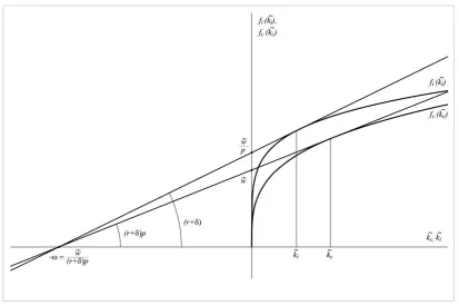
Figure 1 Investment-goods sector and consumption-goods sector production functions in intensive form and their equilibrium state tangents.
The slope of the tangent to the production function in the investment-goods sector fi(k~i)is equal to (r+δ), see Equation (4).
The ordinate of the point of intersection of the tangent to the production function in the investment-goods sector fi(k~i)with the vertical axis is equal to fi(0)=w~/p, see Equation (2). Then the abscissa of the intersection point of the tangent with the horizontal axis is equal to:4
–ω=– [w~/p]/[fi(k~i)/k~i]=–w~ /[(r+δ)p]
Similarly, the slope of the tangent to the production function in the consumption-goods sector is equal tofc(k~c)/k~c p(r), see Equation (3).
The ordinate of the point of intersection of the tangent with the vertical axis is equal to )
0 (
c
f =w~ , see Equation (1).
Then the abscissa of the intersection point of the tangent with the horizontal axis is also equal to:
–ω=–w~ /[fc(k~c)/k~c]=–w~ /[(r + δ)p]
Let us assume (as it is usually done when considering the two-sector growth model with flexible technology), that the production functions in the both industrial sectors are neoclassical and are stationary in the absence of technological progress. Then the common point of intersection of the two tangents with the horizontal axis (its abscissa is equal to –ω=–w~ /[(r + δ)p]) uniquely determines the actual points on the production functions in a state of economic equilibrium.
Consequently, not only the actual equilibrium values of the both capital intensities k~iandk~care determined, but also the values of each of the three variables that determine the value of ω:
w~ - is the ordinate of the point of intersection of the tangent to the consumer-goods function with
the vertical axis;
(r + δ) – is the angle of the tangent to the investment-goods function;
p – is the ratio of the tangent to the consumer-goods function, p(r + δ), to the tangent to the investment-goods function (r + δ) (or the ratio of the ordinates of points of intersection with the vertical axis tangent to the consumer-goods function w~ and the tangent to the investment-good
function w~ /p).
Thus, changing of the operating point (equilibrium state varying) will inevitably lead to the change of the prices ratio p.5
2.2.
Flexible technology with Cobb-Douglas production functions
Let us consider a specific case when flexible technology described by the Cobb-Douglas production functions. The functions can be written in the intensive form:
c c c c
c k A k
f (~) (~) (9)
i i i i
i k A k
f (~) (~) (10)
Let us express the output and the capital intensity in the industrial sectors explicitly as functions of the profit rate. For the investment-goods sector, using the equation (4) and (10), we get:
1
)
~
(
)
(
~
/
)
~
(
ii i i i
i
i
k
k
r
A
k
f
,which implies that
) 1 /( 1
)]
/(
[
)
(
~
ir
A
r
k
i
i
i
(11)) 1 /( )
1 /( 1
)]
/(
[
))
(
~
(
)
(
))
(
~
(
k
r
g
r
A
k
r
iA
ir
i if
i i
i
i i
i
i
(12)Similarly, for the consumer-goods sector, using Equations (3) and (9), we get:
1
)
~
(
)
(
~
/
)
~
(
ci c c c
c
c
k
k
p
r
A
k
f
After expressing the value of p in the last equation by using Equation (6) and the values of k~i(r)
and fi(k~i(r)) - by using Equations (11) and (12) we obtain
}
)]
/(
[
~
)(
(
)]
/(
[
/{
)
~
(
)
(
))
~
~
)(
(
/(
)
(
)
~
(
) 1 /( )
1 /( )
1 /( 1 1
i i i
i i
c c
r
A
k
r
r
A
k
A
r
k
k
r
f
f
r
k
A
i i c i
i c
c
i c i
c i
c c
5 Adjustment of the abscissa of the intersection point can be avoided, if we choose the investment goods (rather than
Solving the resulting equation for the value of capital intensityk~c(r), we obtain an explicit formula for this value as a function of the profit rate:
) 1 /( 1
]
)
(
[
)
1
(
)
1
(
)
(
~
ir
A
r
k
i ic i i c c
(13)Then with the help of Equation (9) we can obtain the value of output in the consumer goods
sector
f
c(
k
~
c(
r
))
as an explicit function of the profit rate:) 1 /(
]
)
(
[
}
)
1
(
)
1
(
{
)
~
(
)
(
))
(
~
(
c c c ir
A
A
k
A
r
g
r
k
f
i ic i i c c c c c c c
(14)The ratio of capital-intensities in both production sectors is a constant in this case, Equations (11) and (13) gives:
) 1 ( ) 1 ( ~ / ~ c i i c i c k k (15)
The value of real wagesw~ also can be expressed explicitly as a function of r. Substituting in the Equation (5) the values of k~i(r), ( ))
~ (k r
fi i ,k~c(r)and fc(k~c(r)) from the Equations (11) - (14) and performing calculations, we obtain:
c c i i c i i c c c f r A A r
w c ] c i (1 )
) ( [ ] ) 1 ( ) 1 ( [ ) 1 ( ) (
~ /(1 )
(16)
The latter equation shows that the value of αc is the share of capital income in the sector
producing consumer goods.
Similarly, we can express the prices ratio p explicitly as a function of r. Substituting in the Equation (6) the values of k~i(r), ( ))
~ (k r
fi i ,k~c(r)and fc(k~c(r)) from the Equations (11) - (14) and performing calculations, we obtain:
) 1 /( ) ( ) 1 /( ) 1 ( ) 1 ( ) ( ) ( ] ) 1 ( ) 1 ( [ )
(r A c A c i r c i i
p i i
i c c i c c
(17)
Note that the model will be closed only if the total income distribution is specified. Let us assume that that the investment and profits are directly proportional:
K r s
Y~i c( )~ (18)
where sc – is a coefficient characterizing the level of reinvestment. Equation (18) is equivalent to
Equation (19)6
(r+δ)=(g+δ)/sc (19)
6
Indeed, one can multiply the left and right sides of the Equation (19) by the amount of capital stock K, and using the obvious formula I=(g+δ)K (equivalent of the Harrod-Domar equation (Harrod,1939; Domar, 1946) obtain I= sc(r+δ)K (where I is the aggregate nominal investment, I
=PiY~i). By dividing the left and right sides of the last equation by the price of capital goods Pi,
the Equation (18) actually comes out.
Let us denote λc≡Lc/L and λi≡Li/L, and λi + λc =1 obviously. Then Equation (18) can be
transformed by dividing the left and right sides by Li:
] / ) 1 ( ~ ~ )[ ( / ) ~ ~ )(
( i c i c i c i i
c
i s r K K L s r k k
f
Solving this equation with respect to λi, obtain:
)) ~ ~ )( ( /( ~ )
( c i c c i
c
i s r k f s r k k
(20) )) ~ ~ )( ( /( )) ( ~ (
1 i i c i i c c i
c f s k r f s r k k
(21)
Substituting in the Equations (20) and (21) the values ofk~i(r), fi(k~i(r)),k~c(r) and fc(k~c(r)) from the Equations (11) - (14) and performing calculations, we obtain:
)] ( 1 [ ) 1 ( i c c c i c c i s s
(22)
)] ( 1 [ ) 1 )( 1 ( i c c c c i c c s s (23)
It turns out that the shares of the labor involved in the industrial sectors, are constants, they do not depend on the equilibrium state. The shares depend only on the shape of Cobb-Douglas production functions and on the coefficient sc, which characterize the level of reinvestment of the
profit. Such constancy of labor shares seems unlikely. Further, we shall see that these shares are not constants when the technology is fixed (not flexible).
Knowing the distribution of labor, we can determine the aggregate amount of capital and output. )) ~ ~ )( ( /( ~ ~ ~ ~ i c c i c i c c i
ik k fk f s r k k
k (24)
i i c
c pf
f
y
~ (25)
Substituting in the Equations (24) and (25) the values of k~i(r), ( )) ~ (k r
fi i ,k~c(r), ( )) ~ (k r
fc c , p, λi,
λc from the Equations (11)-(14), (17), (22), (23) and performing calculations, we obtain:
) 1 /( 1 ) 1 /( 1 ) ( ) ( )] ( 1 [ ) 1 ( ) ( ~ i i r A s r
k i i
i c c c i i
c
(26)
) 1 /( ) 1 /( ) ( ) ( } )] 1 ( [ ) 1 ( { )] ( 1 [ ) ( 1 )( 1 ( ) (
~ c A c i r c i
s s A
r
y i i
c i i c i c c c i c c c
c
(27)
represented as the Cobb-Douglas function where an exponent of capital αc is equal to the
exponent of capital in the production function for the consumer goods sector:
c
k const k
y(~) ~
~
The amazing fact that the two Cobb-Douglas production functions with different exponents of capital aggregated in the Cobb-Douglas function is easily explained. The both initial production functions should be provided in a unified unit of measurement, to make possible the aggregation. Using as a unit consumer goods as a numeraire, we have to multiply by the price ratio p the production function for the investment goods sector, see Equation (25). The price ratio p depends on profit rate in such a specific way (see Equation 17) that produces adjustment of the function: the product pfi has the same exponent of the profit rate, as a function fc for the consumer goods sector. In addition, if we shall use the consumer good as a numeraire, considering Y~≡Y/Pi, then
we should use the equation ~y fcc/ p fii instead of the Equation (25) for the purpose of aggregation. Easy to see that in this case the appropriate aggregate production function will have the exponent of capital αi, which corresponds to the investment goods sector:
i
k t cons p
k y k
y (~) ~(~)/ ~
~
Thus, although in this case the aggregate production function formally has the right to exist7, but it has not a deep economic sense. The function is inseparably linked with prices ratio p, and therefore it cannot be regarded as a purely technical function.
Whether is there an optimal equilibrium state in the case with a flexible technology? In the present study, the equilibrium state is the best when the aggregate profit received reaches the maximum.8 To find the optimum we must look for the equilibrium state (i.e., the corresponding value of profit rate), which ensures a maximum profit per worker.
The value of profits per unit of labor p(r)k~can be expressed as a function of the profit rate (see Equations 17 and 26). The exponent of profit rate is equal to [1-1/(1-αi)-(αc -αi)/ (1-αi)]=
- αc/(1-αi), then
) 1 /(
) ( ~
)
(r k const r c i
p pr (28)
Profit is a decreasing function of the profit rate. Then the capitalists should reduce profit rate in an attempt to increase their profits. This should result in euthanasia of proprietors. Such a pessimistic scenario is typical for flexible technology in the absence of technological progress. In the next section, we consider the case of fixed technology, with a more interesting dynamic.
3.
Fixed coefficients
Let us consider the case with fixed coefficients, when each sector has its unique fixed production technology9. Technological progress and labor productivity growth are also absent in this case; output grows only due to the population growth and proportional capital accumulation. Consequently, each sector has the technologically specified number of output (consumption or investment goods) that are produced by a single machine per time unit. This number is given and invariable for each sector, as well as the number of employees needed to service one machine. It means that for any equilibrium state the output-to-capital ratio, capital intensity and per-worker
7 A number of economists (Felipe & Fisher, 2003; Shaikh, 1974) already have questioned the existence of the
neoclassical aggregate production function
8 Do not confuse this condition with the condition of profit maximization, when the profit rate is equal to the
marginal product of capital. The latter condition is a "microeconomic", which minimize the costs of firms.
9 The contribution of Stiglitz (1968) justified the assumption about fixed technology: ‘the optimum requires that
output values are fixed and equal to the technologically specified ones, fc=fc*, fi=fi*, k~c k~c,
i
i k
k~ ~ . These quantities are invariable for the different equilibrium states, and such variables are designated by asterisk. Then the Equations (1), (2) can be rewritten:
c
c w p r k
f ~ ( )~ (29)
i
i w p r k
pf ~ ( )~ (30)
We have 2 equations and 3 variables (p, (r+δ),w~ ). Only one of the variables can be independent
(exogenously given). Let us consider the profit rate r as an independent variable, similarly to Section 2. Then the values of w~ and p can be calculated as the functions of r using the solution to the linear system, which involves Equations (29) and (30):
)) ~ ~ )( ( /( ) ~ ) ( (
~
i c i
i i
c f r k f r k k
f
w (31)
)) ~ ~ )( (
/(
fc fi r kc ki
p (32)
The derivatives of w~(r)and p(r) can be calculated by using Equations (31) and (32)
0 )) ~ ~ )( ( /( ~ /
~ 2
i c i
c i
c f k f r k k
f r
w (33)
2
)) ~ ~ )( ( /( ) ~ ~ (
/
p r fc kc ki fi r kc ki (34)
Surprisingly, but the derivatives are equal to the ones which were obtained for the case with flexible technology (see Equations 7 and 8).
Similarly, Equation (33) demonstrates that w~/r is always less than zero, which means an understandable and unceasing fight between wages and profits (the growth of one of the values automatically means a reduction of the second one and vice versa).
Equation (34) demonstrates that ∂p/∂r= 0 only whenk~i k~c. This means that any dynamic two-sector model must take account of changes of the prices ratio (except for the special case when the capital intensities in different sectors are equal, which corresponds to the one-commodity model).
Let us specify the total income distribution. Similarly, to the case with flexible technology we shall assume that that the values of profits and investment are directly proportional (see Equation 18). Then we can calculate the shares of total labor used in different sectors, and aggregate capital and output. Equations (20) and (21) can be rewritten for the case with fixed technology:
)) ~ ~ )( ( /(
~ )
(
c c i c c i
i s r k f s r k k
(35)
)) ~ ~ )( ( /(
)) ( ~ (
1
i i c i i c c i
c f s k r f s r k k
(36)
The labor shares are not constants; they are the functions of r, in contrast to the case with flexible technology. By differentiating with respect to r,
0 )] ~ ~ )( ( /[
~
/ 2
i c c
i i c c
i r s k f f s r k k
(37)
0 )] ~ ~ )( ( /[
~
/ 2
i c c
i i c c
c r s k f f s r k k
The share of total labor used in the consumer-goods industrial sector decreased with an increase of the profit rate. As an illustration of the last property, let us consider an interesting special case of the transition from one equilibrium state to another. Suppose that the population and labor growth rate n changes that results in an alteration of the output growth rate, g= n, without any variations in technology. Then the profit rate r should increase as well (see Eq. 19). More rapid pace of labor growth requires a larger (gross) investment (n+δ) k to maintain technologically specified level of capital intensity. Then the share of workers λi in the investment goods sector
should grow, respectively, the share of workers in the consumption goods sector λc should
decrease (see Inequalities 37 and 38). The lesser share of workers in the consumer-goods sector would produce the lesser consumption goods per capita. This means a lower real consumption (see Equation 33), and the lower (real) wage in terms of the consumer goods. The result is that
the rapid population growth is “disadvantageous” in terms of consumption maximization.
If the distribution of labor across sectors (see Equations 35 and 36) is known, then the aggregate capital-labor ratio k~ can be calculated:
)) ~ ~ )( ( /(
~ ~
~
~
i c c
i c i c c i
ik k f k f s r k k
k (39)
By differentiating,
2
)) ~ ~ )( ( /(
) ~ ~ ( ~ /
~
k r fi kcsc kc ki fi sc r kc ki (40)
The aggregate output in intensive form ~y in terms of consumer goods is equal to
i i c
c pf
f
y
~ (41)
Substituting the equilibrium values of λi and λc from Equations (35) and (36), and the value of
the price ratio p from Equation (32) in Equation (41), one can calculate in explicit form the function of aggregate output ~y ~y(r) as a function of the profit rate (we will not reproduce here this expression because of its unwieldiness). Differentiating the resulting function of aggregate output ~y(r) by r yields:
2 ))] ~ ~ )( ( ))( ~ ~ )( ( [(
/ )] ~ ~ )( 1 )( ( 2 )[ ~ ~ ( ~ /
~
i c i
i c c
i
i c c i
i c c c c i
k k r f k k r s f
k k s r
f k k s k f f r y
(42)
Note that despite the fact that the technology in both sectors is fixed (i.e. discrete), the aggregate capital intensity and the aggregate output are continuous and differentiable functions in the domain of definition (k~i k~k~c). The properties of the function of aggregate output thoroughly discussed below.
3.1.
Fixed coefficients. Uzawa capital intensity condition and properties
of the function of aggregate output
Equations (34), (40) and (42) show the possibility of two different opportunities: the violation or fulfillment of the Uzawa capital-intensity condition:
(а) k~i k~c
(б) k~i k~c
∂p/∂r > 0 (see Equation 34) 0
/ ~
k r (see Equation 40) 0
/ ~
y r (see Equation 42)
Variant (a) is intrinsically unstable; it is shown strictly at the end of this section. All three derivatives are greater than zero. If the profit rate r is growing, then all three factors that directly affect profit (per employee) should grow as well (r×p× k~). Since the capitalists aspire to maximize profits, they will seek to further growth of the profit rate. This means positive feedback and instability. Theoretically, the profit rate in this case could grow to such an extent that the capital income share would absorb the entire gross income, reducing to zero the labor income share. Of course, such a perspective is not possible; growth of the capital income share is limited by the lowest possible subsistence wages. This situation could take place in the early capitalism, during the primary accumulation of capital. For a long time during this period, the salary was remaining at the level of subsistence wages, so the classical economists (e.g. Ricardo, 1817) considered the constancy of wages at this level as a fundamental assumption.
(b) Uzawa condition met, k~i k~c, such inequality is typical for modern economies. Then ∂p/∂r < 0 (see Equation 34)
0 / ~
k r (see Equation 40) 0
/ ~
y r (see Equation 42)
In this case, all three derivatives are negative. If the profit rate r is growing, then not only labor productivity y~ decreases, but also aggregate capital intensity k~ and price ratio p – the factors that directly affect real profit. This property provides the negative feedback and ensures the stability of the equilibrium state. It is shown strictly below: under Uzawa capital-intensity condition the resulting function of aggregate output has the properties of the neoclassical production function, i.e. diminishing returns of capital, and then the equilibrium state is stable. The unwieldy dependence~y ~y(r), which can be obtained from Equation (41) above can be represented also in the usual trivial form (anyone can make it by substituting formulas for the values of wage w~ (Equation 31) and for the aggregate capital intensity k~ (Equation 39)):
k r p w
y ~ ( )~
~ (43)
The first derivative is obviously:
0 ) ( ~ / ~
y k p r (44)
The second derivative can be calculated as follows: taking into account thatk~k~(r),
r k k y r k y / ~ ) ~ / ~ ( ) ~ / ~
( 2 2
Then by using Equations (32), (34) and (40) for the values of p, ∂p/∂r, ∂k~/∂r, obtain:
0 ~ / ~ 2 2
y k if k~i k~c and 2~y/k~2 0 if k~i k~c (45)
Equations (44) and (45) indicate that the function of aggregate output (for the model with fixed technology) has the properties of the neoclassical production function, including diminishing returns of capital, only under Uzawa capital-intensity condition. If this condition is not met, then the increasing return of capital occurs which is accompanied by instability of the equilibrium state. That is, in this model Uzawa capital-intensity criterion is a necessary condition for the stability of the equilibrium state. Moreover, it will be shown in the next section, that the model demonstrates the possibility of existence of an optimal equilibrium state, ensuring maximum profit.
3.2.
Existence of the optimal equilibrium state with maximum profit
In this Section we show, that within the present model (with fixed coefficients) under certain conditions the optimal equilibrium state may exist, when the function of profit has a maximum. It is advantageous for the capitalists to maximize the total per employee profits, i.e., the valueof p(r)k~. Let us substitute the value of p from Equation (32) and the value of k~from Equation (39), and differentiate the product:
2 2 2
2
))] ~ ~ )( ( ))( ~ ~ )( ( [(
/ ] ) ~ ~ ( ) ( ) [( /
) ~ ) ( (
i c i
i c c
i
i c c i
c i
k k r f k k r s f
k k s r
f f f r k r p
(46)
Equating the derivative to zero to find the extremum, (p(r)k~)/r 0, one can obtain:
)] ~ ~ (
/[ c c i
i
extr f s k k
r (47)
It is clear from Equation (46) that (p(r)k~)/r0 (profit rises when profit rate grows) when r< rextr, and vice versa, (p(r)k~)/r0 (profit decreases when profit rate grows)
when r> rextr. Therefore, the value of which is obtained in Equation (47) corresponds to the
maximum of the profit functionp(r)k~, rextr= rmax. Therefore, the equilibrium state is optimal
for capitalists when r= rmax.
In the case (a), when Uzawa capital-intensity condition is not met (k~i k~c), it follows from the obvious inequality (rmax+δ)>0 that the only one possible positive root of the Equation (47) is:
)] ~ ~ ( /[
max fi sc ki kc r
This maximum point is not meaningful and cannot exist, since this will be negative one of the two values: either the share of workers in the investment sectorλi(rmax), or the price ratio p(rmax). It is shown below.
The share of workers in the investment sector for the optimal equilibrium state λi(rmax) is equal (see Equation 35):
)] ~ ~ )( 1
/[( ~ ))
~ ~ )( (
~ /( ~ ) (
)
( max c max c i i c max c i c c c i c
i r s r k k q s r k k s k s k k
The obvious inequalityλi(rmax)>0 should be carried out, then the condition sc <1 follows from the
last equation.
] ) / 1 1 /[( ))
~ ~ )( (
/( )
(rmax fc fi rmax kc ki fc sc fi
p
It requires sc >1 to comply with another obvious condition p(rmax)>0.
Have a contradiction: the two required conditions cannot be satisfied simultaneously. Consequently, r*
max value is outside the range of admissible values of the profit rate in the case
(a), whenk~i k~c. Therefore, a maximum of profit function does not exist in the case (a).
In the case (b), when Uzawa capital-intensity condition complied (k~i k~c), the only one possible positive root of the Equation (47) is:
)] ~ ~ ( /[
max fi sc kc ki
r (48)
In this case, the maximum of profit function p(r)k~can exist only if the capital intensity kc
~
in the sector, producing consumer products is quite large (relativelyk~i). It follows from the two obvious conditions.
The first condition is λi <1. Substituting in the Equation (35) the value of rmax from the Equation (48), obtain:
1 )] ~ ~ )( 1
/[( ~ ))
~ ~ )( (
/( ~ ) (
)
( max c max c i c max c i c c c c i
i r s r k f s r k k s k s k k
or
i c
c s k
k~ (1 )~ (49а)
The second condition, w>0, gives obvious inequality (r+δ)k~i< fi* (see Eq. 31). Substituting the value of rmax from the Eq. (48) in this inequality, obtain:
c i c
c s k s
k~ (1 )~/ (49b)
3.3.
Allowance for labor productivity growth
In this section, we allow the technological progress and labor productivity growth at a constant rate η. First, consider a model with fixed technology. Let us assume in this case, that new and more efficient technologies in each of the industrial sectors have the same capital-to-output ratios as the old ones. The assumption means that the output-to-capital ratios in each industrial sector are not dependent of time:
i i i i i i
i
i t K t f t k t f k f k
Y~( )/ ~( ) ( )/~( ) (0)/~(0) /~
c c c c c c
c
c t K t f t k t f k f k
Y~( )/ ~ ( ) ( )/~( ) (0)/~(0) /~
At the same time, the values of capital intensity and labor productivity grow at the constant equal rateη. Thus the equilibrium growth rate of the total output will be equal to the sum of the growth rate of labor productivity and the growth rate of population g=n + η. The initial (starting) values of capital intensity and labor productivity are given.
) exp( ~ ) exp( ) 0 ( ~ ) ( ~
t k
t k
t
ki i i
) exp( ~ ) exp( ) 0 ( ~ ) ( ~
t k
t k
t
kc c c
) exp( )
exp( ) 0 ( )
(t f t f t
fi i
i
)
exp(
)
exp(
)
0
(
)
(
t
f
t
f
t
f
c
c
c
The amount of wage increases exponentially at the same rate as labor productivity (otherwise the labor share in the total income would change).
) exp( ~ ) exp( ) 0 ( ~ ) (
~ t w t w t
Substituting the above values in the Equations (31), (32), (35), (36), (39) and (41) shows that these equations can be reduced by dividing both sides by the exponential factor, exp (ηt). Then the equations become stationary and equivalent with the equations obtained in the absence of labor productivity growth. Thus, none obtained above (in Section 3) results should change if the labor productivity growth at a constant rate takes place.
The same logic can be used to show that technological progress (and labor productivity growth) maintaining a constant rate of capital-output ratio does not affect the conclusions in the case of the flexible technology.
4.
Conclusion
This paper reexamined the two-sector growth model for 2 cases: with flexible technology or with fixed coefficients. Only one of the variables may be independent, we adopted the profit rate as such a variable. That is, we assume that the equilibrium state (when the factor prices do not differ across sectors and are equal to the marginal products) is determined by this value. The remaining variables are treated as functions of the profit rate.
The comparative analysis of different equilibrium states within the two-sector growth model shows correlations, which are common for the both cases:
-Understandable and unceasing fight between the prices of the main factors of production (wage and profit rate), see Inequalities (7) and (33). Growth of one of the values automatically means a decrease of the other.
- The inevitable change of the investment-good price to consumer-good price ratio, if the equilibrium state has changed, see Equations (8) and (34). An exception, when the price ratio maintained, is the unlikely special case when the capital intensities in different sectors are equal,
c
i k
k~ ~ , which corresponds to the one-commodity model. Then any dynamic model, which considers more than one sector, must take into account changes in the price ratio.
The assumption about direct proportionality between profits and investment specifies the distribution of total income for both cases in the paper. It makes possible to calculate the distribution of labor and capital between sectors and to derive the aggregate production function. If the technologies are flexible and described by Cobb-Douglas production functions, then the labor shares are constants, they are not dependent from r. Surprisingly, the aggregate production function also has Cobb-Douglas form. The dependence p(r) has a specific form, and it makes possible to aggregate two Cobb-Douglas functions with different values of exponent of capital. Therefore, the aggregate production function is not purely technical.
The dynamics become more interesting if we consider the model with fixed technology:
- The labor force moves toward the investment sector if the profit rate increases, see Inequalities (37) and (38). An interesting conclusion is shown: the negative impact of the high rate of population growth on the per capita consumption.
- The aggregate values of capital intensity and output are continuous functions within obvious limitations (k~ik~k~c), despite the fact that the capital intensities and labor productivities in the industrial sectors are fixed (discrete). The function of aggregate output under Uzawa capital-intensity condition (k~i k~c) has the properties of the neoclassical production function, including diminishing returns of capital. This ensures the stability of the equilibrium state, unlike the instability that occurs if Uzawa condition is not met.
References
Acemoglu D. (2008) Introduction to Modern Economic Growth, Princeton University Press.
Corden W. M., (1966) “The two sector growth model with fixed coefficients,” The Review of Economic Studies, vol. 33, no. 3, pp. 253–262.
Domar E. D. (1946) “Capital Expansion, Rate of Growth, and Employment”, Econometrica,
14(4), 137 – 147.
Felipe J., Fisher F. M. (2003) “Aggregation in Production Functions: What Applied Economists Should Know”, Metroeconomica, 54(2-3), 208-262.
Harrod R. F. (1939) “An Essay on Dynamic Theory”, Economic Journal, 49 (193), 14 – 33.
Kaldor, N. (1955-1956), “Alternative theories of distribution”, The Review of Economic Studies, 23, 94-100.
________. (1963) “Capital Accumulation and Economic Growth”. In Friedrich A. Lutz and
Douglas C. Hague, eds., Proceedings of a Conference Held by the International Economic Association. London: Macmillan.
Keynes J. M. (1936) The General Theory of Employment, Interest, and Money, New York: Harcourt.
Pasinetti L. (1962) “Rate of Profit and Income Distribution in Relation to the Rate of Economic
Growth”, Review of Economic Studies 29(4), 267–79.
________. (2000) “Critique of the Neoclassical Theory of Growth and Distribution”, Banca Nazionale del Lavoro Quarterly Review, 53(215), 383—431.
Phelps, E. S. (1961) “The Golden Rule of Accumulation: A fable for growthmen”, American Economic Review, 51, 638-643.
Ramsey, F. (1928) “A Mathematical Theory of Savings", Economic Journal, Vol. 38, pp. 543-559.
Ricardo, D., [1817], (1951), On the Principles of Political Economy and Taxation, P. Sraffa, ed.
with the collaboration of M. Dobb, “The Works and Correspondence of David Ricardo”,
Cambridge, Cambridge University Press.
Shaikh A. (1974) “Laws of Production and Laws of Algebra: The Humbug Production Function”, Review of Economics and Statistics, 56(1), 115-120.
Solow, Robert M. (1956) “A Contribution to the Theory of Economic Growth”, Quarterly Journal of Economics, 70, 65–94.
Sraffa P. (1960) “Production of Commodities by Means of Commodities: a Prelude to a critique
of Economic Theory”, Cambridge, Cambridge University Press.
Stiglitz, J. E. (1968) “A Note on Technical Choice under Full Employment in a Socialist
Stolper, W. F.; Samuelson, Paul A. (1941). "Protection and real wages", The Review of Economic Studies. Vol. 9 (1): 58–73.
Swan T.W. (1956) “Economic Growth and Capital Accumulation”, Economic Record, 32 (2), 334–361.
Uzawa H. (1961a) “Neutral Inventions and the Stability of Growth Equilibrium,” Review of Economic Studies, 28(2), 117-124.
________. (1961b) "On a Two-Sector Model of Economic Growth, I", Review of Economic Studies, 29, 40-47.
________. (1963) "On a Two-Sector Model of Economic Growth, II", Review of Economic Studies, 30, 105-118.