Transition Based Parsing for Deep Dependency Structures

Dependency Structures

Xun Zhang

Yantao Du

Weiwei Sun

Xiaojun Wan

Derivations under different grammar formalisms allow extraction of various dependency struc-tures. Particularly, bilexical deep dependency structures beyond surface tree representation can be derived from linguistic analysis grounded byCCG,LFG, andHPSG. Traditionally, these dependency structures are obtained as a by-product of grammar-guided parsers. In this arti-cle, we study the alternative data-driven, transition-based approach, which has achieved great success for tree parsing, to build general dependency graphs. We integrate existing tree pars-ing techniques and present two new transition systems that can generate arbitrary directed graphs in an incremental manner. Statistical parsers that are competitive in both accuracy and efficiency can be built upon these transition systems. Furthermore, the heterogeneous design of transition systems yields diversity of the corresponding parsing models and thus greatly benefits parser ensemble. Concerning the disambiguation problem, we introduce two new techniques, namely, transition combination and tree approximation, to improve parsing quality. Transition combination makes every action performed by a parser significantly change configurations. Therefore, more distinct features can be extracted for statistical disambiguation. With the same goal of extracting informative features, tree approximation induces tree backbones from dependency graphs and re-uses tree parsing techniques to produce tree-related features. We conduct experiments onCCG-grounded functor–argument analysis,LFG-grounded grammatical relation analysis, andHPSG-grounded semantic dependency analysis for English and Chinese. Experiments demonstrate that data-driven models with appropriate transition systems can produce high-quality deep dependency analysis, comparable to more complex grammar-driven

∗The authors are with the Institute of Computer Science and Technology, the MOE Key Laboratory of Computational Linguistics, Peking University, Beijing 100871, China.

E-mail:{zhangxunah,duyantao,ws,wanxiaojun}@pku.edu.cn.Weiwei Sun is the corresponding author. Submission received: 6 May 2015; revised submission received: 2 November 2015; accepted for publication: 18 January 2016.

models. Experiments also indicate the effectiveness of the heterogeneous design of transition systems for parser ensemble, transition combination, as well as tree approximation for statistical disambiguation.

1. Introduction

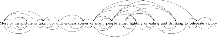
The derivations licensed by a grammar under deep grammar formalisms, for example, combinatory categorial grammar (CCG; Steedman 2000), lexical-functional grammar (LFG; Bresnan and Kaplan 1982) and head-driven phrase structure grammar (HPSG; Pollard and Sag 1994), are able to produce rich linguistic information encoded as bilexical dependencies. UnderCCG, this is done by relating the lexical heads of functor categories and their arguments (Clark, Hockenmaier, and Steedman 2002). UnderLFG, bilexical grammatical relations can be easily derived as the backbone of F-structures (Sun et al. 2014). UnderHPSG, predicate–argument structures (Miyao, Ninomiya, and ichi Tsujii 2004) or reduction of minimal recursion semantics (Ivanova et al. 2012) can be extracted from typed feature structures corresponding to whole sentences. Dependency analysis grounded in deep grammar formalisms is usually beyond tree representations and well-suited for producing meaning representations. Figure 1 is an example from CCGBank. The deep dependency graph conveniently represents more semantically motivated information than the surface tree. For instance, it directly captures the

Agent–Predicaterelations between word “people” and conjuncts “fight,” “eat,” as well as “drink.”

Automatically building deep dependency structures is desirable for many practical NLP applications, for example, information extraction (Miyao et al. 2008) and question answering (Reddy, Lapata, and Steedman 2014). Traditionally, deep dependency graphs are generated as a by-product of grammar-guided parsers. The challenge is that a deep-grammar-guided parsing model usually cannot produce full coverage and the time complexity of the corresponding parsing algorithms is very high. Previous work on data-driven dependency parsing mainly focused on tree-shaped representations. Nevertheless, recent work has shown that a data-driven approach is also applicable to generate more general linguistic graphs. Sagae and Tsujii (2008) present an initial study on applying transition-based methods to generateHPSG-style predicate–argument structures, and have obtained competitive results. Furthermore, Titov et al. (2009) and Henderson et al. (2013) have shown that more general graphs rather than planars can be produced by augmenting existing transition systems.

This work follows early encouraging research and studies transition-based ap-proaches to construct deep dependency graphs. The computational challenge to in-cremental graph spanning is the existence of a large number of crossing arcs in deep

Figure 1

dependency analysis. To tackle this problem, we integrate insightful ideas, especially the ones illustrated in Nivre (2009) and G ´omez-Rodr´ıguez and Nivre (2010), developed in the tree spanning scenario, and design two new transition systems, both of which are able to produce arbitrary directed graphs. In particular, we explore two techniques to lo-calize transition actions to maximize the effect of a greedy search procedure. In this way, the corresponding parsers for generating linguistically motivated bilexical graphs can process sentences in close to linear time with respect to the number of input words. This efficiency advantage allows deep linguistic processing for very-large-scale text data.

For syntactic parsing, ensembled methods have been shown to be very helpful in boosting accuracy (Sagae and Lavie 2006; Zhang et al. 2009; McDonald and Nivre 2011). In particular, Surdeanu and Manning (2010) presented a nice comparative study on various ensemble models for dependency tree parsing. They found that the diversity of base parsers is more important than complex ensemble models for learning. Motivated by this observation, the authors proposed a hybrid transition-based parser that achieved state-of-the-art performance by combining complementary prediction powers of different transition systems. One advantage of their architecture is the linear-time decoding complexity, given that all base models run in linear-time. Another concern of our work is about the model diversity obtained by the heterogeneous design of transition systems for general graph spanning. Empirical evaluation indicates that statistical parsers built upon our new transition systems as well as the existing best transition system—namely, Titov et al. (2009)’s system (THMM, hereafter)—exhibit complementary parsing strengths, which benefit system combination. In order to take advantage of this model diversity, we propose a simple yet effective ensemble model to build a better hybrid system.

We implement statistical parsers using the structured perceptron algorithm (Collins 2002) for transition classification and use a beam decoder for global inference. Concern-ing the disambiguation problem, we introduce two new techniques, namely, transition combination and tree approximation, to improve parsing quality. To increase system coverage, the ARC transitions designed by theTHMM as well as our systems do not change the nodes in the stack nor buffer in a configuration: Only the nodes linked to the top of the stack or buffer are modified. Therefore, features derived from the config-urations before and after an ARCtransition are not distinct enough to train a good clas-sifier. To deal with this problem, we propose the transition combination technique and three algorithms to derive oracles for modified transition systems. When we apply our models to semantics-oriented deep dependency structures, for example,CCG-grounded functor–argument analysis andHPSG-grounded reduced minimal recursion semantics (MRS; Copestake et al. 2005) analysis, we find that syntactic trees can provide very helpful features. In case the syntactic information is not available, we introduce a tree approximation technique to induce tree backbones from deep dependency graphs. Such tree backbones can be utilized to train a tree parser which provides pseudo tree features. To evaluate transition-based models for deep dependency parsing, we conduct experiments onCCG-grounded functor–argument analysis (Hockenmaier and Steedman 2007; Tse and Curran 2010),LFG-grounded grammatical relation analysis (Sun et al. 2014), andHPSG-grounded semantic dependency analysis (Miyao, Ninomiya, and ichi Tsujii 2004; Ivanova et al. 2012) for English and Chinese. Empirical evaluation indicates some non-obvious facts:

1. Data-driven models with appropriate transition systems and

2. Parsers built upon heterogeneous transition systems and decoding orders have complementary prediction strengths, and the parsing quality can be significantly improved by system combination; compared to the best individual system, system combination gets an absolute labeled F-score improvement of 1.21 on average.

3. Transition combination significantly improves parsing accuracy on a wide range of conditions, resulting in an absolute labeled F-score improvement of 0.74 on average.

4. Pseudo trees contribute to semantic dependency parsing (SDP) equally well to syntactic trees, and result in an absolute labeled F-score

improvement of 1.27 on average.

We compare our parser with representative state-of-the-art parsers (Miyao and Tsujii 2008; Auli and Lopez 2011b; Martins and Almeida 2014; Xu, Clark, and Zhang 2014; Du, Sun, and Wan 2015) with respect to different architectures. To evaluate the impact of grammatical knowledge, we compare our parser with parsers guided by treebank-induced HPSG and CCG grammars. Both of our individual and ensembled parsers achieve equivalent accuracy to HPSGand CCGchart parsers (Miyao and Tsujii 2008; Auli and Lopez 2011b), and outperform a shift-reduceCCGparser (Xu, Clark, and Zhang 2014). It is worth noting that our parsers exclude all syntactic and grammatical information. In other words, strictly less information is used. This result demonstrates the effectiveness of data-driven approaches to the deep linguistic processing prob-lem. Compared to other types of data-driven parsers, our individual parser achieves equivalent performance to and our hybrid parser obtains slightly better results than factorization parsers based on dual decomposition (Martins and Almeida 2014; Du, Sun, and Wan 2015). This result highlights the effectiveness of the lightweight, transition-based approach.

Parsers based on the two new transition systems have been utilized as base com-ponents for parser ensemble (Du et al. 2014) for SemEval 2014 Task 8 (Oepen et al. 2014). Our hybrid system obtained the best overall performance of the closed track of this shared task. In this article, we re-implement all models, calibrate features more carefully, and thus obtain improved accuracy. The idea to extract tree-shaped backbone from a deep dependency graph has also been used to design other types of parsing models in our early work (Du et al. 2014, 2015; Du, Sun, and Wan 2015). Nevertheless, the idea to train a pseudo tree parser to serve a transition-based graph parser is new.

The implementation of our parser is available athttp://www.icst.pku.edu.cn/

lcwm/grass.

2. Transition Systems for Graph Spanning

2.1 Background Notations

A dependency graphG=(V,A) is a labeled directed graph, such that for sentencex= w1,. . .,wnthe following holds:

1. V={0, 1, 2,. . .,n},

The vertex setVconsists ofn+1 nodes, each of which is represented by a single integer. In particular, 0 represents a virtual root nodew0, and all others correspond to words in

x. The arc setArepresents the labeled dependency relations of the particular analysis

G. Specifically, an arc (i,r,j)∈A represents a dependency relationr from head wi to dependentwj. A dependency graphGis thus a set of labeled dependency relations be-tween the root and the words ofx. To simplify the description in this section, we mainly consider unlabeled parsing and assume the relation setRis a singleton. Or, taking it another way, we assumeA⊆V×V. It is straightforward to adapt the discussions in this article for labeled parsing. To do so, we can parameterize transitions with possible dependency relations. For empirical evaluation as discussed in Section 5, we will test both labeled and unlabeled parsing models.

Following Nivre (2008), we define a transition system for dependency parsing as a quadrupleS=(C,T,cs,Ct), where

1. Cis a set of configurations, each of which contains a bufferβof (remaining) words and a setAof dependency arcs,

2. Tis a set of transitions, each of which is a (partial) functiont:C→C, 3. csis an initialization function, mapping a sentencexto a configuration

withβ=[1,. . .,n],

4. Ct⊆Cis a set of terminal configurations.

Given a sentencex=w1,. . .,wnand a graphG=(V,A) on it, if there is a sequence of transitionst1,. . .,tm and a sequence of configurationsc0,. . .,cmsuch thatc0=cs(x),

ti(ci−1)=ci(i=1,. . .,m),cm∈Ct, andAcm =A, we say the sequence of transitions is an

oraclesequence. And we define ¯Aci =A−Aci for the arcs to be built ofci. We could

denote a transition sequence as either t1,mor c0,m.

In a typical transition-based parsing process, the input words are put into a queue and partially built structures are organized by a stack. A set of SHIFT/REDUCEactions are performed sequentially to consume words from the queue and update the partial parsing results organized by the stack. Our new systems designed for deep parsing differ with respect to their information structures to define a configuration and the behaviors of transition actions.

2.2 Naive Spanning and Locality

For every two nodes, a simple graph-spanning strategy is to check if they can be directly connected by an arc. Accordingly, a “naive” spanning algorithm can be implemented by exploring a left-to-right checking order, as introduced by Covington (2001) and modified by Nivre (2008).

PARSE(x=(w1,. . .,wn)) 1 forj=1..n

2 fork=j−1..1 3 Link(j,k)

LEFT-ARC (σ|i,j|β)⇒(σ|i,j|β) RIGHT-ARC (σ|i,j|β)⇒(σ|i,j|β) SHIFT (σ,j|β)⇒(σ|j,β) POP (σ|i,β)⇒(σ,β) SWAP (σ|i|j,β)⇒(σ|j,i|β) SWAPT (σ|i|j,β)⇒(σ|j|i,β)

Figure 2

Transitions of the online re-ordering approach.

The complexity of naive spanning is θ(n2_),1 _{because it does nothing to explore}

the topological properties of a linguistic structure. In other words, the naive graph-spanning idea does not fully take advantages of the greedysearch of the transition-based parsing architecture. On the contrary, a well-designed transition system for (projective) tree parsing can decode in linear time by exploiting locality among subtrees. Take the arc-eager system presented in Nivre (2008), for example: Only the nodes at the top of the stack and the buffer are allowed to be linked. Such limitation is the key to implement a linear time decoder. In the following, we introduce two ideas to localize a transition action, that is, to allow a transition to manipulate only the frontier items in the data structures of a configuration. By this means, we can decrease the number of possible transitions for each configuration and thus minimize the total decoding time.

2.3 System 1: Online Re-ordering

The online re-ordering approach that we explore is to provide the system with ability to re-order the nodes during parsing in an online fashion. The key idea, as introduced in Titov et al. (2009) and Nivre (2009), is to allow a SWAPtransition that switches the position of the two topmost nodes on the stack. By changing the linear order of words, the system is able to build crossing arcs for graph spanning. We refer to this approach as online re-ordering. We introduce a stack-based transition system with online re-ordering for deep dependency parsing. The obtained oracle parser is complete with respect to the class of all directed graphs without self-loop.

2.3.1 The System.We define a transition systemSS=(C,T,cs,Ct), where a configuration

c=(σ,β,A)∈Ccontains a stackσof nodes, besidesβandA. We set the initial configu-ration for a sentencex=w1,. . .,wnto becs(x)=([], [1,. . .,n],{}), and takeCtto be the set of all configurations of the formct=(σ, [],A) (for anyσanyA). These transitions are shown in Figure 2 and explained as follows.

r

r

whereiis the top of the stack, andjis the front of the buffer.

r

r

A variation of transition SWAP is SWAPT, which updates the configuration by

swappingiandj. However, the system of this variation is not complete with respect to directed graphs because the power of transition SWAPTis limited, and counterexamples

of completeness can be found. For more theoretical discussion about this system (i.e., THMM), see Titov et al. (2009). We also denote Titov et al. (2009)’s system asST.

2.3.2 Theoretical Analysis.The soundness ofSSis trivial. To demonstrate the completeness of the system, we give a constructive proof that can derive oracle transitions for any arbitrary graph. To simplify the description, the label attached to transitions are not considered. The idea is inspired by Titov et al. (2009). Given a sentencex=w1,. . .,wn and a graph G=(V,A) on it, we start with the initial configuration c0 =cs(x) and compute the oracle transitions step by step. On thei-th step, letp be the top ofσci−1, bbe the front ofβci−1; letL(j) be the ordered list of nodes connected tojin ¯Aci−1for any

nodej∈σci−1; letL(σci−1)=[L(j0),. . .,L(jl)] ifσci−1=[jl,. . .,j0].

The oracle transition for each configuration is derived as follows. If there is no arc linked topin ¯Aci−1, then we setti topop; if there existsa∈A¯ci−1 linkingp andb, then

we settitolaorracorrespondingly. When there are onlyshandswleft, we see if there is any nodequnder the top ofσci−1 such thatL(q) precedesL(p) by the lexicographical

order. If so, we settitosw; else we settitosh. An example for when to doswis shown in Figure 3. Letci=ti(ci−1); we continue to computeti+1, untilβciis empty.

Lemma 1

Iftiissh,L(σci−1)=[L(j0),. . .,L(jl)] is complete ordered by lexicographical order.

Proof

It cannot be the case that for someu>0,L(ju) strictly precedesL(j0), otherwisetishould besw. It also cannot be the case that for some u>v>0, L(ju) strictly precedesL(jv), because whenjv−1 is shifted onto the stack,L(jv) precedesL(ju) and all the transitions do not changeL(jv) andL(ju) afterwards.

Lemma 2

Fori=0,. . .,m, there is no arc (j,k)∈A¯cisuch thatj,k∈σi.

Proof

Whenj∈σci is shifted onto the stack by thew-th transitiontw, there must be no arc

(j,k) or (k,j) in ¯Acw such thatk∈σcw. Otherwise, by induction every node inσcw−1 can

only link to nodes inβcw−1, which implies thatL(k) has one of the smallest

lexicograph-ical orders, and from Lemma 1 the top ofσcw−1must be linked toj. And notsh, butlaor rashould be applied.

Figure 3

σ,β, and ¯Aof two configurationsc1andc2. In the left graphic,L(σc1)=[[6], [5], [5, 6], [7]].

Theorem 1

t1,. . .,tmis an oracle sequence of transitions forG.

Proof

From Lemma 2, we can infer that ¯Acm =∅, so it suffices to show the sequence of

transitions is always finite. We define a swap sequenceto be a subsequence ti,. . .,tj such that ti and tj are sw,ti−1 and tj+1 are not sw, and ashift sequencesimilarly. It

can be seen that a swap sequence is always followed by a shift sequence, the length of which is no less than the swap sequence, and if the two sequences are of the same length, the next transition cannot be sw. Let #(t) to be the number of transition typestin the sequence, then #(la), #(ra), #(pop), and #(sh)−#(sw) are all finite. There-fore the number of swap sequence is finite, indicating that the transition sequence is finite.

2.4 System 2: Two-Stack–Based System

A majority of transition systems organize partial parsing results with a stack. Classical parsers, including arc-standard and arc-eager ones, add dependency arcs only between nodes that are adjacent on the stack or the buffer. A natural idea to produce crossing arcs is to temporarily move nodes that block non-adjacent nodes to an extra memory module, like the two-stack–based system for two-planar graphs (G ´omez-Rodr´ıguez and Nivre 2010) and the list-based system (Nivre 2008). In this article, we design a new transition system to handle crossing arcs by using two stacks. This system is also complete with respect to the class of directed graphs without self-loop.

2.4.1 The System. We define the two-stack–based transition system S2S=(C,T,cs,Ct), where a configurationc=(σ,σ,β,A)∈C contains a primary stackσand a secondary stackσ. We setcs(x)=([], [], [1,. . .,n],{}) for the sentencex=w1,. . .,wn, and we take the set Ct to be the set of all configurations with empty buffers. The transition set

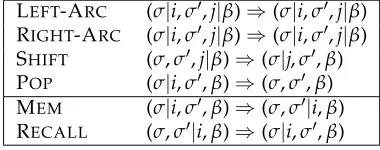
T contains six types of transitions, as shown in Figure 4. We only explain MEM and RECALL:

r

r

LEFT-ARC (σ|i,σ,j|β)⇒(σ|i,σ,j|β) RIGHT-ARC (σ|i,σ,j|β)⇒(σ|i,σ,j|β) SHIFT (σ,σ,j|β)⇒(σ|j,σ,β) POP (σ|i,σ,β)⇒(σ,σ,β) MEM (σ|i,σ,β)⇒(σ,σ|i,β) RECALL (σ,σ|i,β)⇒(σ|i,σ,β)

Figure 4

2.4.2 Theoretical Analysis.The soundness of this system is trivial, and the completeness is also straightforward after we give the construction of an oracle transition sequence for an arbitrary graph. The oracle is computed as follows on thei-th step: We dola,ra, andpoptransitions just like in Section 2.3.2. After that, letbbe the front ofβci−1, we see

if there isj∈σci−1 orj∈σci−1 linked to bby an arc in ¯Aci−1. Ifj∈σci−1, then we do a

sequence ofmemto makejthe top of σci−1; ifj∈σ

ci−1, then we do a sequence ofrcto

makejthe top ofσci−1. When no node inσci−1orσci−1is linked tob, we dosh.

Theorem 2

S2Sis complete with respect to directed graphs without self-loop.

Proof

The completeness immediately follows the fact that the computed oracle sequence is finite, and every time a node is shifted ontoσci, no arc in ¯Aci links nodes inσci to the

shifted node.

2.4.3 Related Systems.G ´omez-Rodr´ıguez and Nivre (2010, 2013) introduced a two-stack– based transition system for tree parsing. Their study is motivated by the observation that the majority of dependency trees in various treebanks are actually planar or two-planar graphs. Accordingly, their algorithm is specially designed to handle projective trees and two-planar trees, but not all graphs. Because many more crossing arcs exist in deep dependency structures and more sentences are assigned with neither planar nor two-planar graphs, their strategy of utilizing two stacks is not suitable for the deep dependency parsing problem. Different from their system, our new system maximizes the utility of two memory modules and is able to handle any directed graphs.

The list-based systems, such as the basic one introduced by Nivre (2008) and the extended one introduced by Choi and Palmer (2011), also use two memory modules. The function of the secondary memory module of their systems and ours is very different. In our design, only nodes involved in a subgraph that contains crossing arcs may be put into the second stack. In the existing list-based systems, both lists are heavily used, and nodes may be transferred between them many times. The function of the two lists is to simulate one memory module that allows accessing any unit in it.

2.5 Extension

2.5.1 Graphs with Loops.It is easy to extend our system to generate arbitrary directed graphs by adding a new transition:

r

Theorem 3

SSandS2Saugmented with SELF-ARCare complete with respect to directed graphs.

deep grammar is considered to license to representation, node labels are usually called “supertags.” To assign supertags to words, namely, nodes in a dependency graph, we can parameterize the SHIFTtransition with tag labels.

3. Statistical Disambiguation

3.1 Transition Classification

A transition-based parser must decide which transition is appropriate given its parsing environment (i.e., configuration). As with many other data-driven dependency parsers, we use a global linear model for disambiguation. In other words, a discriminative classifier is utilized to approximate the oracle function for a transition systemS that maps a configurationcto a transitiontthat is defined onc. More formally, a transition-based statistical parser tries to find the transition sequence c0,m that maximizes the following score

SCORE(c0,m)= m−1

i=0

SCORE(ci,ti+1) (1)

Following the state-of-the-art discriminative disambiguation technique for data-driven parsing, we define the score function as a linear combination of features defined over a configuration and a transition, as follows:

SCORE(ci,ti+1)=θφ(ci,ti+1) (2)

whereφdefines a vector for each configuration–transition pair andθis the weight vector for linear combination.

Exact calculation of the maximization is extremely hard without any assumption ofφ. Even with a properφfor real-word parsing, exact decoding is still impractical for most practical feature designs. In this article, we follow the recent success of using beam search for approximate decoding. During parsing, the parser keeps track of multiple yet a fixed number of partial outputs to avoid making decisions too early. Training a parser in the discriminative setting corresponds to estimating θ associated with rich features. Previous research on dependency parsing shows that structured perceptron (Collins 2002; Collins and Roark 2004) is one of the strongest learning algorithms. In all experiments, we use the averaged perceptron algorithm with early update to estimate parameters. The whole parser is very similar to the transition-based system introduced in Zhang and Clark (2008, 2011b).

3.2 Transition Combination

LEFT-ARC (σ|i,σ,j|β)⇒(σ|i,σ,j|β) RIGHT-ARC (σ|i,σ,j|β)⇒(σ|i,σ,j|β) SHIFT (σ,σ,j|β)⇒(σ|j,σ,β) POP (σ|i,σ,β)⇒(σ,σ,β) MEM (σ|i,σ,β)⇒(σ,σ|i,β) RECALL (σ,σ|i,β)⇒(σ|i,σ,β) LEFT-ARC-SHIFT (σ|i,σ,j|β)⇒(σ|i|j,σ,β) LEFT-ARC-POP (σ|i,σ,j|β)⇒(σ,σ,j|β) LEFT-ARC-MEM (σ|i,σ,j|β)⇒(σ,σ|i,j|β) LEFT-ARC-RECALL (σ|i,σ|i,j|β)⇒(σ|i|i,σ,j|β) RIGHT-ARC-SHIFT (σ|i,σ,j|β)⇒(σ|i|j,σ,β) RIGHT-ARC-POP (σ|i,σ,j|β)⇒(σ,σ,j|β) RIGHT-ARC-MEM (σ|i,σ,j|β)⇒(σ,σ|i,j|β) RIGHT-ARC-RECALL (σ|i,σ|i,j|β)⇒(σ|i|i,σ,j|β)

Figure 5

Original and combined transitions for the two-stack combined system. Two-cycle is not considered here.

improve the performance of a statistical parser, we combine every pair of two successive transitions starting with ARCand transform the proposed two transition systems into two modified ones. For example, in our two-stack–based system, after combining, we obtain the transitions presented in Figure 5.

The number of edges between any two words could be at most two in real data. If there are two edges between two wordswaandwb, it must bewa→wbandwb→wa. We call these two edges a two-cycle, and call this problem the two-cycle problem. In our combined transitions, a LEFT/RIGHT-ARCtransition should appear before a non-ARC transition. In order to generate two edges between two words, we have two strategies:

A) Add a new type of transitions to each system, which consist of a LEFT-ARC transition, a RIGHT-ARCtransition, and any other non-ARC transition (e.g., LEFT-ARC-RIGHT-ARC-RECALLforS2S).

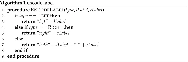
B) Use a non-directional ARCtransition instead of LEFT/RIGHT-ARC. Here, an ARCtransition may add one or two edges depends on its label. In detail, we propose two algorithms, namely, ENCODELABELand DECODELABEL(see Algorithms 1 and 2), to deal with labels for ARCtransition.

Algorithm 1encode label

1: procedureENCODELABEL(type,lLabel,rLabel) 2: iftype==LEFTthen

3: return”left”+lLabel

4: else iftype==RIGHTthen 5: return”right”+rLabel

6: else

7: return”both”+lLabel+”|”+rLabel

Algorithm 2decode combined label, return a pair of left label and right label 1: procedureDECODELABEL(label)

2: iflabel.startswith?(”left”)then 3: return{label[4 :],nil}

4: else iflabel.startswith?(”right”)then 5: return{nil,label[5 :]}

6: else

7: return{label[4 :label.index(|)],label[(label.index(|)+1) :]} 8: end if

9: end procedure

To our best efforts, the strategy B performs better.

First, let us consider accuracy. Generally speaking, it is harder for transition clas-sification if more target transitions are defined. Using strategy A, we should add ad-ditional transitions to handle the two-cycle condition. Based on our experiments, the performance decreases when using more transitions.

Considering efficiency, we can save time by only using labels that appear in training data in strategy B. If we have a total of K possible labels in training data, they will generateK2 _{two-cycle types, but onlykpossible combinations of two-cycle appear in}

training data (k K2_{). In strategy A, we must addK}2_{transitions to deal with all possible}

two-cycle types, but most of them do not make sense. Using fewer two-cycle types helps us eliminate the invalid calculation and save time effectively.

Using strategy B, we change the original edges’ labels and use the ARC(label)–non-ARCtransition instead of LEFT/RIGHT-ARC(label)–non-ARC. An ARC(label)–non-ARC transition should execute the ARC(label) transition first, then execute the non-ARC transition. ARC(label) generates one or two edges depends on its label. Not only do we encode two-cycle labels, but also LEFT/RIGHT-ARC labels. In practice, we only use those labels that appear in training data. Because labels that do not appear only contribute non-negative weights while training, we can eliminate them without any performance loss.

For each transition system and each dependency graph, we generate an oracle transition, and train our model according to this oracle. The constructive proofs pre-sented in Section 2.3 and 2.4 define two kinds of oracles. However, they are not directly applicable when the transition combination strategy is utilized. The main challenge is the existence of cycles. In this article, we propose three algorithms to derive oracles for THMM,SS, andS2S, respectively. Algorithms 3 to 5 illustrate the key steps of the procedure of our system, which find the next transitiontgiven a configurationcand gold graph_Ggold=(_Vx,_Agold) for the three systems. When this key procedure, namely, the EXTRACTONEORACLEmethod, is well defined, the entire transition system can be derived as follows:

EXTRACTORACLE(c0,Agold)

1 oracle=∅

2 whilet←EXTRACTONEORACLE(c0,Agold,nil)do

3 oracle.push back=t

4 c0←t(c0)

Algorithm 3Oracle generation for theTHMMsystem 1: procedureEXTRACTONEORACLE(c,_Agold,label)

2: ifc=(σ|i,j|β,A)∧ ¬∃k[kj∧ ∃l[(i,l,k)∈_Agold]]then 3: iflabel=nilthen

4: returnREDUCE

5: else

6: returnARC(label)◦REDUCE 7: end if

8: else ifc=(σ|i,j|β,A)∧ ∃l[(i,l,j)∈_Agold]then 9: _Agold←_Agold−(i,l,j)

10: returnEXTRACTONEORACLE(c,Agold,label)

11: else if c=(σ|i1|i0,j|β,A)∧ ∃k0k1[k0 j∧k1j∧ ∃l0[(i0,l0,k0)∈ Agold]∧ ∃l1[(i1,l1,k1)∈Agold]∧ ¬∃k0[k0<k0∧ ∃l0[(i0,l0,k0)∈Agold]]∧

∃l1[(i1,l1,k1)∈_Agold]]∧k0<k1]∨ ¬∃k1[k1j∧ ∃l1[(i1,l1,k1)∈_Agold]]then 12: iflabel=nilthen

13: returnSWAP

14: else

15: returnARC(label)◦SWAP 16: end if

17: end if

18: ifc=(σ,j|β,A)then 19: iflabel=nilthen 20: returnSHIFT

21: else

22: returnARC(label)◦SHIFT 23: end if

24: end if 25: returnnil

26: end procedure

We want to emphasize that, although the EXTRACTORACLE methods initialize the parameterLABELin EXTRACTONEORACLEas nil, if an arc transition is predicted in the EXTRACTONEORACLEmethod, it will call EXTRACTONEORACLErecursively to return an ARC(label)–non-ARCtransition and assign a value for thatLABEL.

3.3 Feature Design

Developing features has been shown to be crucial to advancing the state-of-the-art in dependency parsing (Koo and Collins 2010; Zhang and Nivre 2011). To build accurate deep dependency parsers, we utilize a large set of features for transition classification.

To conveniently define all features, we use the following notation. In a configuration with stackσand bufferβ, we denote the top two nodes inσbyσ0andσ1, and the front

ofβbyβ0. In a configuration of the two-stack–based system with the second stackσ,

the top element ofσis denoted byσ₀and the front ofβbyβ0. The left-most dependent

of nodenis denoted byn.lc, the right-most one byn.rc. The left-most parent of noden

Algorithm 4Oracle generation for the online re-ordering system 1: procedureEXTRACTONEORACLE(c,_Agold,label)

2: ifc=(σ|i,j|β,A)∧ ¬∃k[kj∧ ∃l[(i,l,k)∈_Agold]]then 3: iflabel=nilthen

4: returnREDUCE

5: else

6: returnARC(label)◦REDUCE 7: end if

8: else ifc=(σ|i,j|β,A)∧ ∃l[(i,l,j)∈_Agold]then 9: _Agold←_Agold−(i,l,j)

10: returnEXTRACTONEORACLE(c,Agold,label)

11: else ifc=(σ|i,j|β,A)∧ ∃i[i<i∧i ∈σ∧ ∃l[(i,l,j)∈_Agold]]then 12: iflabel=nilthen

13: returnSWAP

14: else

15: returnARC(label)◦SWAP 16: end if

17: end if

18: ifc=(σ,j|β,A)then 19: iflabel=nilthen 20: returnSHIFT

21: else

22: returnARC(label)◦SHIFT 23: end if

24: end if 25: returnnil

26: end procedure

of node nbywn,pn, respectively. Our parser derives the so-called path features from dependency trees. The path features collect POS tags or the first letter of POS tags along the tree between two nodes. Given two nodesn1 andn2, we denote the path feature as

path(n1,n2) and the coarse-grained path feature ascpath(n1,n2). The syntactic head of a nodenis denoted asn.h.

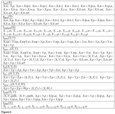
We use the same feature templates for the online re-ordering and the two-stack– based systems, and they are slightly different fromTHMM. Figure 6 defines basic feature template functions. All feature templates are described here.

r

fpair−l(σ0,β0), fpair−l(σ1,β0), fpair(σ0,σ1), ftri(σ0,β0,σ1), ftri−l(σ0,β0,σ0.lp),

ftri−l(σ0,β0,σ0.rp), ftri−l(σ0,β0,σ0.lc), ftri−l(σ0,β0,σ0.lc), ftri−l(σ0,β0,β0.lp),

ftri−l(σ0,β0,β0.lc), ftri−l(σ1,β0,σ1.lp), ftri−l(σ1,β0,σ1.rp), ftri−l(σ1,β0,σ1.lc),

ftri−l(σ1,β0,σ1.lc), ftri−l(σ1,β0,β0.lp), ftri−l(σ1,β0,β0.lc),

fquar−l(σ0,β0,σ0.rp,σ0.rc), fquar−l(σ0,β0,σ0.lc,σ0.lc2),

fquar−l(σ0,β0,σ0.rc,σ0.rc2), fquar−l(σ0,β0,β0.lp,β0.lc),

fquar−l(σ0,β0,β0.lc,β0.lc2), fquar−l(σ1,β0,σ1.rp,σ1.rc),

Algorithm 5Oracle generation for the two-stack–based system 1: procedureEXTRACTONEORACLE(c,_Agold,label)

2: ifc=(σ|i,σs,j|β,A)∧ ¬∃k[kj∧ ∃l[(i,l,k)∈Agold]]then 3: iflabel=nilthen

4: returnREDUCE

5: else

6: returnARC(label)◦REDUCE 7: end if

8: else ifc=(σ|i,σs,j|β,A)∧ ∃l[(i,l,j)∈Agold]then 9: _Agold←_Agold−(i,l,j)

10: returnEXTRACTONEORACLE(c,σs,Agold,label)

11: else ifc=(σ|i,σs,j|β,A)∧ ∃i[i<i∧i ∈σ∧ ∃l[(i,l,j)∈Agold]]then 12: iflabel=nilthen

13: returnMEM

14: else

15: returnARC(label)◦MEM 16: end if

17: else ifc=(σ|i,σs|is,j|β,A)then 18: iflabel=nilthen

19: returnRECALL

20: else

21: returnARC(label)◦RECALL 22: end if

23: end if

24: ifc=(σ,σs,j|β,A)then 25: iflabel=nilthen 26: returnSHIFT

27: else

28: returnARC(label)◦SHIFT 29: end if

30: end if 31: returnnil

32: end procedure

fquar−l(σ1,β0,β0.lp,β0.lc), fquar−l(σ1,β0,β0.lc,β0.lc2), fpath(σ0,β0),

fpath(σ1,β0), fchar(σ0), fchar(β0),

r

uni(β0),

fcontext(σ0), fcontext(β0), fpair−l(σ0,β0), fpair−l(σ1,β0), fpair−l(σ0,β0),

fpair(σ0,σ1), fpair(σ0,σ0), ftri(σ0,β0,σ1), ftri(σ0,β0,σ0), ftri−l(σ0,β0,σ0.lp),

ftri−l(σ0,β0,σ0.rp), ftri−l(σ0,β0,σ0.lc), ftri−l(σ0,β0,σ0.lc), ftri−l(σ0,β0,β0.lp),

ftri−l(σ0,β0,β0.lc), ftri−l(σ1,β0,σ1.lp), ftri−l(σ1,β0,σ1.rp), ftri−l(σ1,β0,σ1.lc),

ftri−l(σ1,β0,σ1.lc), ftri−l(σ1,β0,β0.lp), ftri−l(σ1,β0,β0.lc), ftri−l(σ0,β0,σ0.lp),

ftri−l(σ0,β0,σ0.rp), ftri−l(σ0,β0,σ0.lc), ftri−l(σ0,β0,σ0.lc),

ftri−l(σ0,β0,β0.lp), ftri−l(σ0,β0,β0.lc), fquar−l(σ0,β0,σ0.rp,σ0.rc),

funi(X):

X.w, X.p, X.w◦X.lp.l, X.w◦X.rp.l, X.w◦X.lc.l, X.w◦X.rc.l, X.w◦X.lp.a, X.w◦X.rp.a,

X.w◦X.lc.a, X.w◦X.rc.a, X.w◦X.p.a, X.w◦X.c.a, X.w◦X.lc.set, X.p◦X.lc.set, X.w◦ X.rc.set,X.p◦X.rc.set

g_uni(X):

X.w,X.p,X.w◦X.lp.l,X.p◦X.lp.l,X.w◦X.lc.l,X.p◦X.lc.l,X.w◦X.lp.a,X.p◦X.lp.a,X.w◦ X.lc.a,X.p◦X.lc.a X.w◦X.lc.set,X.p◦X.lc.set

f_context(X):

X₋₂.w, X₋₁.w, X₊₁.w, X₊₂.w, X₋₂.p, X₋₁.p, X₊₁.p, X₊₂.p, X₋₂.w◦X₋₁.w, X₋₁.w◦ X₊₁.w,X₊₁.w◦X₊₂.w,X₋₂.p◦X₋₁.p,X₋₁.p◦X₊₁.p,X₊₁.p◦X₊₂.p

fpair(X,Y):

X.wp◦Y.wp,X.wpY.w,X.wp◦Y.p,X.w◦Y.wp,X.p◦Y.wp,X.w◦Y.w,X.w◦Y.p,X.p◦Y.w,

X.p◦Y.p

f_pair−l(X,Y):

X.wp◦Y.wp, X.wpY.w, X.wp◦Y.p, X.w◦Y.wp, X.p◦Y.wp, X.w◦Y.w, X.w◦Y.p, X.p◦ Y.w, X.p◦Y.p, X.w◦Y.w◦X.rc.a, X.w◦Y.w◦Y.lc.a, X.w◦Y.w◦ X,Y.d, X.p◦Y.p◦ X,Y.d,X.w◦Y.p◦ X,Y.d,X.p◦Y.w◦ X,Y.d,X.p◦Y.p◦X.lc.set,X.p◦Y.p◦X.rc.set,

X.p◦Y.p◦Y.lc.set

ftri(X,Y,Z):

X.w◦Y.p◦Z.p,X.p◦Y.w◦Z.p,X.p◦Y.p◦Z.w,X.p◦Y.p◦Z.p

f_tri−l(X,Y,Z):

X.w◦Y.p◦Z.p◦ X,Z.l, X.p◦Y.w◦Z.p◦ X,Z.l, X.p◦Y.p◦Z.w◦ X,Z.l, X.p◦Y.p◦ Z.p◦ X,Z.l

f_quar−l(X,Y,Z,W):

X.p◦Y.p◦Z.p◦W.p◦ X,Z.l◦ X,W.l

fpath(X,Y):

X,Y.path, X,Y.cpath, X.p◦Y.p◦X.tp.w, X.p◦Y.w◦X.tp.p, X.w◦Y.p◦X.tp.p, X.p◦ Y.p◦Y.tp.w,X.p◦Y.w◦Y.tp.p,X.w◦Y.p◦Y.tp.p

fchar(X):

X_[−1,−1].w,X_[−2,−1].w,X_[−3,−1].w,X_[+1,+1].w,X_[+1,+2].w,X_[+1,+3].w

Figure 6

Feature template functions.

fquar−l(σ0,β0,β0.lp,β0.lc), fquar−l(σ0,β0,β0.lc,β0.lc2),

fquar−l(σ1,β0,σ1.rp,σ1.rc), fquar−l(σ1,β0,σ1.lc,σ1.lc2),

fquar−l(σ1,β0,σ1.rc,σ1.rc2), fquar−l(σ1,β0,β0.lp,β0.lc),

fquar−l(σ1,β0,β0.lc,β0.lc2), fquar−l(σ0,β0,σ0.rp,σ0.rc),

fquar−l(σ0,β0,σ0.lc,σ0.lc2), fquar−l(σ0,β0,σ0.rc,σ0.rc2),

fquar−l(σ0,β0,β0.lp,β0.lc), fquar−l(σ0,β0,β0.lc,β0.lc2), fpath(σ0,β0),

fpath(σ1,β0), fpath(σ0,β0), fchar(σ0), fchar(β0)

4. Tree Approximation

(SRL; Surdeanu et al. 2008; Hajiˇc et al. 2009),CCG-grounded functor–argument (Clark, Hockenmaier, and Steedman 2002) analysis, HPSG-grounded predicate–argument analysis (Miyao, Ninomiya, and ichi Tsujii 2004), and reduction ofMRS(Ivanova et al. 2012), syntactic trees can provide very useful features for semantic disambiguation (Punyakanok, Roth, and Yih 2008). Our parser also utilizes apathfeature template (as defined in Section 3.3) to incorporate syntactic information for disambiguation.

In case syntactic tree information is not available, we introduce a tree approximation technique to induce tree backbones from deep dependency graphs. Such tree backbones can be utilized to train a tree parser which providespseudopath features. In particular, we introduce an algorithm to associate every graph with a projective dependency tree, which we call weighted conversion. The tree reflects partial information about the corresponding graph. The key idea underlying this algorithm is to assign heuristic weights to all ordered pairs of words, and then find the tree with maximum weights. That means a tree frame of a given graph is automatically derived as an alternative for syntactic analysis.

We assign weights to all the possible edges (i.e., all pairs of words) and then determine which edges are to be kept by finding the maximum spanning tree. More formally, given a set of nodesV, each possible edge (i,j), wherei,j∈V, is assigned a heuristic weightω(i,j). Among all trees (denoted asT) overV, the maximum spanning treeTmaxcontains the maximum sum of values of edges:

Tmax=arg max

(V,AT)∈T

(i,j)∈AT

t(i,j)ω(i,j) (3)

We separate theω(i,j) into three parts (ω(i,j)=A(i,j)+B(i,j)+C(i,j)) that are as defined here.

r

r

r

is the length of the given sentence. For dependency parsing, we consider edges with short distance to be more important because those edges can be predicted more accurately in future parsing processes.

r

as possible in original graph, and the direction of the arcs should not be changed if possible. The relationship ofa,b, andcguarantees this.

5. Empirical Evaluation

5.1 Set-up

We present empirical evaluation of different incremental graph spanning algorithms for

CCG-style functor–argument analysis,LFG-style grammatical relation analysis, andHPSG -style semantic dependency analysis for English and Chinese. Linguistically speaking, these types of syntacto-semantic dependencies directly encode information such as coordination, extraction, raising, control, as well as many other long-range dependen-cies. Experiments for a variety of formalisms and languages profile different aspects of transition-based deep dependency parsing models.

Figure 7 visualizes cross-format annotations assigned to the English sentence:A similar technique is almost impossible to apply to other crops, such as cotton, soybeans, and rice. This running example illustrates a range of linguistic phenomena such as coor-dination, verbal chains, argument and modifier prepositional phrases, complex noun phrases, and the so-called tough construction. The first format is from the popular corpus PropBank, which is widely used by various SRL systems. We can clearly see that compared with SRL, SDP uses dense graphs to represent much more syntacto– semantic information. This difference suggests to us that we should explore different algorithms for producing SRL and SDP graphs. Another thing worth noting is that, for the same phenomenon, annotation schemes may not agree with each other. Take the coordination construction, for example. For more details about the difference among different data sets, please refer to Ivanova et al. (2012).

For CCG analysis, we conduct experiments on English and Chinese CCGBank (Hockenmaier and Steedman 2007; Tse and Curran 2010). Following previous experi-mental set-up for EnglishCCGparsing, we use Section 02-21 as training data, Section 00 as the development data, and Section 23 for testing. To conduct Chinese parsing exper-iments, we use data settingCof Tse and Curran (2012). For grammatical relation analy-sis, we conduct experiments on Chinese GRBank data (Sun et al. 2014). The selection for training, development, and test data is also according to Sun et al.’s (2014) experiments. We also evaluate all parsing models using moreHPSG-grounded semantics-oriented data, namely, DeepBank2_{(Flickinger, Zhang, and Kordoni 2012) and EnjuBank (Miyao,}

Ninomiya, and ichi Tsujii 2004). Different from Penn Treebank–converted corpus, DeepBank’s annotations are essentially based on the parsing results given a large-scale linguistically preciseHPSGgrammar, namely, LingGO English resource grammar (ERG; Flickinger 2000), and manually disambiguated. As part of the fullHPSGsign, the ERG also makes available a logical-form representation of propositional semantics, in the framework of minimal recursion semantics (MRS; Copestake et al. 2005). Such seman-tic information is reduced into variable-free bilexical dependency graphs (Oepen and Lønning 2006; Ivanova et al. 2012). In summary, DeepBank gives thereduction of logical-form meaning representations with respect to MRS. EnjuBank (Miyao, Ninomiya, and ichi Tsujii 2004) provides another corpus for semantic dependency parsing. This type of annotation is somehow shallower than DeepBank, given that only basic predicate– argument structures are concerned. Different from DeepBank but similar to CCGBank and GRBank, EnjuBank is semi-automatically converted from Penn Treebank–style an-notations with linguistic heuristics. To conduct HPSGexperiments, we use Sections 00 to 19 as training data and Section 20 as development data to tune parameters. For final

A similar technique is almost impossible to apply to other crops, such as cotton, soybeans and rice

A1

A2

(a) Format 1: Propositional semantics, from PropBank.

A similar technique is almost impossible to apply to other crops, such as cotton, soybeans and rice.

ROOT

BV

arg1 _arg1 arg1 arg1 arg2

arg3

arg1

arg2 implicit conj and c

(b) Format 2:MRS-derived dependencies, from DeepBankHPSGannotations.

A similar technique is almost impossible to apply to other crops , such as cotton , soybeans and rice

ROOT

arg1

arg1 _arg1 arg2arg1 arg1

arg2 arg2 arg1

arg1 arg2arg1 arg1 arg1 arg1

arg2 arg1 arg2 arg1

arg2

(c) Format 3: Predicate-argument structures, from EnjuHPSGannotation.

A similar technique is almost impossible to apply to other crops , such as cotton , soybeans and rice

ROOT

arg1

arg1 _arg1 arg2arg2 arg1

arg2 _arg2 arg3

arg2 arg1arg1 _arg2 arg1

arg2 arg2

arg2

(d) Format 4: Functor-argument structures, from CCGBank. Figure 7

Dependency representations in (a) PropBank, (b) DeepBank, (c) Enju HPSGBank, and (d) CCGBank formats.

evaluation, we use Sections 00 to 20 as training data and section 21 as test data. The DeepBank and EnjuBank data sets are from SemEval 2014 Task 8 (Oepen et al. 2014), and the data splitting policy follows the shared task. Table 1 gives a summary of the data sets for experiments.

Experiments for English CCG-grounded analysis were performed using automat-ically assigned POS-tags that are generated by a symbol-refined generative HMM tagger3 _{(SR-HMM; Huang, Harper, and Petrov 2010). Experiments for English HPSG}

-grounded analysis used POS-tags provided by the shared task. For the experiments on Chinese CCGBank and GRBank, we use gold-standard POS tags.

We use the averaged perceptron algorithm with early update to estimate param-eters, and beam search for decoding. We set the beam size to 16 and the number of iterations to 20 for all experiments. The measure for comparing two dependency graphs is precision and recall of tokens that are defined aswh,wd,ltuples, wherewhis the head,wd is the dependent, and lis the relation. Labeled precision/recall (LP/LR) is the ratio of tuples correctly identified by the automatic generator, and unlabeled precision/recall (UP/UR) is the ratio regardless of l. F-score is a harmonic mean of precision and recall. These measures correspond to attachment scores (LAS/UAS) in de-pendency tree parsing and also used by the SemEval 2014 Task 8. The de facto standard

Table 1

Data sets for experiments. Columns “Training” and “Test” present the number of sentences in training and test sets, respectively.

Language Formalism Data Training Test

English CCG CCGBank 39,604 2,407

HPSG DeepBank 34,003 1,348

HPSG EnjuBank 34,003 1,348

Chinese CCG CCGBank 22,339 2,813

LFG GRBank 22,277 2,557

to evaluateCCGparsers also considers supertags. Because no supertagging is performed in our experiments, only the unlabeled precision/recall/F-score is comparable to the results reported in other papers. And the labeled performance reported here only considers the labels assigned to dependency arcs that indicate the argument types. For example, an arc labelarg1denotes that the dependent is the first argument of the head.

5.2 Parsing Efficiency

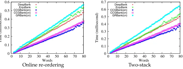
We evaluate the real running time of our final trained parser using realistic data. The test sentences are collected from English Wikipedia and Chinese Gigaword (LDC2005T14). First, we show the influence of beam size in Figure 8. In this experiment, the DeepBank trained models are used for test. We can see that the parsers run in nearly linear time regardless of the beam width in realistic situations. Second, we report the the averaged real running time of models trained on different data sets in Figure 9. Again, we can see that the parser runs in close to linear time for a variety of linguistically motivated representations. The results also suggest that our proposed transition-based parsers can automatically learn the complexity of linguistically motivated dependency structures from an annotated corpus. Note that although within the deep parsing framework, the study of formal grammars is partially relevant for data-driven dependency parsing,

0 0.1 0.2 0.3 0.4 0.5 0.6

0 10 20 30 40 50 60 70 80

Time (millisecond)

Words Beam 2

Beam 4 Beam 8 Beam 16

0 0.1 0.2 0.3 0.4 0.5 0.6

0 10 20 30 40 50 60 70 80

Time (millisecond)

Words Beam 2

Beam 4 Beam 8 Beam 16

Online re-ordering Two-stack

Figure 8

0 0.1 0.2 0.3 0.4 0.5 0.6

0 10 20 30 40 50 60 70 80

Time (millisecond)

Words DeepBank

EnjuBank CCGBank(en) CCGBank(cn) GRBank(cn)

0 0.1 0.2 0.3 0.4 0.5 0.6 0.7

0 10 20 30 40 50 60 70 80

Time (millisecond)

Words DeepBank

EnjuBank CCGBank(en) CCGBank(cn) GRBank(cn)

Online re-ordering Two-stack

Figure 9

Real running time relative to models trained on different data sets.

where our parsers rely on inductive inference from treebank data, and onlyimplicitly

use a grammar.

5.3 Importance of Transition Combination

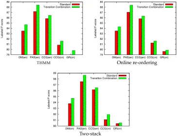
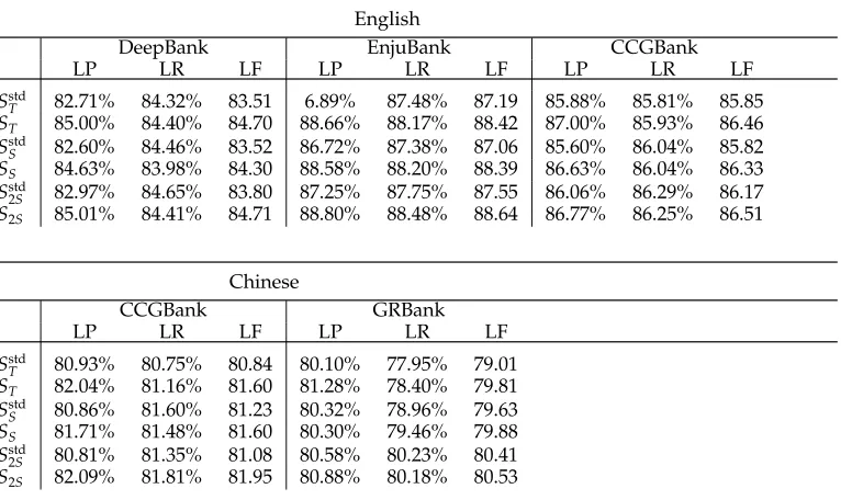
Figure 10 and Table 2 summarize the labeled parsing results on all of the five data sets. In this experiment, we distinguish parsing models with and without transition combination. All models take only the surface word form and POS tag information and do not derive features from any syntactic analysis. The importance of transition combi-nation is highlighted by the comparative evaluation on parsers using this mechanism or not. Significant improvements are observed over a wide range of conditions: Parsers based on different transition systems for different languages and different formalisms almost always benefit. This result suggests a necessary strategy for designing transition systems for producing deep dependency graphs: Configurations should be essentially modified by every transition.

Because of the importance of transition combination, all the following experiments utilize the transition combination strategy.

5.4 Model Diversity and Parser Ensemble

5.4.1 Model Diversity.For model ensemble, besides the accuracy of each single model, it is also essential that the models to be integrated should be very different. We argue that heterogeneous parsing models can be built by varying the underlying transition systems. By reversing the sentence from right to left, we can build other model variants with the same transition system. To evaluate the differences between two modelsAand

B, we define the following metric:

2∗ |DA∩DB| |DA|+|DB|

79 80 81 82 83 84 85 86 87 88 89

DM(en) PAS(en) CCG(en) CCG(cn) GR(cn)

Labeled F-score

Standard Transition Combination

79 80 81 82 83 84 85 86 87 88 89

DM(en) PAS(en) CCG(en) CCG(cn) GR(cn)

Labeled F-score

Standard Transition Combination

THMM Online re-ordering

80 81 82 83 84 85 86 87 88 89

DM(en) PAS(en) CCG(en) CCG(cn) GR(cn)

Labeled F-score

Standard Transition Combination

Two-stack Figure 10

Labeled parsing F-scores of different transition system with and without transition combination. “Standard” denotes thestandardsystems, which do not combine an ARCtransition with its following transition.

5.4.2 Parser Ensemble. Parser ensemble has been shown very effective to boost the performance of data-driven tree parsers (Nivre and McDonald 2008; Surdeanu and Manning 2010; Sun and Wan 2013). Empirically, the two proposed systems together with the existing THMM system exhibit complementary prediction powers, and their combination yields superior accuracy. We present a simple yet effective voting strategy for parser ensemble. For each pair of words in each sentence, we count the number of models that give positive predictions. If the number is greater than a threshold (we set it to half the number of models in this work), we put this arc to the final graph, and label the arc with the most common label of what the models give.

Table 5 presents the parsing accuracy of the combined model where six base models are utilized for voting. We can see that a system ensemble is quite helpful. Given that our graph parsers all run in expected linear time, the combined system also runs very efficiently.

5.5 Impact of Syntactic Parsing

Table 2

Performance of different transition system with and without transition combination on the test set of the DeepBank/EnjuBank data, on the development set of the English and Chinese CCGBank data, and on the development set of the Chinese GRBank data.Sstd

x denotes the

standardsystem, which does not combine an ARCtransition with its following transition.

English

DeepBank EnjuBank CCGBank

LP LR LF LP LR LF LP LR LF

Sstd

T 82.71% 84.32% 83.51 6.89% 87.48% 87.19 85.88% 85.81% 85.85

ST 85.00% 84.40% 84.70 88.66% 88.17% 88.42 87.00% 85.93% 86.46

Sstd

S 82.60% 84.46% 83.52 86.72% 87.38% 87.06 85.60% 86.04% 85.82

SS 84.63% 83.98% 84.30 88.58% 88.20% 88.39 86.63% 86.04% 86.33

Sstd

2S 82.97% 84.65% 83.80 87.25% 87.75% 87.55 86.06% 86.29% 86.17

S2S 85.01% 84.41% 84.71 88.80% 88.48% 88.64 86.77% 86.25% 86.51

Chinese

CCGBank GRBank

LP LR LF LP LR LF

Sstd

T 80.93% 80.75% 80.84 80.10% 77.95% 79.01

ST 82.04% 81.16% 81.60 81.28% 78.40% 79.81

Sstd

S 80.86% 81.60% 81.23 80.32% 78.96% 79.63

SS 81.71% 81.48% 81.60 80.30% 79.46% 79.88

Sstd

2S 80.81% 81.35% 81.08 80.58% 80.23% 80.41

S2S 82.09% 81.81% 81.95 80.88% 80.18% 80.53

(2010) (see Table 6), there is an essential gap between full and shallow parsing-based SRL systems. If we consider a system that takes only word form and POS tags as input, the performance gap will be larger.

When we consider semantics-oriented deep dependency structures, including the representations for CCG-grounded functor–argument (Clark, Hockenmaier, and Steedman 2002) analysis, HPSG-grounded predicate–argument analysis (Miyao, Ninomiya, and ichi Tsujii 2004), and reduction ofMRS(Ivanova et al. 2012), syntactic parses can also provide very useful features for disambiguation. To evaluate the impact of syntactic tree parsing, we include more features, namely, path features, to our parsing models. The detailed description of syntactic features are presented in Section 3.3. In this work, we apply syntactic dependency parsers rather than phrase-structure parsers. Figure 11 summarizes the impact of features derived from syntactic trees. We can clearly see that syntactic features are effective to enhance semantic dependency parsing. These informative features lead to on average 1.14% and 1.03% absolute improvements for English and ChineseCCGparsing. Compared with SRL, the improvement brought by syntactic parsing is smaller. We think one main reason for this difference is the informa-tion density of different types of graphs. SRL graphs usually annotate only on verbal predicates and their nominalization, whereas the semantic graphs grounded byCCGand

Table 3

Model diversity between different models on the test set of the DeepBank/EnjuBank data and on the development set of the English CCGBank data.Srev

x means processing a sentence with systemSxbut in the right-to-left word order.

DeepBank

SS S2S SrevT SrevS Srev2S

ST 0.9285 0.9285 0.8788 0.8796 0.8797

SS 0.9385 0.8748 0.8776 0.8773

S2S 0.8772 0.8802 0.8790

Srev

T 0.9390 0.9364

Srev

S 0.9413

EnjuBank

SS S2S SrevT SrevS Srev2S

ST 0.9504 0.9481 0.9045 0.9038 0.9043

SS 0.9503 0.9046 0.9060 0.9055

S2S 0.9066 0.9087 0.9076

Srev

T 0.9562 0.9565

Srev

S 0.9584

CCGBank

SS S2S SrevT SrevS Srev2S

ST 0.9547 0.9532 0.9155 0.9164 0.9182

SS 0.9575 0.9166 0.9179 0.9187

S2S 0.9200 0.9197 0.9205

Srev

T 0.9586 0.9575

Srev

S 0.9617

Table 4

Model diversity between different models on the development set of the Chinese CCGBank/GRBank data.

CCGBank

SS S2S SrevT SrevS Srev2S

ST 0.9261 0.9262 0.8668 0.8614 0.8658

SS 0.9314 0.8667 0.8593 0.8663

S2S 0.8694 0.8624 0.8683

Srev

T 0.9130 0.9107

Srev

S 0.9230

GRBank

SS S2S SrevT SrevS Srev2S

ST 0.8918 0.8861 0.8398 0.8301 0.8328

SS 0.9058 0.8455 0.8378 0.8414

S2S 0.8460 0.8391 0.8441

Srev

T 0.8969 0.8984

Srev