www.drink-water-eng-sci.net/7/1/2014/
doi:10.5194/dwes-7-1-2014
©Author(s) 2014. CC Attribution 3.0 License.
Drinking Water
Engineering and Science Open Access
Development and evaluation of new behavioral indexes for a biological early warning system using Daphnia
magna
T. Y. Jeong1, J. Jeon2, and S. D. Kim1
1Department of Environmental Science and Engineering, Gwangju Institute of Science and Technology (GIST), 1 Oryong-dong, Buk-gu, Gwangju 500-712, Republic of Korea
2Department of Environmental Chemistry, EAWAG, Swiss Federal Institute of Aquatic Science and Technology, Ueberlandstrasse 133, 8600, Duebendorf, Switzerland
Correspondence to: S. D. Kim ([email protected])
Abstract. New behavioral indexes including combined index (CI), distribution index (DI), toxic index (TI), and altitude index (AI) for a biological early warning system (BEWS) were developed and evaluated using Daphnia magna in this study. The sensitivity and stability of each index were compared to evaluate the per- formance of the indexes through a real-time exposure test with a synthetic copper solution. The applicability of the CI to the field sample was evaluated through an effluent exposure test. The proportional relationship between toxicity level and magnitude of response was much lower in the effluent due to the complexity of water than in the copper solution. The results showed that the CI was most sensitive among the three indexes, while the DI was confirmed as the most useful index among the individual indexes. The combined index (CI) shows not only sensitivity but also stability in normal conditions below the statistically significant threshold (p < 0.01), whereas the individual indexes displayed unstable index values in normal conditions (p > 0.01).
The CI improved performance of the BEWS in terms of sensitivity and stability, and it was confirmed as the higher correlation coefficient between the magnitude of the index and the toxicity level of the water sample.
1 Introduction
Because there is a need for the early detection of water con- tamination in the field of waste water treatment and drink- ing water supply, research has focused on a biological early warning system (BEWS) over the last few decades (Butter- worth et al., 2001; Green et al., 2003). In order to apply the system to regional environmental conditions and achieve dif- ferent monitoring aims, BEWS has been diversified through the employment of various test organisms such as water fleas, mussels, algae, and fish (Baldwin et al., 1994; Benecke et al., 1982; Borcherding et al., 1997; Hendriks et al., 1993).
Among these organisms, Daphnia magna, which is a species of water flea, is widely used because of its usefulness in biomonitoring and high sensitivity to toxic chemicals (van der Schalie et al., 2001). Because of its high sensitivity, be- havioral changes in living Daphnia magna are a powerful real-time indicator in the detection of toxicants in the warn-
ing system. Different types of behavioral parameters have been developed for various kinds of monitoring systems; the monitoring systems of Knie, Kerren Um-welttechnik, and BBE Moldaenke employ swimming activity, phototactic be- havior and swimming speed, and so on (Baillieul et al., 1998;
Kieu et al., 2001). When Daphnia magna faces a change in water quality or a toxic condition in the BEWS, its behav- ior changes markedly, and the level of abnormality is deter- mined from the recorded behavioral data. If the toxic level calculated from the measured data via the specific algorithm increases to above an intentionally fixed threshold, an alarm is triggered by a BEWS (Jeon et al., 2008; Lechlet et al., 2000).
Even if the design of BEWS is appropriate for its goal, the possibility exists that the system will trigger false alarms during its practical operation. Problems can be also caused by uncontrolled variables such as improperly defined thresh- olds or machine error (Butterworth et al., 2001). In addition
to these problems, inherent limitation exists due to behav- ioral deviations in living test organisms during the operation period and between individual organisms. To minimize the possibility of false alarms caused by these biological varia- tions, the simultaneous utilization of a sufficient number of behavioral parameters is needed to supplement the weakness of individual parameters. The Daphnia-Toximeter, produced by BBE Moldaenke, is an example of a system that reduces the frequency of false alarms by simultaneously employing various parameters: velocity, fractal dimension, swimming height, distance between water fleas, and the number of mov- ing water fleas (Baillieul et al., 1998; Michels et al., 1999;
Lechelt et al., 2000).
In a previous study, Jeon et al. (2008) developed a new BEWS, which is equipped with a grid counter device (GC) that identifies the position of the test organism at the grid level instead of at the pixel level. In addition, this system adopted a new algorithm for the alarm function, achieving not only cost effectiveness but also high performance. Ac- cordingly, this study was conducted to enhance the power of the system developed by Jeon et al. The objectives of the present study are as follows: (1) develop a new, reasonable behavioral index that can be applied to a GC device-equipped BEWS; (2) improve the performance of the BEWS by ap- plying various parameters at the same time. To reach these goals, a new type of index called the distribution Index (DI) was developed from newly suggested behavioral parameters, and the altitude Index (AI) was additionally generated by modifying the swimming height parameter of the Daphnia Toximeter (Green et al., 2003; Lechelt et al., 2000). Finally, the combined index (CI) was derived by combining three be- havioral indexes, including the toxic index (TI) that was de- veloped by Jeon et al. The CI performance was evaluated by real-time exposure tests using synthetic water and effluent.
2 Materials and methods
2.1 System design and organism preparation
This study employed a BEWS equipped with a grid counter device. Compositions of the system were the same as in the previous study (Jeon et al., 2008), except that the number of chambers and test organism in each chamber was adjusted from six and one to two and ten, respectively. It can be as- sumed that there were no differences between the TI value from the previous and recent systems except the increase of the statistical power by enlarging total number of the test or- ganism used for the system, because calculation and record- ing method were identical. All methods for culturing Daph- nia magna were conducted according to the USEPA guide- lines (Weber, 1993). A constant temperature of 22.5 ± 1◦C and 16 h of light with 8 h of dark were maintained during the culturing and the exposure test. A synthesized freshwater was prepared within the pH range of 8.0 ± 0.2, with hard- ness of 170 ± 10 mg L−1 and alkalinity of 110 ± 10 mg L−1
as CaCO3 (MgSO4, 9.98 × 10⁻⁴M; CaSO4, 6.98 × 10⁻⁴M;
NaHCO3, 2.28 × 10⁻³M; KCl, 1.07 × 10⁻⁴M).
2.2 Design of indexes 2.2.1 Distribution index
The DI is a newly developed index generated from the swim- ming range parameter. This behavioral parameter is based on the homeostasis of Daphnia’s swimming range. It is well known that the movement of Daphnia is predominantly af- fected by the degree of light intensity and food abundance (Young et al., 1993). Hence, if the food distribution and light intensity are maintained regularly, the swimming range will be consistent. Previous studies of the behavior of Daphnia observed typical changes in activity mass resulting from the stimulus of environmental condition change (Butterworth et al., 2001; Shimizu et al., 2002). This finding motivated our study because activity mass is proportional to movement range. The previous research found that stimulus expressed as avoidance of chemicals or retardation by adverse effects affects the swimming activity, making it greater or lesser than in normal conditions. This means that the movement range could be widened or narrowed, according to the type of be- havior elicited by the stimulus. Additionally, spinning behav- ior, which is an inherent habit of Daphnia in stressful condi- tions (Dodson et al., 1995), could also contribute to dramatic changes in movement ranges. We, therefore, assumed that the range of swimming distribution could be differentiated from normal conditions according to these activity patterns – wide, narrow, and extremely narrow ranges – and developed a new behavioral index based on this assumption.
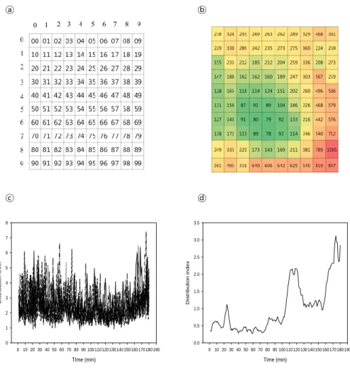
In this study, with the GC device, a rectangular chamber containing water fleas was divided into 100 parts. Each sec- tion was marked for the location of water fleas according to the combination of numbers on the x and y axes; the sec- tions were numbered from 0 to 99 (Fig. 1a). A camera was used to record the spatial data of individual water fleas, and the information was transferred to a computer. When a water flea migrated to another section, a new section number was recorded in the same manner. The data of the locations of the water fleas were shown in detail. The frequencies of ap- pearance at each section were obtained at one minute inter- vals (Fig. 1b), and the distribution level (DL) was calculated (Fig. 1c). If the distribution range of the water fleas was con- centrated in a specific, narrow region of the chambers, only a few sections showed a high frequency of appearance, so the value of DL increased. On the other hand, if each section showed a similar frequency of appearance, it implied that the water fleas moved in a wide range around the test chamber, and the value of DL decreased.
The equation for the DL is DL=σDis
µDis, (1)
ⓐ ⓑ
ⓒ ⓓ
TIme (min)
0 10 20 30 40 50 60 70 80 90 100 110 120 130 140 150 160 170 180 190
Distribution level
0 1 2 3 4 5 6 7 8
Time (min)
0 10 20 30 40 50 60 70 80 90 100 110 120 130 140 150 160 170 180 190
Distribution index
0.0 0.5 1.0 1.5 2.0 2.5 3.0 3.5
Figure 1.Procedure for generating the distribution index. (a) Numbering sections 00 to 99 for recognition of each section. (b) Calculation of appearance frequency of Daphnia magna at each section; this image was colored to easily view the frequency level of occupation. (Red:
highest, Yellow: medium, Green: lowest). (c) Plots of 10 distribution levels derived from 10 Daphnia magna. (d) A Plot of a DI derived from 10 distribution levels.
where σDisis the standard deviation of every observed ap- pearance frequency for 1 min, and µDisis the average of ev- ery observed appearance frequency for 1 min. After this pro- cess, the deviation ratio (Za) for DL was calculated to de- tect whether a considerable change of DL had occurred. The equation for the Za calculation is
Za=Xi−µi si
, (2)
where Xi is the observed DL at the time (i), µi is the aver- age accumulated DL until the time (i), and siis the standard deviation of the accumulated DL until time (i). In terms of statistics, to determine whether a significant difference was observed, a student’s t test was conducted between Za cal- culations in unexposed and exposed periods to the toxicant.
The p values derived from the student’s t test were then trans- formed to the logarithmic value as a log (1/p), and the mov- ing average of the log (1/p) for 5 min was simultaneously calculated. The function of this moving average was to re-
duce the noise in the time series data. Finally, the DI value was calculated from the chamber as shown in Fig. 1d.
2.2.2 Altitude index
The AI is another index based on the swimming height pa- rameter of the Daphnia Toximeter (Lechelt et al., 2000). The concept of swimming height refers to the average swimming position of Daphnia in terms of swimming altitude. Daphnia usually maintain a specific swimming altitude in normal con- ditions because they prefer to swim in an appropriate light range where they cannot be detected by predators (Young et al., 1993). When they are exposed to a toxic condition, this habit is broken. Consequently, when the toxicant stimulates Daphnia, the average swimming position moves to an abnor- mal height, which makes the AI differ from normal condi- tions.
We generated the AI using a grid counter device. As men- tioned in the case of the DI, each chamber was divided into
ⓐ ⓑ
Figure 2.Recognition of swimming altitude of Daphnia magna. (a) Numbering sections 0 to 9 for recognition of each altitude. (b) Example of altitude recognition; the average altitudes of Daphnia magna colored red and blue are calculated.
100 parts, and each section was numbered. The altitude of Daphnia magna was thus recognized according to section numbers from 0 to 9 along the y axis from the top to the bottom, as shown in Fig. 2a. The method used to record the altitude was the same as the method used with DI. The aver- age altitude, called altitude level (AL), was calculated from the recorded altitudes (Fig. 2b). The equation for AL is
AL= µAlt (3)
where µAltis the average of every observed altitude for 1 min.
After this AL calculation, the Za for AL and the log (1/p) for Za using a student’s t test were derived in the same way as for DI. Finally, the AI was produced in real time by adding a step to reduce noise at an interval of 1 min.
2.2.3 Toxic index and combined index
The TI previously developed by Jeon et al. (2008) was also employed in this study for the derivation of the CI and the comparison with the new indexes. All calculation methods were identical to those in that previous study except for the transformation procedure. The raw data on swimming dis- tance were directly used to calculate Za in this study. First, the number of events counted (NC) was measured to indi- cate the swimming distance of Daphnia for 1 min, and the deviation ratio (Za) for NC was calculated to detect whether a considerable change in NC had occurred. Za were com- pared between the normal condition and the toxic condition using a student’s t test, and the log (1/P) was derived. The TI was then calculated with a moving average using the same methods as used for the DI and AI at 1 min intervals. Finally, three parameters were combined into the CI by averaging the values of DI, AI, and TI. This CI was derived every 1 min
and was compared to the DI, AI, and TI through a real-time exposure test.
2.3 Experiment methods 2.3.1 Preparation for tests
The experiment was composed of two different real-time ex- posure tests. The copper exposure test was conducted on synthetic water samples, and the effluent exposure test used effluents sampled from three separate regions. The perfor- mance of the indexes was compared, and the applicability of the CI, which combined three indexes, to the field sam- ple was evaluated using the results of the copper and effluent exposure tests. The age of Daphnia magna used in the tests ranged from 96 h to 120 h for the investigation of behavioral changes. If the test organism is too young, it could be ex- cessively sensitive, or it could die soon after exposure to a toxic chemical. The test organisms were selected from one stock culture to reduce variance in the behavioral character among individuals and the third brood neonates were used.
Every test was conducted without food; the absence of food does not affect the behavior of Daphnia magna (Demeester, 1992).
In the copper exposure test, copper (CuSO4 q5H2O) was used as the representative toxic chemical because of Daph- nia magna’s high sensitivity to it and its wide use in vari- ous industries. Notably, South Korea uses 400 Gg Cu yr−1of copper annually and is the third highest copper-producing country in Asia, making copper an important toxicant and thus relevant for use in this study (Graedel et al., 2004). Be- fore the test, a preliminary acute toxicity test for determin- ing LC50 of copper was conducted over 24 h using Daphnia magna in a static condition. Because 24 h LC50 is typically
chosen as the toxic level of one toxic unit (TU), the determi- nation of a middle concentration of 75 ppb for the main test was based on the 24 h LC50 value of the pre-test (54.371 to 70.717 ppb). The minimum concentration of 18.75 ppb was determined as the basis for the lowest observed effect con- centration (12.5 ppb) in the pre-test to investigate the effects at different concentrations both above and below 24 h LC50.
In the main test, we prepared copper solution daily with hard water at concentrations of 0ppb, 18.75 ppb, 37.5 ppb, 75 ppb, 150 ppb, and 300 ppb. These concentrations are relevant for the BEWS study; it was reported that copper was present in a range of 0.2–11 ppb in the Yeongsan River in South Korea (Kim et al., 2011). The copper exposure tests were triplicated for every test set.
The effluent exposure test sampled three different effluents from waste water treatment plant in Iksan, Yesan, and Yeosu.
The effluent from Yesan was treated with extended aeration process and the effluents from Iksan and Yeosu were treated with conventional activated sludge process. The parameters estimated at the point of exposure study were descripted in Table 1 in the Supplement. The toxicity level of each effluent was respectively confirmed as 0 TU, 50.50 TU, and 1.23 TU by the preliminary 24 h whole effluent toxicity test. The non- toxic effluent from Iksan was used for demonstrating the sta- bility of parameters. Others, including the diluted samples, were used to estimate the early warning capability of param- eters in the field water samples. The effluent from Yesan was diluted to 0.3, 0.7, 1, 1.6, 2.6, 3.3, 3.4, and 4.3 TU. The main contaminants in the sample waters from Yesan and Yeosu were not revealed; however, the characteristics of the two wa- ter samples were quite different. The sample from Yesan was of fresh water and that from Yeosu was of salt water (Kim et al., 2009). The ion concentration estimated by Kim et al. was shown in Table 2 in the Supplement. For the effluent, every exposure test was not replicated to simulate real spillage in- cident in the area of receiving water and water supply source.
2.3.2 Test procedures
The exposure test was conducted for 180 min. Before the ex- posure, we carried out a 120 min feeding time, 180 min adap- tation time, and 180 min unexposed period. During the feed- ing time, we fed Daphnia magna a mixture of Pseudokirch- neriella subcapitata and yeast, CEROPHYLL, and trout chow (YCT). Because the copper exposure test was conducted in the absence of food, Daphnia magna needed a full feeding.
To avoid the effect of environmental conditions such as light, temperature, and food level, we did not support any nutritive element and maintained constant light and temperature con- ditions in the isolated monitoring room after feeding (Dod- son, 1989). In the next step, the adaptation time, Daphnia magna were transferred into two test chambers; each cham- ber contained 10 Daphnia magna. Daphnia magna were al- lowed to swim in the chamber with water flux for 180 min, because an adaption period of at least 2 h is required for
Daphnia magna to obtain a constant swimming pattern by acclimating to water flow after being transferred (Wolf et al., 1998; Untersteiner et al., 2003). In the subsequent step, the unexposed period, the behaviors of Daphnia were recorded for 180 min. These data were used as a control when the stu- dent’s t test was conducted with the data on the exposed pe- riod. In the last step, the exposure period, the influent sample to chambers was replaced with a copper solution or effluent, and this condition was maintained for 180 min. Every pump was stopped during the replacement period. Data obtained for 30 min before and after stopping the pump was excluded to avoid exceptional behavioral changes caused by this pro- cedure. Because the detection time of toxicant exposure by BEWS is not lengthy, we limited the maximum exposure time to 180 min to evaluate whether our system could detect differences in behavior in the early phase of contamination.
2.4 Data analysis
A student’s t test was utilized to compare differences be- tween the behavioral index data during the unexposed and exposed periods. Matlab R2009b, Microsoft Excel 2010, and Sigmaplot 10.0 were used for every data treatment intro- duced in the above sections, including the student’s t test and graph illustration.
3 Results and discussion
3.1 Copper exposure test
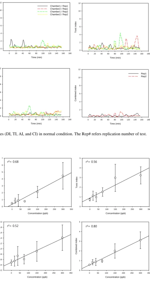
The results of the indexes in the normal condition (0 ppb of copper) are expressed as graphs in Fig. 3. All individual in- dexes (DI, AI, and TI) displayed statistically significant dif- ferences in index values (p < 0.01, index> 2) in the uncon- taminated condition. In contrast, the result of the CI was sta- ble at below 2, a threshold implying a probability of 0.01 % for significant behavioral difference. This result proves the usefulness of combining indexes at the same time in terms of data stability. The raw data from the copper exposure test are summarized in Fig. S1 in the Supplement. Although fluctu- ations in the time series data are apparent, all indexes show the increasing tendency with increased concentration. For the quantitative evaluation of the power of the indexes to reflect changes in toxicity levels, the averages of every calculated index value during exposure time at each concentration were derived as a representative value. Then, linear regressions be- tween the copper concentration and the average values were conducted, as shown in Fig. 4. A comparison of the correla- tion coefficients (r2) showed that the CI had the highest one and the DI showed the highest value among the individual indexes. This result means that the CI is most capable of per- forming accurate early water contamination warning, and the DI best reflects the differences in toxicity levels among the individual indexes derived from the three different behavioral parameters.
Time (min)
0 20 40 60 80 100 120 140 160 180
Distribution index
0 2 4 6 8 10 12
Chamber1 / Rep1 Chamber2 / Rep1 Chamber1 / Rep2 Chamber2 / Rep2
Time (min)
0 20 40 60 80 100 120 140 160 180
Toxic index
0 2 4 6 8 10 12
Time (min)
0 20 40 60 80 100 120 140 160 180
Altitude index
0 2 4 6 8 10 12
Time (min)
0 20 40 60 80 100 120 140 160 180
Combined index
2 4 6 8 10 12
Rep1 Rep2
Figure 3.Results of indexes (DI, TI, AI, and CI) in normal condition. The Rep# refers replication number of test.
Concentration (ppb)
0 50 100 150 200 250 300 350
Distribution index
0 1 2 3 4 5 6 7
Concentration (ppb)
0 50 100 150 200 250 300 350
Toxic index
0 1 2 3 4 5
Concentration (ppb)
0 50 100 150 200 250 300 350
Altitude index
0.2 0.4 0.6 0.8 1.0 1.2 1.4 1.6 1.8 2.0
Concentration (ppb)
0 50 100 150 200 250 300 350
Combined index
0 1 2 3 4 5
r²= 0.56 r²= 0.68
r²= 0.52 r²= 0.80
Figure 4.Linear regressions between representing value (average) of index and copper concentration. The line is regression line and r2is correlation coefficient value.
ⓐ ⓑ
Time (min)
0 20 40 60 80 100 120 140 160 180
Combined index
0 2 4 6 8 10 12
Rep1 Rep2
Toxic unit
0 1 2 3 4 5
Combined index
0 1 2 3 4 5 6
Iksan Yeosu Yesan
Figure 5.(a) Results of Iksan effluent (0TU). Rep# refers replication number. (b) Result of Iksan, Yeosu, and Yesan effluents.
3.2 Effluent exposure test
The results of the CI in the real-time effluent exposure test are expressed as graphs in Fig. 5, where (a) and (b) display the results of the non-toxic effluent from Iksan and differ- ent effluents, respectively. The exposure to non-toxic effluent shows stable index values during the test period at below 2 (p > 0.01, index< 2), which proves the stability of the CI.
In (b), which shows the results of tests using effluent from Yeosu and Yesan, the CI and the TU are not correlated with a huge deviation. This result was expected from the devia- tion of data from the copper exposure test. These fluctuat- ing data confirmed that the system is insufficiently powerful to detect precise toxicity levels of the field samples without replication. The raw data from the effluent exposure tests are summarized in Fig. S2 in the Supplement. This result shows that data from the Yeosu effluent have a higher index value than even the water sample containing a higher number of toxic units, which implies that the different characteristics of water samples can affect the magnitude of index values.
3.3 Discussion
In this study, we suggested a new concept of behavioral pa- rameters related to changes in swimming range. Using this new parameter, the DI and CI were derived, and the utility of combining indexes and the value of the DI for generat- ing the CI were confirmed. The DI showed the best corre- lation between the magnitude of the index and the toxicity level of the water sample among all individual indexes de- rived from three different behavioral parameters. The results showed that the swimming range parameter is a novel indi- cator in terms of both sensitivity and stability. The perfor- mance of the DI was better than that of TI, which is based on the velocity parameter, the best behavioral parameter for monitoring water quality among various parameters (Watson et al., 2007). In addition, the CI was more stable in the nor- mal condition and more sensitive to toxicity change than the
individual indexes were. Because no CI data from the non- toxic water exceeded 2 CI, a statistically meaningful thresh- old at p= 0.01; this study shows the possibility of develop- ing a powerful index that can indicate whether a water sam- ple is contaminated without an intentionally fixed threshold.
Although the CI failed to reflect toxicity levels successfully according to the differentiated TU of the effluent samples without replication of the exposure test, the contribution of this study was in upgrading system stability and sensitivity, which showed the potential to improve BEWSs. Since false alarms are still a major obstacle for accurate BEWSs, this achievement is important in the field.
It is clear that the performance of the BEWS was improved by adopting a new type of behavioral parameter; however, problems in the BEWS occurred. The two major problems were (a) the great deviation in time series data at the same toxicity level, particularly at the lower concentration, and (b) the impact of different water characteristics on index mag- nitude. Although the problems were complemented by repli- cated exposure tests in the case of the copper test, it is not realistic to apply the system when there is no chance to repli- cate early warnings for water contamination. The first prob- lem should be solved by trials to reduce biological deviation, for example, studies strictly selecting homologous organisms (Keui et al., 2001), developing new behavioral parameters and a hardware system (Gerhardt et al., 1998; Michels et al., 1999; Jeon et al., 2008), and improving the performance of hardware and data treatment methods (Li et al., 2008). Re- garding the second problem, more studies analyzing relation- ships between regional water and the behavior of test organ- isms are required at the monitoring site where the system is set (Soldán., 2011). Additionally, test using synthetic wa- ter with a variety of chemical composition, physico-chemical parameters should also be conducted (Gerhardt et al., 2006;
Green et al., 2003; Ren et al., 2007, 2009).
4 Conclusions
The new behavioral indexes DI and CI that can be utilized for BEWS to detect water contamination in drinking water re- source and receiving water were developed from swimming behavior of Daphnia magna. The conclusions derived from this study are as follows.
1. The DI derived from the new behavioral parameter shows the best performance among the three indexes employed in the copper exposure test.
2. The CI improved performance of the BEWS in terms of sensitivity and stability, and it was confirmed as the higher correlation coefficient between the magnitude of the index and the toxicity level of the water sample.
3. Large deviations in the index data and unexpected changes in behavioral responses to water samples con- taining different characteristics occurred in the present study; therefore, further studies to enhance the accuracy and applicability of BEWSs in the field are needed.
Acknowledgements. This study (2013R1A2A2A03014187) was supported by Mid-career Researcher Program through NRF grant funded by the MEST.
Edited by: I. Worm
References
Baillieul, M. and Scheunders, P.: On-line determination of the ve- locity of simultaneously moving organisms by image analysis for the detection of sublethal toxicity, Water Res., 4, 1027–1034, 1998.
Baldwin, I. G., Harman, M. M. I., and Neville, D. A.: Performance characteristics of a fish monitor for detection of toxic substances, Water Res., 28, 2191–2199, 1994.
Benecke, G., Falke, W., and Schmidt, C.: Use of algal fluorescence for an automated biological monitoring system, Bull. Environ.
Contam. Toxico., 28, 385–395, 1982.
Borcherding, J. and Jantz, B.: Valve movement response of the mus- sel Dreissena polymorpha – the influence of pH and turbidity on the acute toxicity of pentachlorophenol under laboratory and field conditions, Ecotoxicology, 6, 153–165, 1997.
Butterworth, F. M., Gunatilaka, A., and Gonsebatt, M. E. Biomon- itors and biomarkers as indicators of environmental change 2: A handbook, Plenum Publishers, New York, 2001.
Demeester, L.: The phototactic behaviour of male and female Daph- nia magna, Anim. Behav., 43, 696–698, 1992.
Dodson, S. I.: Predator-induced reaction norms, Bioscience, 39, 447–452, 1989.
Dodson, S., Hanazato, T., and Gorski, P. R.: Behavioral responses of Daphnia pulex exposed to carbaryl and Chaoborus kairomone, Environ. Toxicol. Chem., 14, 43–50, 1995.
Gerhardt, A. and Clostermann, M.: A new biomonitor system based on magnetic inductivity for freshwater and marine environments, Environ. Int., 24, 699–701, 1998.
Gerhardt, A., Ingram, M. K., Kang, I. J., and Ulitzur, S.: In situ on- line toxicity biomonitoring in water: recent developments, Envi- ron. Toxicol. Chem., 25, 2263–2271, 2006.
Graedel, T. E., Vanbeers, D., Bertram, M., Fuse, K., Gordon, R.
B., Gritsinin, A., Kapur, A., Klee, R. J., Lifset, R. J., Memon, L., Rechberger, H., Spatari, S., and Vexler, D.: Multilevel cycle of anthropogenic copper, Environ. Sci. Technol., 38, 1242–1252, 2004.
Green, U., Kremer, J. H., Zillmer, M., and Moldaenke, C.: Detection of Chemical threat agents in drinking water by an early warning real-time biomonitor, Environ. Toxicol., 18, 368–374, 2003.
Hendriks, A. J. and Stouten, M. D. A.: Monitoring the response of microcontaminants by dynamic Daphnia magna and Leuciscus idus assays in the Rhine delta: biological early warning as a use- ful supplement, Ecotoxicol. Environ. Saf., 26, 265–279, 1993.
Jeon, J. H., Kim, J. H., Lee, B. C., and Kim, S. D.: Development of a new biomonitoring method to detect the abnormal activity of Daphnia magna using automated grid counter device, Sci. Total Environ., 389, 545–556, 2008.
Kieu, N. D., Michels, E., and Meester, L. D.: Phototactic behavior of Daphnia and the continuous monitoring of water quality: In- terference of fish kairomones and food quality, Environ. Toxicol.
Chem., 5, 1098–1103, 2001.
Kim, S. D., Ra, J. S., Kim, K. T., Kim, J. Y., Park, J. E., Kim, H.
D., and Kim, E. Y.: Identification of ecotoxicity from wastew- ater treatment facilities and investigation of sources of toxicity, Ministry Of Environment, Republic of Korea, 2009.
Kim, S. D., Lee, S. H., Kim, H. Y., Kim, J. Y., Jeong, T. Y., Yoon, S. H., Jung, Y. J., and Jung, D. E.: Monitoring and risk assess- ment of the potentially hazardous chemicals in the Yeongsan and the Seomjin rivers. Yongsan River Environment Research Center, Republic of Korea, 2011.
Lechelt, M., Blohm, W., Kirschneit, B., Pfeiffer, M., Gresens, E., Liley, J., Holz, R., Lüring, C., and Moldaenke, C.: Monitoring of surface water by Ultrasensitive Daphnia Toximeter, Environ.
Toxicol., 15, 390–400, 2000.
Li, Y., Seo, D. H., and Lee, W. D.: New classifier applied to biolog- ical early warning systems for toxicity detection, Applications of Digital Information and Web Technologies, 360–365, 2008.
Michels, E., Leynen, M., Cousyn, C., Meester, L. D., and Ollevier, F.: Phototactic behavior of Daphnia as a tool in the continuous monitoring of water quality: Experiments with a positively pho- totactic Daphnia magna clone, Water Res., 2, 401–408, 1999.
Ren, Z., Zha, J., Ma, M., Wang, Z., and Gerhardt, A.: The early warning of aquatic organophosphorus pesticide contamination by on-line monitoring behavioral changes of Daphnia magna, Environ. Monit. Assess., 134, 373–383, 2007.
Ren, Z., Li, Z., Ma, M., Wang, Z., and Fu, R.: Behavioral responses of Daphnia magna to stresses of chemicals with different toxic characteristics, Bull. Environ. Contam. Toxicol., 82, 310–316, 2009.
Shimizu, N., Ogino, C., Kawanishi, T., and Hayashi, Y.: Fractal analysis of Daphnia motion for acute toxicity bioassay, Environ.
Toxicol., 17, 441–448, 2002.
Soldán, P.: Possible way to substantial improvement of early warn- ing system in the International Odra (Oder) River Basin, Environ.
Monit. Assess., 178, 349–359, 2011.
Untersteiner, H., Kahapka, J., and Kaiser, H.: Behavioural response of the cladoceran Daphnia magna to sublethal copper stress-
validation by image analysis, Aquat. Toxicol., 65, 435–442, 2003.
van der Schalie, W. H., Sheddb, T. R., Knechtgesb, P. L., and Wid- der, M. W.: Using higher organisms in biological early warning systems for real-time toxicity detection, Biosens. Bioelectron., 16, 457–465, 2001.
Watson, S. B., Jüttner, F., and Köster, O.: Daphnia behavioural re- sponses to taste and odour compounds: ecological significance and application as an inline treatment plant monitoring tool, Wa- ter Sci. Technol., 55, 23–31, 2007.
Weber, C. I.: Methods for measuring the acute toxicity of effluents and receiving waters to freshwater and marine organisms, U.S.
Environmental Protection Agency, Cincinnati, 1993.
Wolf, G., Scheundersb, P., and Selens, M.: Evaluation of the swim- ming activity of Daphnia magna by image analysis after admin- istration of sublethal cadmium concentrations, Comp. Biochem.
Physiol., 120, 99–105, 1998.
Young, S. and Watt, P.: Behavioral mechanisms controlling verti- cal migration in Daphnia, American Society of Limnology and Oceanography, 39, 70–79, 1993.