Machine Translation
Iftekhar Naim
GoogleParker Riley
University of Rochester Computer Science Department [email protected]
Daniel Gildea
University of Rochester Computer Science Department [email protected]Orthographic similarities across languages provide a strong signal for unsupervised probabilistic transduction (decipherment) for closely related language pairs. The existing decipherment mod-els, however, are not well suited for exploiting these orthographic similarities. We propose a log-linear model with latent variables that incorporates orthographic similarity features. Maximum likelihood training is computationally expensive for the proposed log-linear model. To address this challenge, we perform approximate inference via Markov chain Monte Carlo sampling and contrastive divergence. Our results show that the proposed log-linear model with contrastive divergence outperforms the existing generative decipherment models by exploiting the ortho-graphic features. The model both scales to large vocabularies and preserves accuracy in low- and no-resource contexts.
1. Introduction
Word-level translation models are typically learned by applying statistical word align-ment algorithms on large-scale bilingual parallel corpora (Brown et al. 1993). Building a parallel corpus, however, is expensive and time-consuming. As a result, parallel data are limited or even unavailable for many language pairs. In the absence of a sufficient amount of parallel data, the accuracy of standard word alignment algorithms drops significantly. This is also true of supervised neural methods: Even with hundreds of thousands of parallel training sentences, neural methods only achieve modest results
Submission received: 9 October 2017; revised version received: 16 March 2018; accepted for publication: 15 May 2018.
(Zoph et al. 2016). Low- and no-resource languages generally do not have parallel cor-pora, and even their monolingual corpora tend to be small. However, these monolingual corpora can often be downloaded from the Internet, and are much easier to obtain or produce than parallel corpora. Leveraging useful information from monolingual cor-pora can be extremely helpful for learning translation models for low- and no-resource language pairs.
Decipherment algorithms (so-called because of the assumption that one language is a cipher for the other) aim to exploit such monolingual corpora in order to learn translation model parameters, when parallel data are limited or unavailable (Koehn and Knight 2000; Ravi and Knight 2011; Dou, Vaswani, and Knight 2014). The key intuition is that similar words andn-grams tend to have similar distributional properties across languages. For example, if a bigram appears frequently in the monolingual source corpus, its translation is likely to appear frequently in the monolingual target corpus, and vice versa. This is especially true when the corpora share similar topics and context. Furthermore, for many such language pairs, we observe similar monotonic word ordering—that is, the translation of a bigram is often the same as the concatenation of the translations of individual unigrams (consider the shared use of postnominal adjectives in the Frenchmaison bleuand Spanishcasa azul). Although this certainly is not always true, we assume that it is common enough to provide a useful signal. The goal of decipherment algorithms is to leverage such statistical similarities across languages, and effectively learn word-level translation probabilities from monolingual data.
Existing decipherment methods are predominantly based on probabilistic genera-tive models (Koehn and Knight 2000; Ravi and Knight 2011; Dou and Knight 2012; Nuhn and Ney 2014). These models primarily focus on the statistical similarities between the n-gram frequencies in the source and the target language, and rely on the expectation maximization (EM) algorithm (Dempster, Laird, and Rubin 1977) or its faster approxi-mations. However, there can be many other types of statistical and linguistic similari-ties across languages beyondn-gram frequencies (similarities in spelling, word-length distribution, syntactic structure, etc.). Unfortunately, existing generative models do not allow incorporating such a wide range of linguistically motivated features. Previous research has shown the effectiveness of incorporating linguistically motivated features for many different unsupervised learning tasks, such as unsupervised part-of-speech in-duction (Haghighi and Klein 2006; Berg-Kirkpatrick et al. 2010), word alignment (Dyer et al. 2011; Ammar, Dyer, and Smith 2014), and grammar induction (Berg-Kirkpatrick et al. 2010).
Many pairs of related languages share vocabulary or grammatical structure due to borrowing or inheritance: the Englishaquaticand Spanishaguashare the Latin root aqua, and the Englishbeigewas borrowed from French. As a result, orthographic fea-tures provide crucial information for determining word-level translations for closely related language pairs. Church (1993) leveraged orthographic similarity for character alignment. Haghighi, Berg-Kirkpatrick, and Klein (2008) proposed a generative model for inducing a bilingual lexicon from monolingual text by exploiting orthographic and contextual similarities among the words in two different languages. The model proposed by Haghighi et al. learns a one-to-one mapping between the words in two languages by analyzing type-level features only, while ignoring the token-leveln-gram frequencies. We propose a decipherment model that unifies the type-level feature-based approach of Haghighi et al. with token-level EM-based approaches such as Koehn and Knight (2000) and Ravi and Knight (2011).
relationship between word frequency and length (Zipf 1949), so the tendency of words and their translations to have similar frequencies (Rapp 1995) may apply to length as well. Our feature-rich log-linear model can easily incorporate such length-based similarity features.
One of the key challenges with the proposed latent variable log-linear model is the high computational complexity of training, as it requires normalizing globally via summing over all possible observations and latent variables. As a result, an exact implementation is impractical even for the moderate vocabulary size of most low-resource languages. To address this challenge, we perform approximate inference using Markov chain Monte Carlo (MCMC) sampling for scalable training of the log-linear decipherment models. We present a series of increasingly scalable approximations, each most suitable for a different amount of available data. They are applicable in contexts ranging from no-resource languages (such as “lost” languages, a context considered by Snyder, Barzilay, and Knight [2010]) to languages with a modest amount of data that is still insufficient for state-of-the-art unsupervised methods based on word embeddings.
The main contributions of this article are as follows.
r
We propose a feature-based decipherment model for low- and no-resource languages that combines both type-level orthographic features and token-level distributional similarities. Our proposed model outperforms the existing EM-based decipherment models.r
We apply three different MCMC sampling strategies for scalable training and compare them in terms of running time and accuracy. Our results show that contrastive divergence (Hinton 2002)–based MCMC sampling can dramatically improve the speed of the training, while achieving comparable accuracy.r
We extend the contrastive divergence method to sample entire sentences, rather than bigram pairs, allowing more context to be used inreconstructing latent translations.
r
Finally, we extend the model to exploit parallel as well as monolingual data, for situations in which limited amounts of parallel data may be available.The remainder of the article is organized as follows. In Section 2, we introduce the general problem formulation for monolingual decipherment, and present our notations. We discuss the background literature on different decipherment models for machine translation in Section 3. Section 4 describes the proposed feature-based decipherment model. A detailed discussion of MCMC sampling–based approximations follows in Section 5. We extend the fully monolingual model to exploit parallel data in Section 6. Our orthographic features are described in Section 7. Finally, we present our detailed results in Section 8 and conclude with our findings and discuss our future work in Section 9.
2. Problem Formulation
Table 1
Our notations and symbols.
Symbol Meaning
NF Number of unique source bigrams
NE Number of unique target bigrams
VF Source vocabulary
VE Target vocabulary
V max(|VF|,|VE|)
N Number of samples
K Beam size for precomputed lists
φ Unigram level feature function
Φ Φ
Φ Bigram level feature function:ΦΦΦ =φ1+φ2
language. Although the sentences in the source and target corpus are independent of each other, there exist distributional and lexical similarities among the words of the two languages. We aim to automatically learn the translation probabilitiesp(f|e) for all source wordsf and target wordseby exploiting the similarities between the bigrams in FandE.
As a simplification step, we break down the sentences in the source and target corpus as a collection of bigrams. Let F contain a collection of source bigrams f1f2, andE contain a collection of target bigramse1e2. Let the source and target vocabulary beVFandVE, respectively. LetNFandNEbe the number of unique bigrams inFandE,
respectively. We assume that the corpusFis an encrypted version of a plaintext in the target language. Each source wordf ∈VFis obtained by substituting one of the words
e∈VEin the plaintext. However, the mappings between the words in the two languages
are unknown, and are learned as latent variables. Table 1 summarizes the notations and symbols used in this article.
3. Background Research
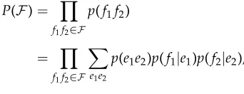
Existing decipherment models assume that each source bigramf1f2inFis generated by first generating a target bigrame1e2 according to the target language model, and then substituting e1 ande2 with f1 and f2, respectively. The generative process is typically modeled via a hidden Markov model (HMM), as shown in Figure 1(a). The target bigram language modelp(e1e2) is trained from the given monolingual target corpusE. The unknown translation probabilitiesp(f|e) are learned by maximizing the likelihood of the observed source corpusF:
P(F)= Y
f1f2∈F
p(f1f2) (1)
= Y
f1f2∈F
X
e1e2
p(e1e2)p(f1|e1)p(f2|e2),
wheree1ande2are the latent variables, indicating the target words inVEcorresponding
a) b)
e1
P(e1) e2
f1 f2
P(e2|e1)
P(f1|e1) P(f2|e2)
e1 e2
f1 f2
P(e1,e2)
[image:5.486.57.429.60.176.2]expwTφ(f1,e1) expwTφ(f2,e2)
Figure 1
The graphical models for the existing directed HMM (a) and the proposed undirected MRF (b).
and several methods have been proposed for maximizing it. In this work, we seek to combine a number of them for improved performance.
3.1 Expectation Maximization (EM)
The expectation maximization (EM) (Dempster, Laird, and Rubin 1977) algorithm has been widely applied for solving the decipherment problem (Knight and Graehl 1998; Knight and Yamada 1999; Koehn and Knight 2000). In the E-step, for each source bigram f1f2, we estimate the expected counts of the latent variablese1ande2 over all the target words inVE. In the M-step, the expected counts are normalized to obtain the translation
probabilitiesp(f|e). The computational complexity of the EM algorithm isO(NFV2) and
the memory complexity isO(V2), whereNFis the number of unique bigrams inFand
V=max(|VF|,|VE|). As a result, the regular EM algorithm does not scale well to large
vocabulary sizes, both in terms of running time and memory.
To address this challenge, Ravi and Knight (2011) proposed the iterative EM algo-rithm, which starts with theKmost frequent words fromF and E and performs EM-based decipherment. Next, the source and target vocabularies are iteratively extended byKnew words, while pruning low-probability entries from the probability table. The computational complexity of each iteration becomesO(NFK2).
3.2 Bayesian Decipherment Using Gibbs Sampling
3.3 Slice Sampling
Each Gibbs sampling operation requires estimating the probability of choosing every target word e∈VE, which requires O(V) operations. To address this issue, Dou and
Knight (2012) proposed a slice sampling approach with precomputed top-K lists for p(e|f) andp(e1e2). Slice sampling involves selecting a thresholdT between 0 and the probability of the current sample, and then uniformly picking a random new sample from all candidates with probability greater than T. Using sorted top-K lists makes this faster than Gibbs sampling on average, although sometimes the top-Klists fail to provide all the candidates, in which case the method has to fall back to sampling from the entire vocabulary, which requiresO(V) operations.
3.4 Beam Search
Nuhn and colleagues (Nuhn, Schamper, and Ney 2013; Nuhn and Ney 2014; Nuhn, Schamper, and Ney 2015) showed that beam search can significantly improve the speed of EM-based decipherment, while providing comparable or even slightly better accuracy. Beam search prunes less-promising latent states by maintaining two constant-sized beams, one for the translation probabilities p(f|e) and one for the target bigram probabilitiesp(e1e2)—reducing the computational complexity toO(NF). Furthermore, it
saves memory because many of the word pairs (f,e) are never considered because they are not in the beam.
3.5 Feature-Based Generative Models
Haghighi, Berg-Kirkpatrick, and Klein (2008) proposed a canonical correlation analysis– based model for automatically learning the mapping between the words in two lan-guages from monolingual corpora only. They used orthographic information (character substring features) and context information (co-occurrence statistics within a window) for their features; we use edit distance as our orthographic information, and we op-erate on bigrams for our context information. Although their model uses an EM-style algorithm, it does not iterate over the corpus data.
Ravi (2013) proposed a Bayesian decipherment model based on hash sampling, which takes advantage of feature-based similarities between source and target words. However, the feature representation was not integrated with their decipherment model, and was only used for efficiently sampling candidate target translations for each source word. Furthermore, the feature-based hash sampling included only contextual features (in the form ofn-gram co-occurrence information), and did not consider orthographic features. In contrast, our log-linear model integrates both type-level orthographic fea-tures and token-level bigram frequencies.
3.6 Embedding-Based Models
translations, but do use document-aligned Wikipedia data, and only consider words appearing at least 1,000 times. Both methods train word embeddings using data sets with millions of words, limiting their applicability to low resource languages, even more so for languages with the small amount of data that we experiment with in this work.
4. Feature-Based Decipherment
Our feature-based decipherment model is based on a chain structured Markov random field (MRF; Figure 1(b)), which jointly models the observed source bigramsf1f2 and corresponding latent target bigrame1e2. For each source wordf ∈VF, we have a latent
variablee∈VEindicating the corresponding target word. The joint probability
distri-bution is:
p(f1f2,e1e2)= Z1
wp(e1e2) expw
TΦΦΦ(f
1f2,e1e2)
whereΦΦΦ(f1f2,e1e2) is the feature function for the given source and the target bigrams,
wis the model parameters, andZwis the normalization term. We assume that the
fea-ture function decomposes into feafea-tures of aligned word pairs (motivated by the obser-vation in Section 1 that word order is generally preserved across bigram translations):
Φ
ΦΦ(f1f2,e1e2)=φ(f1,e1)+φ(f2,e2) (2)
The featuresφ, which will be described in more detail in Section 7, include features for orthographic similarity as well as indicator features φf,e for each word pair. The normalization term is defined as:
Zw= X
f1f2
X
e1e2
p(e1e2) expwTΦΦΦ(f1f2,e1e2)
This gives our model the conditional random field (CRF)–like dependency structure shown in Figure 1. In our model, however, the termp(e1,e2) is estimated from a mono-lingual target corpus, and is held constant when training the weightsw.
We train the model on a monolingual source corpus, treating the target words as latent variables. This gives us a latent variable CRF model (Quattoni, Collins, and Darrell 2004), where the likelihood of our monolingual source corpus is:
L= 1 |F|
X
f1f2∈F logX
e1e2
The gradient of the log-likelihood can be written as the difference of two expectations of feature vectors:
∂L
∂w =
∂ ∂w|F1|
X
f1f2∈F logX
e1e2
p(f1f2,e1e2) (4)
= ∂
∂w|F1| X
f1f2∈F logX
e1e2 1
Zwp(e1e2) expw
TΦΦΦ(f1f2,e1e2) (5)
= 1 |F|
X
f1f2∈F
"
∂ ∂wlog
X
e1e2
p(e1e2) expwTΦΦΦ(f1f2,e1e2)−∂∂wlogZw #
(6)
= 1 |F|
X
f1f2∈F
"
1 Zw(f1f2)
∂ ∂w
X
e1e2
p(e1e2) expwTΦΦΦ(f1f2,e1e2)
#
− ∂
∂wlogZw (7)
= 1 |F|
X
f1f2∈F
"
1 Zw(f1f2)
X
e1e2
Φ
ΦΦ(f1f2,e1e2)p(e1e2) expwTΦΦΦ(f1f2,e1e2)
#
−Zw∂∂wZw
= 1 |F|
X
f1f2∈F
" X
e1e2
Φ Φ
Φ(f1f2,e1e2)p(f1f2|e1e2)
# − 1 Zw ∂ ∂w X
f1f2
X
e1e2
p(e1e2) expwTΦΦΦ(f1f2,e1e2)
= 1 |F|
X
f1f2∈F
Ee1e2|f1f2
ΦΦΦ(f1f2,e1e2)
− 1
Zw X
f1f2
X
e1e2
Φ
ΦΦ(f1f2,e1e2)p(e1e2) expwTΦΦΦ(f1f2,e1e2)
= 1 |F|
X
f1f2∈F
Ee1e2|f1f2
ΦΦΦ(f1f2,e1e2)
−Ef
1f2,e1e2
ΦΦΦ(f1f2,e1e2)
(8)
=EForced−EFull (9)
Here, the first term is the expectation with respect to the empirical data distribution. We refer to it as the “forced expectation,” as the source text is assumed to be given. The second term is the expectation with respect to our model distribution, and referred to as “full expectation.”
4.1 Estimating Forced Expectation (EForcedForcedForced)
We first estimate the forced expectation, which we defined in Equation (8) to be:
EForced= X
f1f2∈F 1 Zw(f1f2)
X
e1e2∈VE2
p(e1e2) expwTΦΦΦ(f1f2,e1e2)
ΦΦΦ(f1f2,e1e2) (10)
whereZ(f1f2) is the normalization term givenf1f2:
Zw(f1f2)=
X
e1e2∈V2E
For each observedf1f2∈F, we sum over all possiblee1e2 ∈V2E, which requiresO(NFV2)
computations.
4.2 Estimating Full Expectation (EFullFullFull)
For the full expectation, we assume that both the source text and latent variables are unknown, resulting in a sum over all the possible source bigramsf1f2, and associated latent variablese1e2:
EFull= Z1
g
X
f1f2∈V2F X
e1e2∈V2E
p(e1e2) expwTΦΦΦ(f1f2,e1e2)
Φ
ΦΦ(f1f2,e1e2)
whereZgis the global normalization term:
Zg=
X
f1f2∈VF2 X
e1e2∈V2E
p(e1e2) expwTΦΦΦ(f1f2,e1e2)
The computational complexity isO(V4).
5. MCMC Sampling for Faster Training
The overall computational complexity of estimating the exact gradient isO(NFV2+V4),
which is impractical even for a modest-sized vocabulary. We apply several MCMC sampling methods to approximate the forced and full expectations. We first propose using Gibbs sampling for both the forced and full expectation terms. We then propose a faster approximation using independent Metropolis Hastings sampling for just the forced expectation term. We then propose an even faster approximation using con-trastive divergence for estimating both terms. We then extend this method to sam-ple at the sentence level rather than at the bigram level, with the goal of increasing accuracy.
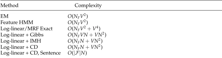
Computation times for the methods presented are summarized in Table 2.
5.1 Gibbs Sampling
[image:9.486.53.435.560.660.2]5.1.1 Gibbs Sampling for Forced Expectation.Rather than summing over all target bigrams e1e2, we approximate the forced expectation by taking N samples of e1e2 for each
Table 2
The worst case computational complexities per iteration for different decipherment algorithms. Note that we observed thatNFtended to scale linearly withV.
Method Complexity
EM O(NFV2)
Feature HMM O(NFV2)
Log-linear/MRF Exact O(NFV2+V4)
Log-linear + Gibbs O(NFVN+VN2)
Log-linear + IMH O(NFN+VN2)
Log-linear + CD O(NFN+VN2)
observedf1f2, and take an average of the features for these samples. For each observed f1f2, the following steps are taken:
r
Start with an initial target bigrame1e2.r
Fixe2and samplee1according to the following probability distribution:P(e1|e2,f1f2)= Z1
gibbs
p(e1e2) expwTΦΦΦ(f1f2,e1e2)
whereZgibbsis the normalization term over all possiblee1in the target vocabulary.
r
Next, fixe1and draw a new samplee2similarly according toP(e2|e1,f1f2), and continue samplinge1ande2alternately untilNsamples are drawn. Drawing each sample requires O(V) operations, as we need to estimate the normal-ization termZgibbs. The computational complexity of estimating the forced expectationbecomes O(NFVN), which is expensive as V can be large (and NF generally scales
withV).
5.1.2 Gibbs Sampling for Full Expectation.To efficiently estimate the full expectation, we sampleNsource bigramsf1f2from our model. The Gibbs sampling procedure is:
r
Start with an initial randomf1f2.r
Fixf2, and sample a newf1according top(f1|f2):p(f1|f2)= 1
Z0gibbs
X
e1
X
e2
p(e1e2) expwTΦΦΦ(f1f2,e1e2)
where
Z0gibbs=X
f1
X
e1
X
e2
p(e1e2) expwTΦΦΦ(f1f2,e1e2)
r
Next fixf1and samplef2according toP(f2|f1). Continue alternating until Nsamples are drawn.The computational complexity of exactly estimatingp(f1|f2) isO(V3), resulting in the computational complexityO(V3N), which is impractical for all but the smallest vocab-ularies. However, rather than summing over all possiblee1e2, we can approximate via sampling. For eachf1f2, we first sampleNsamplese1e2according top(e1e2). LetSbe the set ofNsamples of target bigrams. Next, we approximatep(f1|f2) as
p(f1|f2)= Z 1
approx
X
e1e2∈S
expwTΦΦΦ(f1f2,e1e2)
where Zapprox=Pf1
P
e1e2∈Sexpw
TΦΦΦ(f
5.2 Independent Metropolis Hastings (IMH)
In our experiments, the Gibbs sampling for our log-linear model was still somewhat slow, and will not scale well to larger experimental settings. To address this challenge, we apply IMH sampling, which relies on a proposal distribution and does not require normalization. However, finding an appropriate proposal distribution can sometimes be challenging, as it needs to be close to the true distribution for faster mixing and must be easy to sample from.
For the forced expectation, one possibility is to use the bigram language model p(e1e2) as a proposal distribution. However, the bigram language model did not work well in practice. Becausep(e1e2) does not depend onf1f2, it resulted in slow mixing and exhibited a bias toward highly frequent target words.
Instead, we chose an approximation ofp(e1e2|f1f2) as our proposal distribution. To simplify sampling, we assumee1ande2to be independent of each other for any given f1f2. Therefore, the proposal distributionq(e1e2|f1f2)=qu(e1|f1)qu(e2|f2), wherequ(e|f)
is a probability distribution over target unigrams for a given source unigram. We define qu(e|f) as follows:
qu(e|f)=(1−pb)qs(e|f)+pbV1
wherepbis a small back-off probability with which we fall back to the uniform
distribu-tion over target unigrams. The other termqs(e|f) is a distribution over the target words
efor which the weightwf,eof the word pair featureφf,eis non-zero:
qs(e|f)=
(
1
Zimhexpw
Tφ(f,e), ifw f,e6=0
0, otherwise
Here,Zimhis a normalization term over all theesuch thatwf,e6=0. The weight vectorw
is sparse, as only a small number of translation features (f,e) (Section 7) are observed during sampling. Furthermore, we updateqsonly once every five iterations of gradient
descent.
The actual target distribution is:
p(e1e2|f1f2)∝p(e1e2) expwTΦΦΦ(f1f2,e1e2) (11)
For eachf1f2 ∈F, we take the following steps during sampling:
r
Start with an initial English bigram:he1e2i0.r
Let the current sample behe1e2ii. Next, samplehe1e2ii+1from the proposal distributionq(e1e2|f1f2).
r
Accept the new sample with the probability:Pa=p(
he1e2ii+1|f1f2) p(he1e2ii|f1f2)
q(he1e2ii|f1f2)
The IMH sampling reduces the complexity of the forced expectation estimation to O(NFN),1 which is significantly less than the complexity of O(NFVN) in the case of
Gibbs sampling. However, we could not apply IMH while estimating the full expec-tation, as finding a suitable proposal distribution is more complicated. Therefore, the overall complexity remains:O(NFN+VN2).
5.3 Contrastive Divergence-Based Sampling
The main reason for the slow training of the proposed log-linear MRF model is the high computational cost of estimating the partition function Zg when estimating the
full expectation. A similar problem arises while training deep neural networks. An increasingly popular technique to address this issue is to perform contrastive diver-gence (Hinton 2002), which allows us to avoid estimating the partition function.
For each observed source bigramf1f2 ∈F, contrastive divergence sampling works as follows:
r
Sample a target bigrame1e2according to the distributionp(e1e2|f1f2). We perform this step using IMH, as discussed in the previous section.r
Sample a reconstructed source bigramhf1f2ireconby sampling from thedistributionp(f1f2|e1e2), again via IMH.
We take n such samples of e1e2 and corresponding hf1f2irecon. For each sample and reconstruction pair, we update the weight vector by an approximation of the gradient:
∂L
∂w ≈ΦΦΦ(hf1f2i
data,e1e2)−ΦΦΦ(hf1f2irecon,e1e2)
5.4 Sentence-Level Sampling
Up to this point, we have considered parallel source/target bigram pairs in isolation, but it may be helpful to take larger contexts into account in decipherment. In this section, we extend the sampling procedures to resample an entire source/target sen-tence pair at each iteration. Although our features are functions of individual bigrams, sentence-level sampling gives us the benefit of looking at an individual word’s left and right context when considering alternative translations. More generally, the HMM-like feature structure also allows information to flow through the entire sentence from beginning to end.
Mathematically, we assume, as we did in the bigram case, that our features can be written as a functionφ(f,e) of a pair of French and English words. We use the notation
ΦΦΦ(f,e)=
|f|
X
i=0
φ(fi,ei)
to denote the feature vector for an entire sentence pair; we will assume that the French and English sequences have the same length. Analogously to Equation (4), the gradient
of the log-likelihood can be written as the difference between a forced expectation and full expectation, now at the level of sentences rather than bigrams:
∂L
∂w =Ee|f[ΦΦΦ(f,e)]−Ee,f[ΦΦΦ(f,e)] =EForced−EFull
We estimate these two terms with a sentence-level sampling algorithm based on contrastive divergence. At a high level, given an observed French sentence, it samples a hidden English sequence according top(e|f) in order to estimate the forced expectation term of the update, and then samples a French sentence according top(f|e) to estimate the full expectation, as shown in Algorithm 1. However, because the individual English words are not independent, due to the bigram language model, the sampling ofp(e|f) is itself broken down into a sequence of Gibbs sampling steps, sampling one word at a time while holding the others fixed, as shown in Algorithm 2. This process is iterated to produce a total ofNsamples of the English sequence, with each sample initialized with the previous sample (line 4 of Algorithm 1). The entire process is initialized with a Viterbi decoding of the best English sequence under the current parameters (line 2 of Algorithm 1). Empirically, we found that this initialization sped up training by reducing the number of samples necessary.
Algorithm 1Sentence-level contrastive divergence algorithm
1: procedureSENTCONTRASTIVEDIVERGENCE(f)
2: e(0)←VITERBI(f,w)
3: fornin 1,. . .,Ndo
4: (e(n),f(n)) = SAMPLESENTENCEPAIR(e(n−1),f)
5: w←w+ 1
N
P
n ΦΦΦ(f,e(n))−ΦΦΦ(f(n),e(n))
Algorithm 2Sentence-level sampling algorithm procedureSAMPLESENTENCEPAIR(e,f)
fori←1,. . .,|f|do
ei∼ Z1p(ei−1ei)p(eiei+1) expwTφ(ei,fi)
fori←1,. . .,|f|do
fi∼ Z1 expwTφ(ei,fi)
return(e,f)
6. Exploiting Parallel Data
parallel data may help prevent the decipherment model from aligning words that are spuriously similar “false friends” when analyzing the monolingual data.
Mathematically, we wish to define a single probability model that can apply to both parallel and monolingual data, and choose feature weights w that optimize the total likelihood of the parallel and monolingual data together. Probability models for word alignment of parallel data are one of the original problems studied in statistical machine translation (Brown et al. 1993). We wish to apply our log-linear feature-based model to parallel data, making the problem setting similar to that of Dyer et al. (2011). For simplicity, we assume a bag of words model that does not take into account the order of the words in the English sentence, resulting in a log-linear feature-based version of IBM Model 1.
We implement training for this model by modifying our sentence-level contrastive divergence method described in Section 5.4. We constrain the sampling of the English wordseforcedused to approximate theEForcedterm by allowing only English words that
appear in the English side of the parallel sentence pair. We sample a separate sequence of English wordsefor theEFullterm as before. The algorithm for parallel data is shown
in Algorithm 3, where the English side of the parallel sentence pair is provided as an additional argument ˆe. This set of words is used to constrain the choices of the Viterbi initialization ofeforced(line 2). The observed English sentence ˆeis also used to constrain
the choice of sample in Algorithm 4; the indicator function I(ei∈ ˆe) ensures that any
English words not present inˆehave zero probability of being sampled.
Algorithm 3Constrained contrastive divergence algorithm
1: procedureCONSTRAINEDSENTCONTRASTIVEDIVERGENCE(f,ˆe)
2: e(0)forced←CONSTRAINEDVITERBI(f,w,ˆe)
3: e(0)←VITERBI(f,w)
4: fornin 1,. . .,Ndo
5: e(forcedn) = CONSTRAINEDSAMPLESENTENCE(eforced(n−1),f,ˆe)
6: (e(n),f(n)) = SAMPLESENTENCEPAIR(e(n−1),f)
7: w←w+ 1
N
P
n
Φ
ΦΦ(f,e(forcedn) )−ΦΦΦ(f(n),e(n))
Algorithm 4Constrained sentence-level sampling algorithm
1: procedureCONSTRAINEDSAMPLESENTENCE(e,f,ˆe)
2: fori←1,. . .,|f|do
3: ei∼ Z1I(ei∈ˆe)p(ei−1ei)p(eiei+1) expwTφ(ei,fi)
4: return e
to IBM Model 1, and because it allows us to use a unified probability model for parallel and monolingual data.
7. Feature Design
We included the following unigram-level features:
r
Translation Features:Each (f,e) word pair, wheref ∈VFande∈VE, is apotential feature in our model. Although there areO(V2) such possible features, we only include the ones that are observed during sampling. Therefore, our feature weights vectorwis sparse, with most of the entries equal to zero.
r
Orthographic Features:We incorporated an orthographic feature based on the normalized edit-distance between two words. The normalized edit distance between a word pair (f,e) is defined as follows:NED(f,e)= ED(e,f)
max(|e|,|f|)
whereED(e,f) is their string edit distance (minimum total number of required insertions, deletions, and substitutions) and|e|and|f|represent their lengths. When normalized edit distance between two words is larger than a threshold, it usually indicates that the words are orthographically dissimilar, and the exact value of the normalized edit distance does not carry much information. Based on this intuition, we chose our
orthographic features to be boolean-valued features. For a word pair (f,e), the orthographic feature is triggered if the normalized edit distance NED(f,e) is less than a threshold (set to 0.3 in our experiments).
r
Length Difference:Because source words and their target translations often tend to have similar lengths, we added the absolute value of their length difference as a feature.The set of features can further be extended by including context window–based fea-tures (Haghighi, Berg-Kirkpatrick, and Klein 2008; Ravi 2013) and topic model and word embedding features. Character rewriting features could be used to model when the two languages use different characters for the same sound; these could be coupled with the edit distance feature to approximate phonetic distance. Additionally, in this work we did not perform any character normalization; a simple extension of this system could treat similar characters (´e, e, `e) as identical for edit distance calculations.
8. Experiments and Results
8.1 Data Sets
Table 3
Statistics on the data sets used in our experiments.
Data set Num. Sentences |VE| |VF|
OPUS 9.89K(997 unique) 375 530
Hansard-100 100 358 371
Hansard-1000 1,000 2,957 3,082
we extracted monolingual text from different sections of the French and English text. A detailed description of the two data sets is now provided.
OPUS Subtitle Data set:the OPUS data set is a smaller pre-processed subset of the original larger OPUS Spanish–English parallel corpora. The data set consists of short sentences in Spanish and English, each of which is a movie subtitle. The same data set has been used in several previous decipherment experiments (Ravi and Knight 2011; Nuhn and Ney 2014). We use the first 9,885 French sentences and the second 9,885 English sentences.
Hansard Data set:The Hansard data set contains parallel text from the Canadian Parliament Proceedings. We experimented with two data sets:
r
Hansard-100:The French text consists of the first 100 sentences and the English text consists of the second 100 sentences.r
Hansard-1000:The French text consists of the first 1,000 sentences and the English text consists of the second 1,000 sentences.Table 3 provides some statistics on the three data sets used in our experiments. The OPUS and Hansard-100 data sets have relatively smaller vocabularies, whereas the Hansard-1000 data set has a significantly larger vocabulary.
For each data set, we draw parallel data from a section that is disjointed from the monolingual sections. This data is only used in the “X% Parallel” settings, for which X% of the total data is drawn from the parallel section instead of the monolingual sections; for example, the “10% Parallel” setting for Hansard-1000 consists of 900 monolingual sentences in each language and 100 parallel sentence pairs.
8.2 Evaluation
We evaluate the accuracy of decipherment by the percentage of source words that are mapped to the correct target translation. We find the maximum-probability mapping for all source words; precision could be increased at the expense of recall by imposing some threshold, below which no mapping would be made for a given source word. The correct translation for each source word was determined automatically using the Google Translation API. Although the Google Translation API did a fair job of translating the French and Spanish words to English, it returned only a single target translation. We noticed occasional cases where the decipherment algorithm retrieved a correct transla-tion, but it did not get credit because of not matching the translation from the API.
(2014). Our training set, however, was different: Their data were parallel, so we split the data set into two disjoint sections, one for each language. This reduced our model’s performance (as expected), but we still achieve a higher BLEU score than the baselines.
8.3 Results
We experimented with three versions of our log-linear MRF decipherment models: (1) Gibbs sampling, (2) IMH sampling, and (3) contrastive divergence (CD). We also tested the effect of exploiting parallel data under the CD model. To determine the impact of the orthographic and length features, the contrastive divergence–based log-linear model was tested both with and without these features. In addition to the proposed undirected MRF models, we also explored the directed Feature-HMM model (Berg-Kirkpatrick et al. 2010), which is trained via an EM-style algorithm, and has the same computa-tional complexity as EM. We compared the feature-based models with the exact EM algorithm (Koehn and Knight 2000; Ravi and Knight 2011). We used Kneser-Ney smoothing (Kneser and Ney 1995) for training bigram language models. The number of iterations was fixed to 15 for all five methods; we did not see improvement beyond roughly 10 iterations during development. For the sampling based methods, we set the number of samplesN=50, which seemed to strike a good balance between accuracy and speed during our small-scale experiments during development.
For the log-linear model with no orthographic/length features, we initialized all the feature weights to zero. When we included the orthographic features, we initialized the weight of the orthographic match feature to 1.0 to encourage translation pairs with high orthographic similarity. Furthermore, for each word pair (f,e) with high orthographic similarity, we assigned a small positive weight (0.1). This initialization allowed the proposal distribution to sample orthographically similar target words for each source word. The value 0.1 seemed to work well in initial small-scale experiments. For exact EM, we initialized the translation probabilities uniformly and stored the entire probability table.
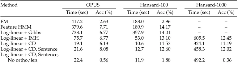
Table 4 reports the accuracy and running time per iteration for exact EM, Feature HMM, and our log-linear models on the OPUS, Hansard-100, and Hansard-1000 data sets. However, on the Hansard-1000 data set, we only applied the contrastive diver-gence and IMH based log-linear models because of its large vocabulary size. Table 2 summarizes the computational complexity of each method; recall thatNF scales with
[image:17.486.53.438.560.669.2]V(theoreticallyNF∈O(V2), although empirically we foundNF∈O(V)). From this, we
Table 4
The running time per iteration and accuracy of decipherment.
Method OPUS Hansard-100 Hansard-1000
Time (sec) Acc (%) Time (sec) Acc (%) Time (sec) Acc (%)
EM 417.2 2.63 188.0 2.96 – –
Feature HMM 379.6 7.71 189.9 14.17 – –
Log-linear + Gibbs 738.1 6.77 357.9 14.01 – –
Log-linear + IMH 75.7 6.77 53.0 13.10 605.5 12.45
Log-linear + CD 19.1 6.13 10.6 11.53 324.1 11.19
Log-linear + CD, Sentence 21.6 8.08 12.7 12.60 458.3 12.02
Log-linear + CD, Sentence,
Table 5
The effect on accuracy of incorporating parallel data for our model (first three columns) and IBM Model 1 and Model 4 (on Hansard-1000 parallel data).
Accuracy (%) Opus Hansard-100 Hansard-1000 IBM Model 1 IBM Model 4
Monolingual-Only 8.08 12.60 12.02 0.00 0.00
10% Parallel 9.45 16.81 13.58 6.74 7.29
20% Parallel 10.81 17.62 13.41 9.67 10.75
[image:18.486.50.435.230.377.2]50% Parallel 15.04 18.83 18.55 20.03 20.40
Table 6
Comparison of MT performance on the OPUS data set.
Method BLEU (%)
EM (Ravi and Knight, 2011) 15.3
EM + Beam (Nuhn and Ney, 2014) 15.7
Feature HMM 18.90
Log-linear + Gibbs 21.43
Log-linear + IMH 21.46
Log-linear + CD 21.36
Log-linear + CD, Sentence 20.71
Log-linear + CD, Sentence, No ortho/len 19.36 Log-linear + CD, Sentence, 10% Parallel 20.83 Log-linear + CD, Sentence, 20% Parallel 21.18 Log-linear + CD, Sentence, 50% Parallel 29.30
can loosely estimate that the Gibbs sampling would take roughly a week to execute 15 iterations, whereas the EM and Feature HMM methods would take roughly a month.
Table 5 reports the accuracy for the methods that utilize parallel data on the three data sets. For comparison, the final two columns of Table 5 report the accuracy of IBM Model 1 and Model 4 (Brown et al. 1993) when trained on the parallel data used in the corresponding Hansard-1000 experiment; to allow for direct comparison, both were evaluated over the same vocabulary as in the Hansard-1000 experiment. Because our training procedure includes random sampling, the results of each run on a given data set can vary. We observe only very small variations between executions, but all reported results for sampling-based methods are the average of 10 separate executions of the system. A bigram language model was used for all the models.
The BLEU scores for translation on the OPUS data set are reported in Table 6. We outperform previous approaches on this data set that use no parallel data. Although we are not aware of any work on the OPUS data set using small amounts of parallel data, Zoph et al. (2016) describe one recent alternative approach to translation with very limited parallel data for Urdu–English. Their hybrid system using a string-to-tree statistical translation model combined with a neural model achieved a BLEU score of 19.1. This result utilized three times as much data as in our experiments; 100% of it was parallel, and the model was pre-trained with a much larger corpus of parallel French– English data.
Table 7
A few examples for which orthographic features helped.
OPUS Hansard-1000
Spanish English French English
excelente excellent criminel criminal
minuto minute particulier particular
silencio silence sociaux social
perfecto perfect secteur sector
9. Discussion and Future Work
We notice that all the feature-based models (both directed Feature-HMM and undi-rected log-linear models) with orthographic and length features outperformed the EM-based decipherment approach. The only log-linear model that performed much worse was the one which lacked the orthographic and length features. This result emphasizes the importance of orthographic features for decipherment between closely related lan-guage pairs. The margin of improvement due to orthographic features was bigger for the Hansard data sets than that for the OPUS data set. This is expected, as French has had a much larger historical influence on English than Spanish has, largely through the Norman Conquest; this is a major cause for the higher lexical similarity between French and English than between Spanish and English. Quantitatively, 42.72% of the pairs in our English–French gold dictionary were within the normalized edit distance threshold used for our corresponding feature, whereas only 20.97% of the English–Spanish pairs were. The contrastive divergence-based log-linear model achieved overall comparable accuracy to the two other sampling approaches (Gibbs and IMH + Gibbs), despite being orders of magnitude faster. Sentence-level sampling was slightly slower, but achieved higher accuracy than bigram-only sampling. Furthermore, the feature-based models resulted in better translations, as they obtained a higher BLEU score on the OPUS data set (Table 6).
Although the orthographic features provide huge improvements in decipherment accuracy, they also introduce new errors. For example, the Spanish word “madre” means “mother” in English, but our model gave the highest score to the English word “made” due to the high orthographic similarity. However, such error cases are rare compared with the improvement.
The accuracies reported here are significantly lower than those achieved by modern supervised methods (and unsupervised methods with large corpora). However, our results required no more than 1,000 lines of data from each language, and preserved accuracy with as little as 100 lines of data. Thus, this method in its current form is most applicable to languages with extremely limited available data. This can include “lost” languages and any of the numerous modern languages that do not have much data easily accessible online. Our model is also very scalable, and can be applied to settings with more data than we experiment with here but still insufficient data for modern embedding-based unsupervised methods.
For understudied languages, our system can also be used to infer the similarity of two languages. The final weight of the edit distance feature can be interpreted as the model’s estimate of similarity. In our experiments, the edit distance weight for the Hansard experiments was roughly four times that of the OPUS experiments, which matches our expectations, given the increased lexical similarity between French and English. For future work, our feature-based models can be extended by allowing local reordering of neighboring words and considering word fertilities (Ravi 2013). We would also like to extend the features to handle languages with different alphabets or sys-tematically different use of certain characters, perhaps using transliteration techniques such as in Knight and Graehl (1998). Finally, we would like to incorporate more flexible non-local features in MRF, which may not be supported by the directed Feature-HMM model.
10. Conclusion
We presented a feature-based decipherment system using latent variable log-linear models. The proposed models take advantage of the orthographic similarities between closely related languages, and outperform the existing EM-based models. The con-trastive divergence–based variant with sentence-level sampling provided the best trade-off between speed and accuracy. We also showed that it can be modified to incorporate parallel data when available, resulting in increased accuracy.
Acknowledgments
We are grateful to the anonymous reviewers for suggesting useful additions. This research was supported by a Google Faculty award and NSF grant 1449828.
References
Ammar, Waleed, Chris Dyer, and Noah A. Smith. 2014. Conditional random field autoencoders for unsupervised structured prediction. InAdvances in Neural
Information Processing Systems (NIPS-27), pages 3311–3319, Montreal.
Artetxe, Mikel, Gorka Labaka, and Eneko Agirre. 2017. Learning bilingual word embeddings with (almost) no bilingual data. InProceedings of the
55th Annual Meeting of the Association for Computational Linguistics
(Volume 1: Long Papers), pages 451–462, Vancouver.
Berg-Kirkpatrick, Taylor, Alexandre Bouchard-C ˆot´e, John DeNero, and Dan Klein. 2010. Painless unsupervised learning with features. InProceedings of the 2010 Meeting of the North American Chapter of the Association for Computational Linguistics (NAACL-10), pages 582–590, Los Angeles, CA.
Brown, Peter F., Stephen A. Della Pietra, Vincent J. Della Pietra, and Robert L. Mercer. 1993. The mathematics of statistical machine translation: Parameter estimation.Computational Linguistics, 19(2):263–311.
parallel corpora. InProceedings of the 29th Annual Conference of the Association for Computational Linguistics (ACL-91), pages 169–176, Berkeley, CA.
Church, Kenneth Ward. 1993. Char align: A program for aligning parallel texts at the character level. In31st Annual Meeting of the Association for Computational Linguistics, pages 1–8, Columbus, OH.
Dempster, A. P., N. M. Laird, and D. B. Rubin. 1977. Maximum likelihood from incomplete data via theEMalgorithm.
Journal of the Royal Statistical Society, 39(1):1–21.
Dou, Qing and Kevin Knight. 2012. Large scale decipherment for out-of-domain machine translation. InJoint Conference on Empirical Methods in Natural Language Processing and Computational Natural Language Learning (EMNLP/CoNLL-12), pages 266–275, Jeju Island.
Dou, Qing, Ashish Vaswani, and Kevin Knight. 2014. Beyond parallel data: Joint word alignment and decipherment improves machine translation. In
Conference on Empirical Methods in Natural Language Processing (EMNLP-14), pages 557–565, Doha.
Dyer, Chris, Jonathan Clark, Alon Lavie, and Noah A. Smith. 2011. Unsupervised word alignment with arbitrary features. In
Proceedings of the 49th Annual Meeting of the Association for Computational Linguistics (ACL-11), pages 409–419, Portland, OR. Haghighi, Aria, Taylor Berg-Kirkpatrick,
and Dan Klein. 2008. Learning bilingual lexicons from monolingual corpora. In
Proceedings of the 46th Annual Meeting of the Association for Computational Linguistics (ACL-08), pages 771–779, Columbus, OH.
Haghighi, Aria and Dan Klein. 2006. Prototype-driven learning for sequence models. InProceedings of the 2006 Meeting of the North American Chapter of the Association for Computational Linguistics (NAACL-06), pages 320–327, New York, NY.
Hinton, Geoffrey. 2002. Training products of experts by minimizing contrastive divergence.Neural Computation, 14(8):1771–1800.
Kneser, Reinhard and Hermann Ney. 1995. Improved backing-off for M-gram language modeling. InInternational Conference on Acoustics, Speech, and Signal Processing (ICASSP), volume 1,
pages 181–184, Detroit, MI.
Knight, Kevin and Jonathan Graehl. 1998. Machine transliteration.Computational Linguistics, 24(4):599–612.
Knight, Kevin and Kenji Yamada. 1999. A computational approach to deciphering unknown scripts. InACL Workshop on Unsupervised Learning in Natural Language Processing, volume 1, pages 37–44, College Park, MD.
Koehn, Philipp and Kevin Knight. 2000. Estimating word translation probabilities from unrelated monolingual corpora using the EM algorithm. InProceedings of the Seventeenth National Conference on Artificial Intelligence (AAAI-00), pages 711–715, Austin, TX.
Nuhn, Malte and Hermann Ney. 2014. EM decipherment for large vocabularies. In
Proceedings of the 52nd Annual Meeting of the Association for Computational Linguistics (ACL-14), pages 759–764, Baltimore, MD.
Nuhn, Malte, Julian Schamper, and Hermann Ney. 2013. Beam search for solving substitution ciphers. InProceedings of the 51st Annual Meeting of the Association for Computational Linguistics (ACL-13), pages 1568–1576, Sofia.
Nuhn, Malte, Julian Schamper, and Hermann Ney. 2015. Unravel–a decipherment toolkit. InProceedings of the 53rd Annual Meeting of the Association for Computational Linguistics (ACL-15), pages 549–553, Beijing.
Quattoni, Ariadna, Michael Collins, and Trevor Darrell. 2004. Conditional random fields for object recognition. InAdvances in Neural Information Processing Systems (NIPS-17), pages 1097–1104, Vancouver. Rapp, Reinhard. 1995. Identifying word
translations in non-parallel texts. In
Proceedings of the 33rd Annual Meeting of the Association for Computational Linguistics (ACL-93), pages 320–322, Cambridge, MA. Ravi, Sujith. 2013. Scalable decipherment for machine translation via hash sampling. In
Proceedings of the 51st Annual Meeting of the Association for Computational Linguistics (ACL-13), pages 362–371, Sofia. Ravi, Sujith and Kevin Knight. 2011.
Deciphering foreign language. In
Proceedings of the 49th Annual Meeting of the Association for Computational Linguistics (ACL-11), pages 12–21, Portland, OR. Snyder, Benjamin, Regina Barzilay, and
Kevin Knight. 2010. A statistical model for lost language decipherment. InProceedings of the 48th Annual Meeting of the Association for Computational Linguistics (ACL-10), pages 1048–1057, Uppsala.
Advances in Natural Language Processing (RANLP), pages 237–248, Borovets. Zhang, Meng, Yang Liu, Huanbo Luan, and
Maosong Sun. 2017. Adversarial training for unsupervised bilingual lexicon induction. InProceedings of the 55th Annual Meeting of the Association for Computational Linguistics (Volume 1: Long Papers), pages 1959–1970, Vancouver.
Zipf, George K. 1949.Human Behaviour and the Principle of Least Effort. Addison-Wesley. Zoph, Barret, Deniz Yuret, Jonathan May,