Munich Personal RePEc Archive
Decomposing the Effects of Monetary
Policy Using an External Instruments
SVAR
Lakdawala, Aeimit
Michigan State University
November 2016
Online at
https://mpra.ub.uni-muenchen.de/80306/
Decomposing the Effects of Monetary Policy Using an External
Instruments SVAR
∗Aeimit Lakdawala†
Michigan State University
This version: November 2016
Abstract
We study the effects of monetary policy on economic activity separately identifying the effects of
a conventional change in the fed funds rate from the policy of forward guidance. We use a structural
VAR identified using external instruments from futures market data. The response of output to a
fed funds rate shock is found to be consistent with typical monetary VAR analyses. However, the
effect of a forward guidance shock that increases long-term interest rates has an expansionary effect
on output. This counterintuitive response is shown to be tied to the asymmetric information between
the Federal Reserve and the public.
Keywords: Monetary policy, Forward Guidance, Identification with External Instruments
JEL: E31, E32, E43, E52, E58
∗I would like to thank James Hamilton, Kurt Lunsford, Michael Bauer, Pascal Paul, Raoul Minetti and seminar
participants at Michigan State, Federal Reserve Bank of Cleveland, IAAE 2016, Midwest Macro 2016 and 2016 Federal Reserve Bank of St. Louis Applied Econometrics conference for useful comments and suggestions. I would also like to thank Mark Gertler and Peter Karadi for generously sharing their data. Matt Schaffer provided excellent research assistance. Online appendix is available athttp://aeimit.weebly.com/uploads/2/5/5/8/25585085/online_appendix_dmp.pdf
1 Introduction
The Federal Reserve has been increasingly using unconventional policy tools in addition to its more
conventional policy tool of setting a target for the federal funds rate. One important new tool is forward
guidance, where the Fed has tried to guide expectations of market participants about the future path
of the fed funds rate. Moreover, the use of forward guidance has been considered especially important
in recent years by policymakers and academics alike.1 While there is theoretical motivation for its use,2
whether or not the Fed’s use of forward guidance policy has been empirically effective remains an open
question. In this paper we aim to study the effects of monetary policy on economic activity with a focus
on disentangling the effect of forward guidance from conventional policy actions.
Following the work of G¨urkaynak, Sack, and Swanson (2005) (henceforth GSS), several studies
have found significant effects of forward guidance on asset prices using high-frequency financial data.
But identifying the effects of forward guidance on measures of economic activity –which are typically
available at a monthly or lower frequency– is more challenging. At this lower frequency, monetary policy
actions are likely to be endogenous with respect to macroeconomic variables and identifying restrictions
are required to estimate the transmission mechanism. A key contribution of this paper is the use of
a structural vector autoregression (SVAR) that not only allows us to estimate the effects of forward
guidance on economic activity but also to compare it with the effects of conventional monetary policy.
We explicitly model two monetary policy tools; a short-term interest rate capturing conventional policy
and a longer term interest rate capturing forward guidance policy. Identification is achieved through
restrictions imposed using the external instruments framework.
We build on the work of Gertler and Karadi(2015) (henceforth GK) that uses federal funds futures
data as an instrument for the structural monetary policy shock in a SVAR. But they have one monetary
policy tool that captures the joint effect of conventional policy and forward guidance. Extending their
framework to two monetary policy tools (with two instruments) requires one additional identifying
restriction. In this paper we lay out two alternative ways of obtaining this extra restriction. The first
1
Federal Reserve officials have put more emphasis on the importance of forward guidance in their communication with the public in the past decade. A good example is the following quote from a 2011 speech by then chairman Ben Bernanke “Forward guidance about the future path of policy rates, already used before the crisis, took on greater importance as policy rates neared zero”. The topic has also received significant attention from the academic literature, see Blinder, Ehrmann, Fratzscher, De Haan, and Jansen(2008) for an excellent survey.
2
strategy relies on placing a zero restriction on the relationship between the structural shocks and the
reduced form residuals. This amounts to a less restrictive version of the recursive ordering commonly
used in the literature. On the other hand, the second strategy involves putting a zero restriction directly
on the relationship between the structural shocks and the instruments. We show how the factor rotation
of futures data proposed by GSS results in instruments that naturally satisfy the requirements of this
second identification strategy.3
For the baseline results in the paper we consider a simple SVAR with output, prices and the two
monetary policy tools: the fed funds rate and the 1 year Treasury rate. A forward guidance shock is
defined as the structural shock to the 1 year rate that is orthogonal to the contemporaneous structural
shock to the fed funds rate. In this framework, any Federal Reserve announcement (on FOMC meeting
days) about future monetary policy decisions that moves long term interest rates (and is orthogonal to
current rate changes) will be captured as forward guidance. It is important to note that this framework
does not explicitly separate out announcements about large scale asset purchases (i.e. quantitative
easing) as is done for example inSwanson (2016).
The response of the economy to a contractionary federal funds rate shock displays an inverted
hump shaped response for output but a more muted price response. The dynamics of output are
consistent with conventional macroeconomic theory (see for example Gal´ı(2008)) and also consistent
with standard results from VAR analyses of monetary policy (see for exampleChristiano, Eichenbaum,
and Evans (1999)).4 However, the response of the economy to a forward guidance shock does not fit
this pattern. Output rises in response to a “contractionary” forward guidance shock, i.e. a shock that
raises the 1 year interest rate. This result also holds when we exclude unscheduled FOMC meetings
from the sample, use narrower or broader windows to construct the instruments, and when we expand
the information set of the VAR to include financial variables.5
We find that this counterintuitive response is driven by the information differences between the
Federal Reserve and the general public, implying a role for Delphic forward guidance as proposed by
Campbell, Evans, Fisher, and Justiniano(2012). They suggest that the Delphic component of the Fed’s
communication about their future intentions also embodies a signal about future economic conditions.
3
Reassuringly, we find that the results are similar for both identification strategies. 4
We found the response of output to be robust in a variety of different specifications but the response of prices often displays the price-puzzle. Thus in this paper we focus primarily on the response of output.
5
To account for this information effect in the SVAR, we construct a measure of Federal Reserve private
information using Greenbook and Bluechip forecast data. We then regress our instruments from futures
market data on this measure and use the residuals as the new instruments. With the instruments
cleansed of the Fed’s private information, we find that output falls in response to a contractionary
forward guidance shock. In a recent survey, Ramey (2016) estimates several VARs and finds that for
certain specifications there exists a similar expansionary effect of “contractionary” monetary policy
shocks. Our results suggest that the effects of forward guidance, specifically related to the release of
Fed private information may be driving this counterintuitive finding in the literature. These results are
consistent with the finding of Miranda-Agrippino (2016) that also emphasizes the role of information
asymmetries.
Our results raise an important issue about the measurement of the effects of forward guidance.
Should the Delphic component of forward guidance be considered a policy tool for the Federal Reserve?
Or alternatively, should the focus just be on studying the effect of Fed communication (about future
interest rate moves) that is unrelated to economic developments?6 In addition to the work ofCampbell,
Evans, Fisher, and Justiniano (2012) and Campbell, Fisher, Justiniano, and Melosi (2016), there is
recent evidence suggesting that the Delphic component is important. Using high-frequency data,
Naka-mura and Steinsson(2015) find what they call a “Fed information effect” where Fed communication has
an effect on agents’ expectations about future economic fundamentals. In a structural DSGE
frame-workMelosi(2015) emphasizes the importance of the “signalling” channel of monetary policy where the
central bank reveals their information about macroeconomic fundamentals. Overall, we view our results
as complementing this literature and highlighting the need for developing structural models where the
Delphic component of forward guidance is explicitly modeled.
This paper is also related to a growing empirical literature that uses SVARs to estimate the effects of
Federal Reserve communication. D’Amico and King(2015) use survey expectations and sign restrictions
in to identify the structural shocks. Bundick and Smith (2016) embed high-frequency futures market
measures of expected policy rates in a SVAR but use a recursive identification scheme. Ben Zeev,
Gunn N, and Khan (2015) use the maximum-forecast error variance framework to identify monetary
shocks following the news shock literature. Finally,Hansen and McMahon(forthcoming) andLucca and
6
Trebbi (2009) study the effects of communication using different versions of computational linguistics
to categorize the content of FOMC communication. There are three key features that differentiate
our framework from this literature. First, we use the external instruments methodology to identify
structural shocks. Second, we explicitly model two monetary policy tools simultaneously to capture
the joint effects of monetary policy. Finally, we use forecast data to control for Federal Reserve private
information.
The paper proceeds by first laying out the econometric framework in section 2. This section also
includes a discussion of the two alternative identification strategies. Next, in section 3 we discuss
how the high-frequency data is used to construct the instruments and how it fits into the external
instruments framework. Sections 4 presents the results from the baseline specification with extended
results presented in section5. In6we investigate the role of Federal Reserve private information and a
concluding discussion is provided in section 7.
2 Econometric Methodology and Identification
Consider the structural VAR where yt is ann x 1 vector of macroeconomic variables andαi and A
arenxn parameter matrices
Ayt=α1yt−1+. . .+αpyt−p+εt (2.1)
The components of the error termsεt are assumed to be uncorrelated with each other and interpreted
as structural shocks. Pre-multiply byA−1 to get the reduced form VAR
yt=δ1yt−1+. . .+δpyt−p+ut (2.2)
where
ut=Bεt (2.3)
and A−1 = B. Also note that E[utu′t] = BB′ = Σ. This reduced form VAR can be estimated in
a straightforward manner. However identification of the impulse responses to the structural shocks
requires an estimate of the matrixB =A−1. This requires further identifying restrictions. In this paper
and Ravn (2013).7
In the external instruments methodology, the key requirements are to find instruments that are i)
correlated with the shocks of interest (monetary policy shocks here), and ii) uncorrelated with the other
structural shocks (shocks to inflation and output). Denote the policy shocks as εpt and the non-policy shocks asεqt. For a given set of instrumentsZt, these two conditions can be formally stated as
E[Ztεp
′
t ] = φ (2.4)
E[Ztεq
′
t ] = 0 (2.5)
The restrictions2.3,2.4 and2.5 can be represented as
B21=
E[Ztup
′
t ]−1E[Ztuq
′
t]
′
B11 (2.6)
where the impact matrixB is given by
B =
B1 B2
, B1 =
B11′ B21′ ′
, B2 =
B12′ B′22 ′
(2.7)
Intuitively, the estimation follows the following three steps. First, the reduced form VAR in equation
2.2is estimated by ordinary least squares regression. Next, the residuals from the non-policy equations
uqt are regressed on the residuals from the policy equations upt, using Zt as instruments. This gives
an estimate of E[Ztup
′
t ]−1E[Ztuq
′
t ]. Finally, the restrictions in equation 2.6 are used to estimate the
relevant columns of the impact matrixB.
If we are interested in identifying the effects of only one shock (i.e. the policy shockεpt in equation2.4 is a scalar), then the econometric framework identifies the impact coefficients up to a sign convention.
However, if there is more than one policy shock of interest, additional restrictions are required. In this
paper, we have two policy tools and two instruments. Next, we discuss how these additional restrictions
can be obtained using two different identification strategies.
2.1 Identification with Two Policy Shocks and Two Instruments The first strategy
im-poses restriction on the relationship between the reduced-form residuals in the policy equation and the
7
structural policy shocks. The second strategy relies on imposing restrictions on how the instruments are
related to the structural policy shocks. In the scalar case, these two strategies are equivalent, however
this is not true in general for more than one policy shock.
2.1.1 Identification Strategy I The first strategy follows the approach taken in Mertens and
Ravn (2013). To clearly see the identification issue we reproduce the key estimating equations from
their approach.
B11S1−1 = I−B12B22−1B21B11−1
−1
(2.8)
B21S1−1 = B21B11−1 I −B12B22−1B21B11−1−1 (2.9)
S1S1′ = I−B12B22−1B21B11−1
I−B12B22−1B21B11−1
′
(2.10)
The estimation of the covariance matrix of the reduced-form VAR together with the instrumental
variables regression provides estimates of B12B22−1, B11B11′ and B21B11−1.8 For the scalar case, this is
enough to identifyS12 from equation2.10and thusS1 up to a sign convention. WithS1 in hand, we can
back outB11 and B21 which give us the column of the impact matrix required for identification. With
more than one policy shock, we cannot obtainS1 from S1S1′.
The first approach involves putting restrictions on thisS1 matrix. Specifically, in this paper we will
impose a triangular structure on S1, so that a simple Cholesky factorization of S1S1′ gives S1. This
triangular assumption imposes zero restrictions on elements of the S1 matrix. To understand what a
restriction onS1 means, consider the following decomposition of the reduced-form residuals.
upt = ηuqt +S1εpt (2.11)
with
B1 =
I+η(I−ζη)−1ζ
(I−ζη)−1ζ
S1 (2.12)
Recall thatεpt and upt are the structural and reduced-form residuals of the two policy equations. Thus a zero restriction on the rowicolumnj element inS1 implies no direct effect of thejth policy shock in
εpt on the ith reduced-form residual in upt. For the application in this paper: εpt′ = hεf ft εf wdt i
where
8
the “f f” superscript refers to the fed funds rate shock and the “f wd” superscript refers to the forward
guidance shock. Then equation2.11 can be written as
uf ft uf wdt
= ηuqt+
S11 S12 S21 S22
εf ft εf wdt
Thus a lower triangular assumption implies that S12 = 0. This means that the structural forward
guidance shock has no direct effect on the reduced form fed funds rate residual after controlling for the
effect of structural shock that is captured throughuqt.
2.1.2 Identification Strategy II The second identification strategy imposes zero restrictions on
the relationship between the structural policy shocks and the instruments. We derive the estimating
equations using an alternative approach (following Lunsford (2015)) to help understand this second
strategy. Recall the relevance and validity conditions of the instrument,E[Ztεp
′
t ] =φand E[Ztεq
′
t] = 0
and that the covariance matrix of the residuals is given byE(utu′t) = BB′. From these equations we
can show that9
E(Ztu′t) = φB1′ (2.13)
E(Ztu′t)
E(utu′t)
−1
E(utZt′) = φφ′ (2.14)
If we have an estimate ofφ, we can back out the relevant columns of the impact matrixB, which is B1
B1 = E(utZt′)(φ′)−1 (2.15)
Again, if there is only one shock thenφ is a scalar and we can estimate it from from equation2.14 up
to a sign convention. But if there arek >1 shocks (and instruments) then φ has k2 unique elements, whileE(Ztu′t) [E(utu′t)]
−1E
(utZt′) is a symmetric matrix with only k(k+1)
2 unique elements. The second
strategy involves putting zero restrictions on φ. We assume that φis triangular and thus a Cholesky
factorization of φφ′ gives φ. The interpretation of a zero restriction on φ is straightforward from the
relevance condition of the instruments. A zero restriction on the rowicolumnjelement inφimplies that
9
thejth structural policy shock in εpt is uncorrelated with theith instrument in Zt. For the application
in this paper we will use two instruments,Zt= [Zt1 Zt2]′. We can now re-write the relevance condition
as
E[Ztεp
′
t ] = φ
E Z
1
tε f f t Zt1ε
f wd t
Zt2εf ft Zt2εf wdt
=
φ11 φ12 φ21 φ22
Thus a triangular identifying assumption that imposes φ21 = 0 implies that E[Zt2εf ft ] = 0. This assumption is justified by finding an instrument Z2 that is uncorrelated with the fed funds rate shock
but correlated with the forward guidance shock. Specifically, we will use high frequency futures market
data and apply the methodology of GSS. This involves performing a rotation of the principal components
to construct a factor that satisfies the above requirement. This factor (labeled the path factor) captures
shocks in longer term rates but is uncorrelated to fed funds rate shocks. The construction of the
instruments is discussed in more detail in section3.2.
3 Data and Instruments
3.1 Macro Data The baseline VAR is a simple 4 variable monthly VAR with a measure of output,
prices and the two monetary policy tools. Economic activity is measured using the Federal Reserve
Board’s index of industrial production. Inflation is measured using the Consumer Price Index. For
the monetary policy variables we use the fed funds rate as representing the current stance of monetary
policy. To capture forward guidance, we use either the 1 year or 2 year Treasury yield. We use 12 lags in
the estimation. In section5, we discuss the robustness of the results to other specifications that include
expanding the VAR by adding unemployment and other financial variables. Additionally, the online
appendix contains more robustness checks where the VAR is estimated with different sample dates.
For the baseline estimates, we use a monthly data set spanning July 1979 to December 2011. The
start date is chosen to correspond to the appointment of Fed chairman Paul Volcker. In monetary VAR
analyses that use only the fed funds rate as the policy tool, it is typical to stop the sample in late 2008
rate we are using the 1 year rate to capture the effects of the unconventional policy tool of forward
guidance. Forward guidance has been used by the Fed throughout the current zero lower bound episode.
However, we stop the sample in late 2011 based on the analysis ofSwanson and Williams(2014). They
show that 1 year and 2 year bond rates were effectively restrained by the zero lower bound constraint
starting in late 2011. In the online appendix we asses the robustness of the results to using alternative
samples.
3.2 Instrument Construction The external instruments methodology requires instruments that
are correlated with the monetary policy shocks but uncorrelated with the non-policy shocks. We follow
the strategy of GK and use high-frequency data from financial markets to construct our instruments.
Based on the work ofKuttner(2001), they use the change in federal funds futures and eurodollar futures
contracts around FOMC meeting dates as the instrument. The idea is that in a small window around
the FOMC announcement there are unlikely to be other events that significantly affect the market’s
expectations of future interest rates.
The crucial difference between this paper and GK is that they use only one policy tool (1 year
rate) to capture the effect of both conventional and unconventional policy. In this paper the goal is to
separate the effects of contemporaneous changes in the fed funds rate from changes in the 1 year rate
due to forward guidance. To construct two instruments that can allow the separate identification of
these two different policy tools, we follow the analysis in GSS to construct two factors from the response
of futures prices.
Let X denote a T x r matrix of the daily change in the futures price on FOMC days, where T is
the number of time periods andr represents the number of futures price changes used. For the baseline
specification, we will use data from both Fed Funds Futures and Eurodollar Futures contracts up to 4
quarters ahead. We can then perform a principal components analysis of the futures price changes
X =FΛ +ηe
where F is a T x kmatrix of principal components, Λ is a k x 1 vector of factor loadings and ηeis an
error term. The idea is to increase the dimension of the principal components (k) until a sufficiently
baseline results we use end of day data. To check the robustness of the baseline results, in section4 we
discuss results using a narrower 30 minute window constructed with intraday data and also a broader
2 day window.
For the principal components estimation we use 5 futures contracts: current-month and
3-month-ahead federal funds futures contracts and the 2-, 3-, and 4-quarter-3-month-ahead Eurodollar futures contracts,
following the analysis in GSS. We use all the FOMC meeting dates starting with January 1991, which
includes both the scheduled and unscheduled meetings. In the online appendix, we provide a full list
of the dates that are used in the construction of the instruments, including labeling the scheduled and
unscheduled meetings. For the baseline specification, we use all the dates except two. We drop two
FOMC meeting observations following Campbell, Evans, Fisher, and Justiniano (2012). The first one
is the unscheduled FOMC meeting on September 17, 2001 following the 9/11 attacks and the second
one is the QE1 announcement at the FOMC meeting on March 18, 2009. In section 4, we re-do the
estimation dropping all the unscheduled FOMC meeting dates and show that the results are similar.10
GSS found that the first two principal components were sufficient to characterize changes in the five
futures contracts mentioned above. Extending the GSS data to 2015, we find the same result. Table1
shows that the first two principal components can explain more than 95% of the variation in the futures
contracts.11 This conclusion is consistent with the work of Campbell, Evans, Fisher, and Justiniano
(2012) who also perform the target and path factor analysis of GSS using daily data.
For identification strategy I, we can directly use the two factors F1 and F2 as the two instruments
in Z in equation 2.4, since the identification restrictions are put on S1. In the reduced form VAR, if
the fed funds rate is ordered before the long term interest rate, then the matrix S1 is lower triangular. Intuitively, this restriction implies that the response to a forward guidance shock is the response to an
exogenous change that changes the long-rate by 1 percentage point but does not directly affect the fed
funds rate (after taking into account the effect from uqt).12 On the other hand, in response to a fed funds rate shock, the long-rate is directly affected in addition to any change that occurs through uqt.
For identification strategy II, we cannot directly use F1 and F2 as instruments. This is because
10
Furthermore, in the online appendix we show that the results are similar when we exclude the 1991-1993 FOMC meetings.
11
The table actually shows the target and path factors which are rotations of the first two principal components. As discussed below, these rotated factors explain the exact same amount of the variation in the futures price changes as the first two principal components.
12
the changes in the futures contracts on FOMC days contain information about both changes in the
current stance of monetary policy (i.e. the fed funds rate) and also the future stance of monetary policy
(i.e. changes in long-term rates due to forward guidance). The two principal components will capture
both these effects. But identification strategy II requires that one of the instruments be uncorrelated
with one of the structural policy shocks. To tackle this issue we rotate the principal components in
a way that one of the factors will be uncorrelated to changes in the current month’s futures contract
price. In other words, this factor will be uncorrelated to surprise changes in the fed funds rate but will
contain information about changes in the longer term interest rate. GSS outline a way to perform this
rotation that naturally fits the required restriction needed for identification strategy II. Label the two
new factors that will be used as instruments in Z as the target factor (Z1) and the path factor (Z2).
The rotation involves finding an orthogonal matrix U such thatZ1 and Z2 explain the same amount of
variation in X as F1 and F2. More importantly, Z2 is uncorrelated to changes in the current month’s futures contract price. We can write the transformation in the following way.
[Z1 Z2] = [F1 F2]U
The details of the rotation computation are provided in the appendix in section 8.2. Going back to
table 1we see that by construction the path factor explains 0% of the variation in the current month’s
futures contract. As the horizon of the futures contract increases the amount of variation explained by
the path factor increases. On the other hand the target factor has more explanatory power at shorter
horizons.
Finally, we need to aggregate up the daily factor data series (either F1 andF2 orZ1 and Z2) to use
them in a monthly VAR. We follow the procedure used in GK, which adjusts for the fact that FOMC
meetings fall on different days in the month. Since we use interest rate data that are measured as
monthly averages, a meeting that falls earlier in the month will have a bigger impact. We first create a
daily series that cumulates the futures price changes for any FOMC meeting that has occurred in the
past month. Next, we compute the monthly average of this daily series. An alternative methodology is
to construct the monthly numbers by weighing the daily FOMC data based on the day of the month
when the FOMC meeting occurred and then summing up any daily data points within a given month.
4 Results
As mentioned above, the baseline specification has four variables: log Industrial production, log
CPI, federal funds rate and the 1 year Treasury rate. The interest rates are used in levels, as is common
in monetary VARs. The baseline sample for the reduced form VAR runs from July 1979 to December
2011, while the structural identification is carried out using futures data from January 1991 to December
2011.
One potential concern with using the external instruments identification strategy is the weak
in-struments problem. To explore the strength of the factors as inin-struments we present the results from
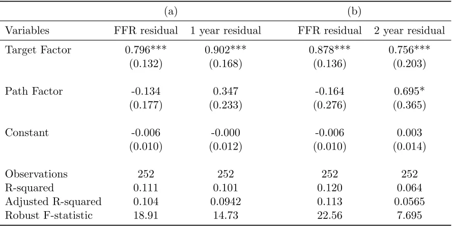
the first stage regressions in table 2, with robust standard errors reported in parentheses. The table
shows the regression of the reduced-from residual from the policy equations on the target and path
factors. For identification strategy I, we don’t need to rotate the principal components to obtain the
target and path factors. The only thing that matters in this case is the joint explanatory power of
the two instruments. But note that the rotation of the principal components preserves the amount
of variation explained by the factors. Thus the F-statistics for the first stage regressions are identical
whether we use the two principal components (F1 andF2) or the rotated factors (Z1 andZ2). However for identification strategy II, we need to use the rotated factors and thus these are reported in the first
stage. The first two columns represent results from using the fed funds rate and 1 year rate as policy
tools, while the second two columns use the fed funds rate and the 2 year rate as policy tools in the
reduced-from VAR. From the first two columns, notice that the robust F-statistics are 18.91 and 14.73.
These numbers are above 10, which is a number recommended byStock, Wright, and Yogo (2002) and
is commonly used as a benchmark in the applied literature.13 The F-statistics are a little lower for the
2 year rate and this motivates the use of the 1 year rate as the policy tool in the baseline results. In
section5, we show that the results are similar using the 2 year rate.
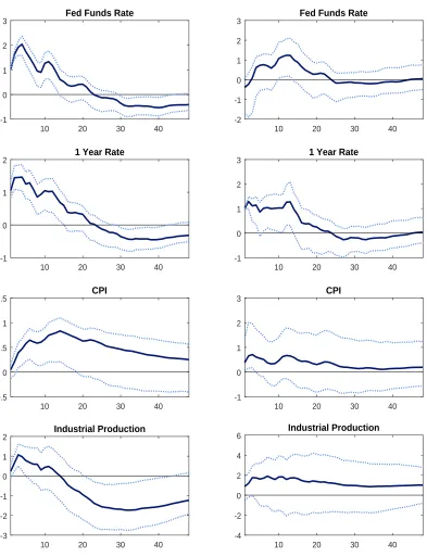
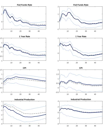
Figure 1shows the impulse responses from the baseline SVAR using the external instruments
iden-tification strategy I, together with 90% confidence intervals. The confidence intervals are computed
using the recursive wild bootstrap following Gon¸calves and Kilian (2004).14 The first column of figure
13
Recent work byLunsford(2015) derives critical values for the F-statistic depending on the level of asymptotic bias in the external instruments framework. However, this paper only considers the case of one policy shock and one instrument which is not directly applicable here. We are not aware of any work that calculates the critical values for more than one policy shock.
14
1 shows the response to a 100 basis point increase to the fed funds rate. This produces a persistent
response with the fed funds rate falling to zero after a year and a half. The 1 year rate rises roughly 50
basis points on impact and falls gradually towards zero around the 2 year mark. Industrial production
falls by .1% on impact and has a U-shaped response with a statistically significant trough close to−2%
being reached around two years. This result is consistent with the prototypical theoretical macro models
and also with VAR analyses of monetary policy, see for example Christiano, Eichenbaum, and Evans
(1999). Even though the CPI falls on impact, it actually rises for about a year, leading to the so-called
price puzzle. While this positive response is not statistically significantly different from zero, it will be
a recurring feature of the various specifications considered in this paper. This result is consistent with
the findings ofBarakchian and Crowe (2013) andRamey(2016) who find price puzzles even after using
futures based identification of monetary policy shocks.15 Thus in this paper we will mostly restrict our
attention to focusing on the response of output.
Next we turn our attention to the second column of figure 1 which shows the effect of a forward
guidance shock that increases the 1 year rate by 100 basis points. After rising on impact, the 1
year rate stays high for about a year before decreasing. The fed funds rate is essentially unchanged on
impact. Note that identification strategy I (or II for that matter) does not restrict the contemporaneous
response of the fed funds rate to be zero in response to a forward guidance shock.16 The rise in the
contemporaneous 1 year rate captures the signal from the Federal Reserve to increase interest rates in
the future and we see this in the response of the fed funds rate which rises slowly for about a year after
the shock. Most notably, CPI and industrial production both rise on impact and continue rising for the
next year. Moreover, this response is statistically significant for both, at least in the first few months.
In figure 2 we show the impulse responses from using identification strategy II. The overall effects are
strikingly similar to identification strategy I with two minor differences. First, the 1 year rate rises more
on impact in response to a fed funds rate shock under strategy II. Second, in response to a forward
guidance shock, output rises on impact and stays a little higher in the medium run relative to strategy I.
Overall, for both identification strategies we conclude that output falls in a hump shaped manner after a
to construct confidence sets for impulse responses in the external instruments framework, but they only consider the case of one policy shock and one instrument.
15
Additionally, in a recent paper using external instruments that focuses on credit spreads,Caldara and Herbst(2016) exclude prices from their baseline VAR specification.
16
fed funds rate shock but rises persistently after a forward guidance shock. Thus a contractionary forward
guidance shock appears to have an expansionary effect on the economy. Some recent studies have also
found expansionary effects of contractionary monetary policy shocks, see for example Barakchian and
Crowe(2013) andRamey(2016). However, in those studies and the overall monetary SVAR literature,
monetary policy is modeled with only one policy tool. Thus one interpretation of the results from figures
1 and 2 is that the counterintuitive finding in the literature can potentially be narrowed down to the
effects coming from forward guidance. However, this result is at odds with standard macro theory and
also the SVAR based forward guidance literature cited above.
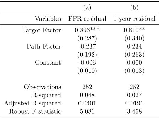
One might be concerned that our result is driven by the inclusion of unscheduled FOMC meeting
dates in the instrument sample. As noted inBarakchian and Crowe(2013) among others, the
unsched-uled FOMC meetings may represent actions by the Federal Reserve that correspond to simultaneous
release of macroeconomic news. To check whether this explains our counterintuitive results, we redo the
analysis leaving out the unscheduled FOMC meetings.17 Table3shows the first stage results from this
specification. Overall, the magnitude and the sign of the coefficients are similar to the baseline case.
The robust F-statistics are lower than the commonly used threshold of 10. While this is potentially
concerning, we find that the impulse responses from this specification are extremely similar to the
base-line specification. These impulse responses are plotted in figure 3 in solid blue lines, with the dashed
black lines showing the baseline case with all the FOMC meetings. After a fed funds rate shock, the
lines in blue show that the response of output is a little lower and that of prices is a little higher relative
to the baseline case. But this difference is small and importantly the responses to a forward guidance
shock are essentially indistinguishable from the baseline case. In the online appendix we address a
related concern about including the FOMC meetings from the early 1990s as part of the futures based
instruments sample. There we show that the results are similar even if we drop the FOMC meetings
from 1991 to 1993.
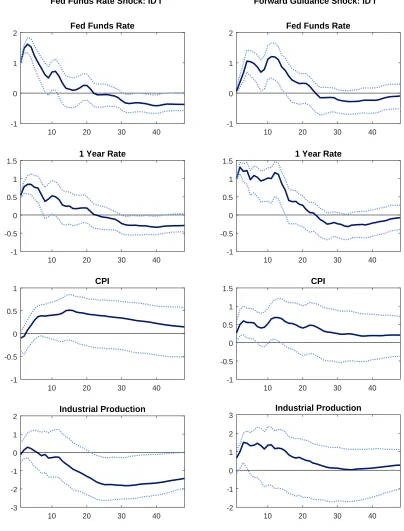
Another potential issue involves the size of the window used to construct the instruments. In the
baseline results we use the end of day data to measure the change in the futures prices on FOMC days.
An alternative is to use a narrower window to measure this change. Notably, GSS and GK both use a
30 minute window around the FOMC announcement. This is motivated by the notion that the narrower
the window the less likely it is that an event other than the FOMC announcement is driving the change
17
in the futures price. On the flip side, some authors have argued that it may take financial markets more
than a couple of hours to digest the FOMC announcement, see for example Hanson and Stein (2015)
who use a two day change. To check the robustness of our results, we estimate our model using both the
30 minute and 2 day window to construct the instruments. Figure4 plots the target and path factors
from these two alternative approaches and compares it with the baseline case. We can see the high
amount of overlap between these measures. As a result, the impulse responses for both specifications
confirm the findings from the baseline case.18 Output falls after a positive shock to the fed funds rate
but rises after a positive shock to the 1 year rate.19 Thus we conclude that the expansionary effect
of a “contractionary” forward guidance shock holds even if we use a narrower or broader window to
construct the instruments or if we exclude unscheduled FOMC meeting dates.
To better understand the source of this effect, we perform various other exercises. The most
impor-tant one turns out to be related to Federal Reserve private information. We find that when we control
for a measure of private information when estimating the VAR, the response of output to a forward
guidance shock no longer displays the puzzling behavior. These results are presented in detail in section
6. But first, we compare the results from this baseline SVAR to specifications that are widely used in
the literature. We would like to understand how our results depend on two main modeling features.
First, how important is the fact that we separate conventional monetary policy from forward guidance?
To evaluate this, we compare our results to a SVAR identified using external instruments but in a
setting where only conventional policy is modeled (using only the fed funds rate) and a setting where
both conventional and unconventional policies are captured by one policy tool. Second, how important
is the external instruments identification methodology in driving the results? To evaluate this, we
com-pare the results from the baseline SVAR with the commonly used recursive (Cholesky) identification
strategy that puts zero restrictions on the matrix governing the contemporaneous relations between the
endogenous variables.
4.1 Comparison of Policy Tools Here we compare our results with monetary SVARs that allow
for only one monetary policy tool. The most common approach in the literature is to just use the fed
funds rate as the policy tool. To do this comparison, we estimate a VAR similar to the baseline case, but
18
For space constraints, the first stage regressions (robust F-statistics remain at or above 10 for both these specifications) and the impulse responses are presented in the online appendix.
19
remove the 1 year rate. We want to use the same identification strategy as the baseline case when making
the comparison. Since the only policy tool is the fed funds rate, the instrument is constructed using just
the current month’s fed funds futures contract (labeled MP1). This is the measure of monetary policy
surprises first constructed in Kuttner (2001) and also used by GSS. As exepected, this measure turns
out to be very similar to the target factor and the correlation between them is 0.98. The first-stage
regression is presented in column (a) of table4. The robust F-statistic from the first stage is sufficiently
high at 78.58.
An alternative approach uses a SVAR to compute the “joint” effect of monetary policy. Here, a
longer term interest rate is the only policy tool and is meant to capture the joint effect of both
conven-tional monetary policy and forward guidance. To do this comparison we use the external instruments
methodology to estimate the baseline SVAR specification but leave out the fed funds rate. This is
essen-tially the specification of GK.20We follow their approach and use the 3 month ahead fed funds futures
contract (labeled FF4) as an instrument for the shocks to the 1 year rate. The first-stage regression is
presented in column (b) of table4. The robust F-statistic from the first stage is 23.11, again implying
no concern of a weak instrument.
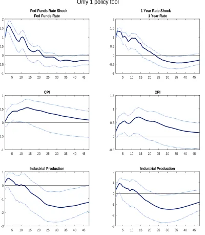
The impulse responses from both these approaches are presented in figure 5. The first column
shows the response to a one percentage point fed funds rate shock, while the second column shows the
responses to a one percentage point shock to the 1 year rate. For both models, output rises slightly
on impact, but then falls and is significantly lower at the two year mark. Importantly, the qualitative
response of output here is very similar to the response of output to a fed funds rate shock in the baseline
specification of this paper, shown in figures 1 and 2. This suggests that studies using only one policy
tool will tend to find effects of monetary policy that mainly capture the effects of conventional monetary
policy. This is not surprising, given that for the majority of our sample period from 1979 to 2011, the
fed funds rate is considered to have been the primary tool of monetary policy.
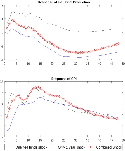
To better understand the result of decomposing monetary policy actions, we plot the response of
output and prices from our baseline model with the corresponding responses from the model where only
the 1 year rate is used as the policy instrument. The dashed black and solid blue lines in figure6 are
responses of output and prices to a funds rate and forward guidance shock respectively from the baseline
20
impulse responses plotted in figure 1. The dotted red line shows the responses to a 1 year rate shock
from figure5. For the CPI, we notice that there are small differences on impact but after a few months
the responses are essentially indistinguishable from one another. On the other hand, there are persistent
differences in the output response. The fed funds rate shock creates a hump-shaped fall in output, while
the forward guidance shock raises output. The combined effect, captured by the red line, creates a fall
in output that lies in between the responses to the individual shocks. Thus an important point is that
studies that do not separately model the effects of the two policy tools may end up misrepresenting the
overall effects of monetary policy.
4.2 Comparison of Identification Strategy Having discussed the results using the external
instruments identification, we want to explore whether using a simpler alternative identification strategy
would give similar results. To this end we compare our results to the recursive Cholesky identification
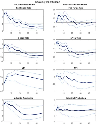
scheme that is frequently used in the literature. In figure 7 we plot the impulse responses using this
recursive Cholesky identification. For this identification scheme, the order of the VAR is potentially
crucial as it determines which elements of the contemporaneous relationship matrix are set to zero.
In the monetary SVAR literature, the convention is to have output and prices ordered before the
monetary policy instrument, see for example Christiano, Eichenbaum, and Evans (1999). In the case
with two policy instruments we have to also order the fed funds rate and the 1 year rate. From the
asset pricing literature there is a clear expectations channel through which movements in the short
rate contemporaneously affect longer rates, while the reverse contemporaneous effect is not entirely
obvious. Thus we use the following ordering: i) Industrial Production, ii) CPI, iii) fed funds rate and
iv) 1 year rate.21 This ordering implies that output and prices do not respond contemporaneously
to either the fed funds rate shock or the 1 year rate shock. Additionally, the fed funds rate does not
respond contemporaneously to the 1 year rate shock but the 1 year rate can respond contemporaneously
to all variables. The impulse responses to a fed funds rate shock and a shock to the 1 year rate are
plotted in figure 7. For the Cholesky identified fed funds rate shock, we notice that the responses
are extremely similar to the baseline responses identified using external instruments, with only small
differences on impact. However for the shock to the 1 year rate, we see that the response of both prices
and output is quite different. The Cholesky identified shock has essentially a zero impact on output after
21
a couple of months. the shapes of the response of output and prices are somewhat similar to the external
instruments case but the differential impact effects result in substantial differences. Overall, this exercise
suggests that the external instruments methodology produces qualitatively and quantitatively different
results from the Cholesky identification. We conclude that the restrictions imposed from the external
instruments methodology imply effects of forward guidance that are quite different from the recursive
identification.
5 Extended Results
In this section we estimate the baseline VAR by adding macroeconomic and financial variables that
are commonly used in the literature. For all the specifications, we find that the main results still hold,
i.e. that effects of a funds rate shock on output are as expected while that of a forward guidance shock
are counter to standard theory. In the next section, we will provide an explanation of this finding
based on information asymmetries, but first we establish the robustness of these findings. For all the
specifications presented in this section, the first stage results are available in the online appendix. In the
same online appendix, we also present the results for different sample periods, i)July 1979 to November
2015, ii)July 1979 to December 2008 and iii)July 1984 to December 2011, all of which are broadly
consistent with the baseline results. Here we focus on results that expand the variables included in the
VAR. We conduct the analysis by adding each variable one at a time to the baseline VAR. This is done
to prevent the number of parameters estimated in the VAR from becoming too large.
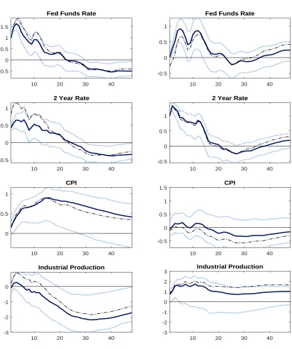
First, we estimate the VAR using the 2 year rate as the monetary policy tool. The first stage
regressions for this specification are provided in table 2. While the F-statistic on the 2 year rate
residual is slightly below 10, the coefficients on both the target and path factor are significant. Figure
8shows the impulse responses using both identification strategy I (solid blue line) and II (dashed black
line). While there are some minor differences among the two identification strategies, the responses
show the same pattern as the baseline results with the 1 year rate.
Next, we add the excess bond premium ofGilchrist and Zakraj˘sek(2012) to the baseline specification,
following GK. One important concern is that the small VAR used for the baseline specification may
be leaving out a lot of information that is actually used by the Federal Reserve in making policy
the VAR. The first stage results (shown in the online appendix) give robust F-statistics above 10 for
both residuals. The solid blue lines in figure9shows the impulse responses from this specification using
identification strategy I. For ease of comparison, the dashed black lines show the responses from the
baseline specification. The excess bond premium rises in response to a contractionary funds rate shock
but has essentially no contemporaneous response to a forward guidance shock. In response to a forward
guidance shock, the rise in output on impact is identical to the baseline case, but it goes back to zero
a little faster when the excess bond premium is included in the VAR. However, the overall responses
of economic activity are very similar. The response of the excess bond premium here is a little muted
relative to GK. Recall that the use of daily data and the use of two monetary policy tools are two
main differences between GK and this paper. We found that the latter of the two is more important in
driving the subdued response.
Next, we add a measure of commodity prices to the baseline specification. In the baseline results
we noted that the response of the CPI displays the well known price puzzle. One common approach in
the literature to account for this price puzzle is to include a measure of commodity prices in the VAR.
The solid blue lines in figure10 shows the impulse responses from this specification using identification
strategy I, with the dashed black line showing the baseline results. Again, the responses of economic
activity are similar with the main difference that the price puzzle is somewhat weakened when we add
commodity prices. The response of commodity prices follows a similar pattern to that of economic
activity, i.e. commodity prices fall in response to a contractionary fed funds rate shock but rise in
response to a forward guidance shock.
In the baseline specification we did not use a direct measure of GDP due to the monthly frequency
of the VAR. Since the unemployment rate is available at this frequency, we add it to the VAR to further
confirm the response of economic activity. The solid blue lines in figure11 show the impulse responses
from this specification using identification strategy I, with the dashed black line showing the baseline
results. As we can see the responses with the unemployment rate added are very similar to the baseline
case. Importantly, the response of the unemployment rate itself is consistent with the story that emerges
from the baseline results, i.e. unemployment rises in response to a contractionary fed funds rate shock
but falls in response to a forward guidance shock. Next we turn to a potential explanation of this
6 Forward Guidance and Federal Reserve Private Information
What explains the counterintuitive response of output to a forward guidance shock? In two recent
papers Campbell, Evans, Fisher, and Justiniano (2012) and Campbell, Fisher, Justiniano, and Melosi
(2016) argue that forward guidance actions can be categorized into Delphic and Odyssean forward
guidance. Odyssean forward guidance fits the conventional definition of forward guidance; a signal from
the Federal Reserve about what it will do to short-term rates in the future. On the other hand, Delphic
forward guidance is a signal that is tied to the release of Federal Reserve information about the future
state of the economy. Importantly, the observed response of the economy to forward guidance shocks
depends crucially on whether these shocks are Odyssean or Delphic in nature. An Odyssean forward
guidance shock that indicates the Fed’s intentions to make short-term rates higher in the future is
unrelated to economic developments and should result in a fall in output and prices. Now consider a
Delphic forward guidance shock that signals the intention of the Fed to raise rates based on revised
forecasts that future economic activity is going to be stronger than expected. In this case, even though
the Fed is going to raise rates, it is a response to an expected pickup in economic activity. Thus it
might be possible to observe output and prices rise after a Delphic forward guidance announcement is
made. Note that in this case the information revealed by the Fed has to be different from the market’s
expectation to have any meaningful effects.
To shed light on this distinction of forward guidance shocks, we redo the VAR analysis using a
“cleansed” measure of the target and path factors that controls for the Delphic part of forward guidance.
The idea is to remove any component from the factors that is capturing the release of private information
by the Federal Reserve about the future state of the economy. To do so we first construct a measure
of Federal Reserve private information following Barakchian and Crowe(2013) and Campbell, Evans,
Fisher, and Justiniano (2012) among others. Next we regress our target and path factors on this
measure of Fed private information. Finally, we use the residuals from the regression as instruments in
the SVAR.
The measure of private information is constructed using two datasets on forecasts. The Greenbook
dataset is used to capture the Fed’s forecasts. This is produced by the Fed’s staff and made available to
FOMC participants a week before the scheduled FOMC meetings. The Greenbook forecasts are made
available to the public. Second, we use the consensus forecasts from the Blue Chip survey as an indicator
of the market’s expectations. The difference between the Greenbook forecasts and the Bluechip forecasts
is used as a measure of Federal Reserve private information. Both the Greenbook and Blue Chip datasets
contain forecasts for macro variables several quarters into the future. We will use forecasts from 1 quarter
ahead up to 4 quarters ahead, since the policy tool for forward guidance in our baseline VAR is the 1
year rate.
Table 5 shows the regressions of the target and path factors on measures of private information
for GDP and CPI and the lagged value of these private information measures. The sample ends in
December 2010, as that is the latest available data for the Greenbook forecasts. Columns (a) and (b)
show the regression coefficients with robust standard errors. The R-squared from both columns is low,
suggesting that Federal Reserve private information only accounts for a small component of the variation
in the futures contracts. Notice that the R-squared is bigger for the path factor regression and that the
adjusted R-squared is actually negative for the target factor regression. Moreover, as can be seen from
column (c), the p-value for the Wald test implies that we fail to reject the null hypothesis that all the
coefficients in the target factor regression are zero. On the other hand, the path factor Wald tests show
that the null hypothesis of all coefficients being zero can be rejected even at the 1% level. Additionally,
testing different groups of parameters for the path factor regression leads to a similar conclusion. Thus
these regressions suggest that the release of private information by the Fed is informative only about the
monetary policy actions at future FOMC meetings as captured in the statement. In the light of these
results we re-estimate the baseline SVAR using as instruments i) the target factor and ii) the residual
from the path factor regression.22
Table6shows the first stage regressions using the cleansed path factor, which involves replacing the
path factor with the residual from the private information regression discussed above. This cleansed
path factor is labeled “Path Factor (Pvt Res)”. The results in the first two columns in table 5 are
remarkably similar to the first stage regressions of the baseline specification shown in table 2. The
Robust F-statistic is above 15 for both the ffr and 1 year residuals. Note that while the coefficient on
the path factor is not significant at the 10% level, it is very close with a p-value of 0.11.
We now use the target factor and the cleansed path factor (“Path Factor (Pvt Res)”) as instruments
22
to identify the two monetary policy shocks.23 The response of the economy to a fed funds rate shock for
both identification schemes is similar to the baseline case and is omitted due to space constraints. The
first column of Figure12 shows the response to a forward guidance shock under the two identification
strategies using this cleansed path factor. The solid blue line shows the responses from identification
strategy I, while the dashed black line shows those under identification strategy II. The dotted blue
lines show the confidence intervals from identification strategy I. The striking result is that now the
contemporaneous response of output to a forward guidance shock is very close to zero and the response
at the 2 and 3 year mark is negative (a little lower in magnitude than −1%). Notice however that
the responses are smaller in magnitude and statistically insignificant for all periods. This is in sharp
contrast to the baseline specification whose results are reproduced in the second column of figure 12
for comparison. In this case, output rises on impact in response to a contractionary forward guidance
shock and the response stays positive for over 3 years.
To summarize, the overall effect of a “contractionary” forward guidance shock is to increase output
while the first column of figure 12 suggests that a contractionary shock controlling for Fed private
information has a small negative impact on output. One interpretation is that the total measured effect
is being dominated by the Delphic component (which is captured by the Fed’s private information).
This reasoning has the underlying assumption that a shock of Delphic type that increases interest rates
is followed by an increase in output. There is a way to check this interpretation in our framework. We
can estimate the SVAR using the fitted component in the private information regression, rather than
the residual component used in figure12. This fitted component is labeled Path Factor (Pvt Fit). The
response of output to this type of forward guidance shock is shown with the dashed red line in figure
13. For comparison, we plot the response from the baseline specification using the dotted black line
and from the Path Factor (Pvt Res) specification using the dashed blue line. These responses match
up well with the interpretation discussed above. A “contractionary” Delphic forward guidance shock
raises output, while an Odyssean one results in a fall in output. The Delphic component dominates
to result in an increase in output in response to a forward guidance shock. Here we must mention an
important caveat regarding the results using the fitted value from the private information regressions.
In table 6, columns (3) and (4) show the first stage regression when using Path Factor (Pvt Fit) as
the instrument. While the F-statistics remain high, the coefficient on the Path Factor (Pvt Fit) is
23
much smaller in magnitude and the standard error is quite large. This results in confidence intervals
for the impulse responses that are much larger for the Path Factor (Pvt Fit) results, especially for the
identification strategy II. Thus we view the results from figure 13 as only suggestive and recommend
interpreting them with a high degree of caution.
Finally, we redo the private information analysis for the case where the unscheduled FOMC meetings
are excluded. The private information regression used to construct the residual and the corresponding
first stage regressions are relegated to the online appendix. The overall results from these two tables are
similar to tables 5 and 6. Again, the response to the fed funds rate shock is similar to the case where
only the scheduled meetings are used and is not included here. Figure14plots the impulse responses to
a forward guidance shock. The first column shows the response under the two identification strategies
using the cleansed path factor (“Path Factor (Pvt Res)”) as instruments to identify the two monetary
policy shocks. The solid blue line shows the responses from identification strategy I, while the dashed
black line shows those under identification strategy II. The dotted blue lines show the confidence intervals
from identification strategy I. The bottom left column shows that output now falls after a contractionary
forward guidance shock, although by less than 1% . Overall, this figure paints the same picture as figure
12. Once the asymmetric information of the Federal Reserve has been stripped out, the effects of forward
guidance no longer generate the counterintuitive response of output.
7 Discussion and Concluding Remarks
What have we learned about the effects of forward guidance in light of the private information
analysis from the previous section? One line of thinking is that we should purge out any effect of Federal
Reserve private information when measuring forward guidance. In other words, only the Odyssean
component of forward guidance should matter when studying the effects of central bank communication.
From this perspective, the results shown in figure 12 suggest that the effects of forward guidance are
small in magnitude and qualitatively in line with conventional theory. However, we would like to raise
two important issues that should be kept in mind when interpreting these results.
First, it is possible that central bank announcements of even the Delphic kind can have direct effects
on the economy. The forecast data used in the previous section highlights the importance of information
agents’ expectations and the economy. Nakamura and Steinsson (2015) find a “Fed information effect”
where Fed communication affects agents’ expectation of future economic activity. Melosi(2015) sets up
a DSGE model with an explicit signalling channel of monetary policy and finds that it has empirically
relevant effects. Finally, Tang (2015) also finds that the empirical patterns in the U.S. inflation data
are consistent with the existence of a signalling channel. While this a nascent literature, it does seem
to suggest that the “signalling/information” channel is important and that the Delphic component of
forward guidance should not be ignored.
Second, it is important to note that the estimates in this paper are based on using data only on
FOMC dates. While it is true that FOMC meeting days are the most important dates on the monetary
policy calendar, there are other occasions on which the Federal Reserve communicates to the public. The
publicly announced events include speeches made by FOMC members, media interviews and testimony
to Congress. Additionally, some information from the Federal Reserve may filter through to the markets
through other sources. A recent paper by Cieslak, Morse, and Vissing-Jorgensen(2015) suggests that
this may even be happening at a bi-weekly frequency. Thus we view our results as measuring only the
partial effect of FOMC communication.
To summarize, in this paper we try to separately identify the effects of conventional monetary policy
from the newer unconventional policy of forward guidance. This is done in a SVAR framework where
the identification of the monetary transmission mechanism is achieved using the external instruments
methodology. Within this framework of multiple policy tools we show that there are two alternative
identification strategies that can be used with two instruments constructed from futures data. While the
effects of fed funds rate shock is consistent with standard macro theory, the effect of forward guidance
shocks on output appears to be a “puzzle”. We show that this puzzle can be explained once the
discrepancies in the forecast of the Federal Reserve and the general public is accounted for. Overall,
our results highlight the need for developing structural models of central bank communication which
incorporate an additional channel through which the release of central bank information can affect
References
Barakchian, S. M., and C. Crowe (2013): “Monetary policy matters: Evidence from new shocks
data,”Journal of Monetary Economics, 60(8), 950–966.
Ben Zeev, N., C. Gunn N, and H. Khan (2015): “Monetary News Shocks,” Carleton Economic
Paper, pp. 15–02.
Blinder, A. S., M. Ehrmann, M. Fratzscher, J. De Haan, andD.-J. Jansen (2008): “Central
Bank Communication and Monetary Policy: A Survey of Theory and Evidence,”Journal of Economic
Literature, 46(4), 910–45.
Bundick, B., and A. L. Smith(2016): “The Dynamic Effects of Forward Guidance Shocks,”Federal
Reserve Bank of Kansas City Working Paper, (16-02).
Caldara, D.,andE. Herbst(2016): “Monetary Policy, Real Activity, and Credit Spreads: Evidence
from Bayesian Proxy SVARs,” .
Campbell, J., J. Fisher, A. Justiniano, and L. Melosi(2016): “Forward Guidance and
Macroe-conomic Outcomes Since the Financial Crisis,” in NBER Macroeconomics Annual 2016, Volume 31.
University of Chicago Press.
Campbell, J. R., C. L. Evans, J. D. Fisher, andA. Justiniano(2012): “Macroeconomic effects
of federal reserve forward guidance ,”Brookings Papers on Economic Activity, pp. 1–80.
Christiano, L. J., M. Eichenbaum,andC. L. Evans(1999): “Monetary policy shocks: What have
we learned and to what end?,” Handbook of macroeconomics, 1, 65–148.
Cieslak, A., A. Morse, andA. Vissing-Jorgensen(2015): “Stock returns over the FOMC cycle,”
Available at SSRN 2687614.
D’Amico, S., and T. B. King (2015): “What Does Anticipated Monetary Policy Do?,” Federal
Reserve Bank of Chicago Working Paper.
Del Negro, M., M. P. Giannoni, and C. Patterson (2015): “The Forward Guidance Puzzle,”
Eggertsson, G. B.,andM. Woodford(2003): “Zero bound on interest rates and optimal monetary
policy,” Brookings Papers on Economic Activity, 2003(1), 139–233.
Gal´ı, J. (2008): “Monetary Policy,” Inflation, and the Business Cycle: An Introduction to the New
Keynesian Framework.
Gertler, M., and P. Karadi (2015): “Monetary Policy Surprises, Credit Costs, and Economic
Activity,” American Economic Journal: Macroeconomics, 7(1), 44–76.
Gilchrist, S., andE. Zakraj˘sek(2012): “Credit Spreads and Business Cycle Fluctuations,”
Amer-ican Economic Review, 102(4), 1692–1720.
Gonc¸alves, S., andL. Kilian(2004): “Bootstrapping autoregressions with conditional
heteroskedas-ticity of unknown form,” Journal of Econometrics, 123(1), 89–120.
G¨urkaynak, R. S., B. Sack,andE. T. Swanson (2005): “Do Actions Speak Louder Than Words?
The Response of Asset Prices to Monetary Policy Actions and Statements,”International Journal of
Central Banking.
Hamilton, J. D.(2003): “What is an oil shock?,” Journal of econometrics, 113(2), 363–398.
Hansen, S., and M. F. McMahon(forthcoming): “Shocking Language: Understanding the
macroe-conomic effects of central bank communication,”Journal of International Economics.
Hanson, S. G., and J. C. Stein (2015): “Monetary policy and long-term real rates,” Journal of
Financial Economics, 115(3), 429–448.
Kuttner, K. N.(2001): “Monetary policy surprises and interest rates: Evidence from the Fed funds
futures market,” Journal of monetary economics, 47(3), 523–544.
Lucca, D. O., and F. Trebbi (2009): “Measuring central bank communication: an automated
approach with application to FOMC statements,” Discussion paper, National Bureau of Economic
Research.
Lunsford, K. G. (2015): “Identifying Structural VARs with a Proxy Variable and a Test for a Weak
Lunsford, K. G.,andC. Jentsch(2016): “Proxy SVARs: Asymptotic Theory, Bootstrap Inference,
and the Effects of Income Tax Changes in the United States,” Discussion paper.
Melosi, L. (2015): “Signaling effects of monetary policy,” .
Mertens, K., and M. O. Ravn (2013): “The dynamic effects of personal and corporate income tax
changes in the United States,” The American Economic Review, 103(4), 1212–1247.
Miranda-Agrippino, S. (2016): “Unsurprising Shocks: Information, Premia, and the Monetary
Transmission,” Unpublished Manuscript, Bank of England.
Montiel-Olea, J. L., J. H. Stock, and M. W. Watson (2016): “Uniform Inference in SVARs
Identified with External Instruments,” .
Nakamura, E.,andJ. Steinsson(2015): “High frequency identification of monetary non-neutrality,”
Discussion paper, National Bureau of Economic Research.
Ramey, V. A.(2016): “Macroeconomic Shocks and their Propagation,”Handbook of Macroeconomics,
forthcoming.
Stock, J. H.,andM. Watson(2012): “Disentangling the Channels of the 200709 Recession,”
Brook-ings Papers on Economic Activity: Spring 2012, p. 81.
Stock, J. H., J. H. Wright, and M. Yogo (2002): “A survey of weak instruments and weak
identification in generalized method of moments,” Journal of Business & Economic Statistics.
Swanson, E. T.(2016): “Measuring the Effects of Unconventional Monetary Policy on Asset Prices,”
Discussion paper, National Bureau of Economic Research.
Swanson, E. T., and J. C. Williams (2014): “Measuring the Effect of the Zero Lower Bound on
Medium- and Longer-Term Interest Rates,”American Economic Review, 104(10), 3154–85.
Tang, J.(2015): “Uncertainty and the signaling channel of monetary policy,” Discussion paper, Federal