Free Energy Problem for the Simulations of the Growth
of Fe
2B Phase Using Phase-Field Method
Raden Dadan Ramdan
1;*, Tomohiro Takaki
2and Yoshihiro Tomita
11
Graduate School of Engineering, Kobe University, Kobe 657-8501, Japan
2Graduate School of Science and Technology, Kyoto Institute of Technology, Kyoto 606-8585, Japan
The present simulation works develop phase-field method to replicate the growth of Fe2B boride from austenite phase. The present works also give a major concern on the free energy driving force problem for this transformation. In order to enhance the reliability of this study, free energy driving force is left as the only variable parameter to be optimized while other parameters were taken from experimental data. Several sets of free energy have been established based on the thermo-chemical database and the assumption that there is a parabolic relationship between free energy of boride/austenite and boron concentration. On the other hand, in order to allow the growth of single Fe2B phase, temperature of 1223 K has been chosen as the evaluated temperature. Based on the comparison of the present numerical results and available experimental data, one set of free energy has been considered to give the appropriate condition that approaching the experimental condition for the growth of Fe2B from austenite phase. [doi:10.2320/matertrans.MRA2008158]
(Received May 9, 2008; Accepted August 18, 2008; Published October 25, 2008)
Keywords: phase-field simulation, boronizing, free energy driving force, line compound
1. Introduction
Boronizing is a kind of thermo-chemical treatment, where boron atom is diffused into the metal substrate to form a hard boride structure on the surface of metal. There are two major types of boride structure, FeB and Fe2B, where the existences
of both phases are depended on the condition of the process such as temperature. The former phase exist when temper-ature of the process is relatively low (below 1223 K), whereas the later phase might exist at higher temperature condition (1223–1373 K) and longer boronizing time.1,2) In addition, FeB phase is also considered to have a higher hardness com-pared to Fe2B phase, however this structure is more brittle
than Fe2B phase.1,3)Therefore, in many cases, it is preferable
to have a single phase of Fe2B rather than having FeB phase
in the boride structure, since the single phase of Fe2B is
considered to offer a higher toughness compared to the structure with the presence of FeB. Overall, boride structure offers a higher hardness compared to other thermo-chemical products, such as boride structure on AISI 5115 steel may produce a hardness of around 1900 HV compared to around 800 HV for the case of carburised layer on the same steel.4) Even-though boronizing process offers a significant im-provement on the quality of material, very limited references can be found on this process. Among them, study on the pack boronizing process1,3,5–7) took the most interest since this process offers a simpler way to produce boride layer. One of the progressive researches on the pack boronizing process have been done by Keddam3,8)who works on the simulation of the growth kinetic of Fe2B, taking into account the
thermodynamic properties of the Fe-B phase diagram and adopting diffusivity of boron by Camposet al.9)In the present study, phase-field method was applied to simulate the growth of single Fe2B boride from the austenite phase and taking
several important experimental data for the pack boronizing of ARMCO iron by Camposet al.,9)which is also used as the
input data for the simulation of boronizing process by Keddam.3)Different with the previous simulations work on boronizing process3,8,9)that use the mass balance equation as the basic model, phase-field model for the growth of boride phase is derived from Ginzburg-Landau free energy func-tional that consider the free energy value from thermo-chemical database and related physical parameters of materials such as interface energy and interface thickness of the corresponding material. This method has been well proved to simulate many kinds of phase transformations, such as austenite-ferrite transformation in steel.10) One important point from this method is the unnecessary of calculating the complex condition of the interface, which might bring difficult problem for the simulation works.
However there is one remaining problem in developing the phase-field simulations for the growth of Fe2B phase, which
is defining its free energy driving force. Since Fe2B is a line
compound that its free energy is defined to be independent of concentration (in the thermodynamic database), therefore there will be no derivative of its free energy on the concentration which is required in constructing the diffusion profile model that couple the phase-field evolution model. One of the common approach to solve this problem is by making an assumption that the free energy of this compound has a parabolic relationship with concentrations.11–13) The present study also adopted the similar approach, and in order to evaluate the reliability of this approach, free energy variable was left as the only variable to be optimized, whereas other important parameters such as interface mobility, diffusion flux and diffusivity coefficient were taken from experimental data and the simulations results was also compared with the related experimental data. The derivation of phase-field model as well as its free energy driving force will be explained in the following subsection.
2. Phase-Field Model
As previously mentioned, phase-field model for the pres-ent work is derived from Ginzburg-Landau free energy
*Graduate Student, Kobe University
Corresponding author, E-mail: [email protected]
functional (eq. (1)),10)where this functional is defined as the functional of free energy density (gð;XB;TÞ) and the gradient energy density (").is the field variable which is set as 1 for boride and 0 for austenite phase, whereasXBand T is the molar fraction of boron and absolute temperature respectively. On the other hand the constant gradient
G¼
Z
V
gð;XB;TÞ þ
"2
2 jrj
2
dV ð1Þ
energy density, ", is related with the interface energy and interface thickness as"¼pffiffiffiffiffiffiffiffiffiffiffiffi3=b.14)Assuming the surface region is < <ð1Þ, we obtainb¼2 tanh1ð12Þ, where is the value of at the onset of surface region ( ¼0:1).
Free energy density in the eq. (1) is constructed by the free energy of boride (GFe2B
m ) and austenite (G
m) as described in the eq. (2). From this equation, pðÞ is an interpolating function which is expressed as, pðÞ ¼3ð10{15þ62Þ,
whereas qðÞ and W are double well potential and the potential height respectively. Potential height is defined as, qðÞ ¼2ð1Þ2, whereas double well potential is related
with the interface energy () and interface thickness () as, W ¼6b=.
gð;XB;TÞ ¼ pðÞGFem2Bþ ð1pðÞÞG
mþWqðÞ: ð2Þ
From the above Ginzburg-Landau free energy functional, the evolution of phase field is derived following the Allen-Cahn equation with the assumption that the total free energy decreases monotonically with time. For the case of one dimensional problem, this derivations produces the following model of phase field evolutions,
@
@t ¼ M
G
¼M
"2r2þ4Wð1Þ
15
2Wð1Þgþ
1 2
: ð3Þ
where g is the chemical driving force which is defined
as gðXB;TÞ ¼GFem2BðXB;TÞ GmðXB;TÞ. This equation
allows the evolution of field variable from¼0(austenite) to¼1(Fe2B), whereMfrom this equation is the kinetic parameter related to the mobility of austenite-boride inter-faceMas
M¼ ffiffiffiffiffiffiffi 2W p
6" M: ð4Þ
Interface mobility is a parameter that relates the interface normal velocity,v, to the driving force. Recent study on the interface mobility by Z.T. Trautt et al.15) consider several types of driving force that causing the movement of interface such as deformation type of driving force, curvature and random walk. Considering the present condition of interface is a flat interface with negligible curvature and there is no contribution of deformation force during the process, there-fore we consider the movement of interface for the present studies is in the type of random walk movement. Correspond to the Z. T. Trauttet al.,15)the interface mobility of random walk type is independent of driving force, therefore the
value of normal velocity of interface is equal with the value of interface mobility for the present study.
The normal velocity of interface is derived from definition of interface position,3) where it is defined that the interface position is a function of kinetic constant, k, and time, resulting an expression of normal velocity of interface as well as interface mobility equal toM ¼k=2pffiffit, wherek is constant which is taken from experimental data by Keddam3)(Table 1) andt is time. For the present work, the interface mobility is kept constant from the initial growth of boride phase, since current understanding of interface mobility consider the interface mobility to have a fixed value and it might increases exponentially with temperature.15–17)
As mentioned in the introduction, defining free energy of boride as a line compound will cause a problem since there is no derivative of its free energy on the concentration. Therefore in order to solve this problem and to find the optimized value of these free energies, both free energy of austenite and boride is approached with the assumption that free energy has a parabolic relationship with concentration and their minimum free energy is similar with the free energy provided by the thermo-chemical database (SGTE database).18) The free energy of austenite is defined as follow
Gm¼GAVþ3:2106ðbXBÞ2; ð5Þ
wherebis the concentration of boron for the minimum free energy of austenite and GAV is the free energy of austenite which is taken from the CALPHAD method for two sub-lattice model as follows
GAV¼yFeyBoGFe:BþyFeyoG
Fe:
þRTyBlnyBþRTylny: ð6Þ
where yFe and yB is the site fraction for iron and boron, respectively. For the present works, in stead of using site fraction, molar fraction values (XFe andXB, molar fraction for iron and boron respectively) are used for the calculation. The site fraction is defined by molar fraction as, yB¼ aXB=cð1XBÞ, whereais equal tocsince we consider the fcc austenite of Fe. On the other handyFe is set as 1 since there is no other alloying element in the matrix. oG
Fe:B is the reference energy term for boron austenite and oG
Fe: is
the reference energy term for vacancy in austenite.oG Fe:B is obtained from the optimization of SGTE database by Van Rompaeyet al.19)as follow
oG Fe:B ¼H
ser B þH
ser
Fe þ4549677:5T: ð7Þ
[image:2.595.304.547.84.155.2]HFeser andHBser is the enthalpy at reference state for iron and boron respectively and are obtained from SGTE database for pure elements.18) On the other hand, the reference
Table 1 Kinetic constant from experimental data by Keddam.3Þ
Temperature (K) k(mms1=2)
1223 0.4584
1253 0.5943
1273 0.6720
energy state for vacancy in austenite, oG
Fe:, in eq. (7) is
obtained from Per Gustafson20) and defined as oG
Fe:¼H
ser
Fe 237:57þ132:4T24:7TlnT
0:0038T25:9E8T3þ77358:5=T: ð8Þ
In order to allow a solubility range in the Fe2B phase, the
chemical free energy of Fe2B is considered to have a
parabolic function of composition,XB, following the similar approach by Huhet al.21)
GFe2B
m ¼FðXB0:33Þ2þoG
Fe2B; ð9Þ
whereF is constant andoGFe2Bis the reference energy term for the stoichimetric composition of Fe2B and is obtained
from the optimization of SGTE database value by Van Rompaeyet al.19)as follow
oGFe2B¼Hser B þ2H
ser
Fe 93363þ481:99T
79:05TlnT0:007T2þ731991T1: ð10Þ
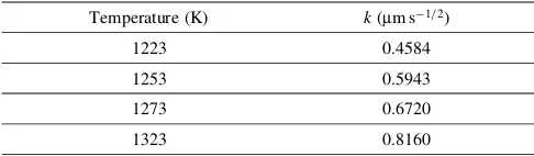
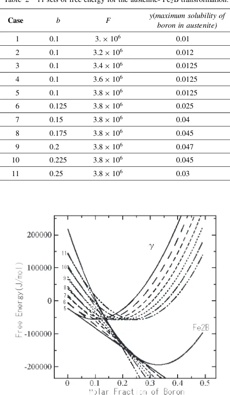
For the present research, 11 sets of free energy will be evaluated to find the optimum condition that is considered to approach the appropriate free energy condition for the transformation of austenite to Fe2B boride phase. The first
[image:3.595.58.286.70.270.2]5 sets of free energy use the fixed value of austenite free energy with b constant (eq. (7)) at 0.1 and F constant (eq. (12)) will be used as the variable parameter to be optimized. These variations results in the sharper curve of boride free energy from the case 1 up to case 5 as can be seen from the common tangent figure of these free energies (Fig. 1). In addition, these variations of free energy also change slightly the boron solubility value as is shown by they term in the Table 2. On the other hand, the last 7 sets of free energy use the optimum value ofFconstant from the first 5 sets of free energy as the fix parameter, and the valued ofb constant as the variable parameter to be optimized. These variations also change the sharpness of the free energy curve and the boron solubility as well, as can be seen in the Fig. 2 and Table 2 respectively. All set of free energies are tabulated in the Table 2.
Regarding the maximum solubility of boron in austenite phase, which is also the results of the construction of common tangent curve of free energy, the present simulations works produce a higher value of this point than that is provided by the available data of this value from the phase diagram. However since phase-field simulations works on the calculation of the growth of one phase from another phase, and for the present works the growth of Fe2B from austenite
phase instead of nucleation of Fe2B phase, alteration of this
point will not effect the calculation. The precise determi-nation of this value is very crucial for the case of nucleation process, where for the case of Fe2B nucleation, this phase
will start to nucleate when the solubility of boron in austenite is exceeded.
3. Boron Diffusion Model
From Ginzburg-Landau free energy functional in the eq. (1), the nonlinear diffusion equation is derived following the Cahn-Hilliard equation as follow
Fe
2B
[image:3.595.307.544.76.482.2]Fig. 1 Common tangent curve for the first 5 sets of free energies with free energy of austenite is kept constant for thebvalue of 0.1 and the free energy of Fe2B is varied with theFvalue as the variable parameter.
Table 2 11 sets of free energy for the austenite- Fe2B transformation.
Case b F y(maximum solubility of
boron in austenite)
1 0.1 3:106 0.01
2 0.1 3:2106 0.012
3 0.1 3:4106 0.0125
4 0.1 3:6106 0.0125
5 0.1 3:8106 0.0125
6 0.125 3:8106 0.025
7 0.15 3:8106 0.04
8 0.175 3:8106 0.045
9 0.2 3:8106 0.047
10 0.225 3:8106 0.045
11 0.25 3:8106 0.03
Fig. 2 Common tangent curve for the sets of free energies with the free energy of Fe2B is kept constant for theFvalue at3:4106and the free energy of austenite is varied with thebvalue as the variable parameter.
[image:3.595.303.549.85.264.2] [image:3.595.320.533.287.482.2]@XB
@t ¼ r MBð;XB;TÞ
@2g
@X2
B
rXBþ
@2g
@XB@
r
; ð11Þ
whereMBis diffusion coefficient of boron, and is defined as a function of diffusion coefficient of boron in austenite, MB, and diffusion coefficient of boron in boride,MFe2B
B , as in the following expression
MBð;XB;TÞ ¼ ðMBFe2BÞ
pðÞðM BÞ
ð1pðÞÞ: ð12Þ
BothMBandMFe2B
B has a temperature dependence function as
MiB¼MoexpðE=RTÞ; ð13Þ
whereMi
Bis the diffusion coefficient of boron in austenite or boride (i¼ or Fe2B), and Mo is the pre-exponential parameter of diffusivity.Movalues for boron in austenite and boride were set at4:4108m2s1and1:13106m2s1
respectively.3)
4. Computational Model
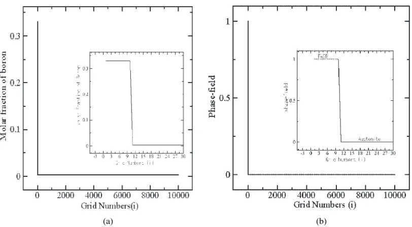
One dimensional finite difference simulations of eqs. (3) and (11) were performed with the solutions of these equations are approached by explicit time difference method. The computational domain is divided into 10000 finite difference grids, where the individual grid size is set at 0.05mm resulting the size of computational domain of 500mm. Initial boron concentration was set at 0.0035 molar fraction of boron in the austenite phase and 0.33 molar fraction of boron in the Fe2B phase (Fig. 3(a)). On the other hand, initial phase-field
variable (Fig. 3(b)) was set as one dimensional equilibrium profile, where it was considered that initially Fe2B phase
(¼1) exist up to grid size of 10 (the origin is ati¼10). Neumann boundary condition is applied at the left side of boron concentration profile, with the gradient value is calculated as the flux (J) of boron entering the surface as J¼D@C=@x, where D is diffusivity of boron in Fe2B,
1:191013m2s1,8) and @C=@x is the average of the gradient of surface concentration on the paste thickness for
the one dimensional case as provided in the experimental data at references8)and we obtained a value of 2 mol/m. On the other hand, zero Neumann boundary condition is applied on the both side of phase-field profile and the right side of concentration profile. The interface thickness,, is set at 8 times of grid size, which is equal to 400 nm, temperature of the process of 1223 K, whereas the interface energy,, is set at 1.0 J/m2.
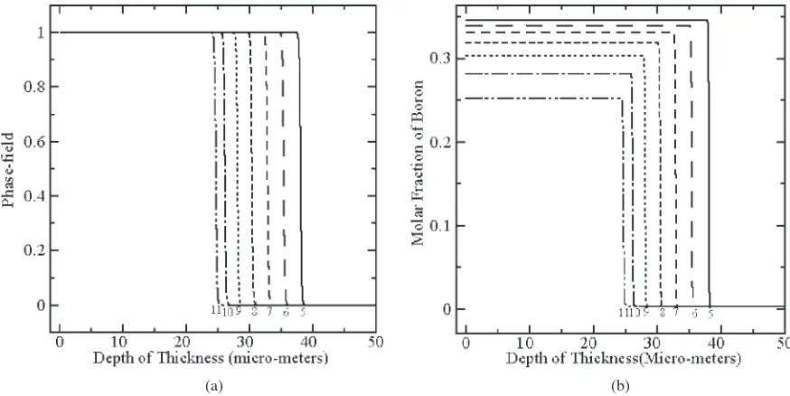
5. Simulation Results and Discussions
Figure 4 illustrates numerical results that replicate the 2 h boronizing process of ARMCO iron for case 1–5 of different set of Fe2B free energy. Experimental data for this
condition3) provide a value of approaching 40mm as the case depth of Fe2B layer which is almost similar with the
depth of thickness obtained by the case 4 and 5 of free energy in the Fig. 4(a). In addition there is a decreasing of depth of thickness from the case 1 up to case 5, which indicates the decreasing of kinetic of the process for these various sets of free energy. This condition is believed due to the lower free energy driving force provides by the higher index (1–5) case of free energy for the composition of boron around 0.3 molar fraction (composition for the case of Fe2B
phase), as also suggested from Fig. 1. It can be seen from this figure that the lower difference of free energy between Fe2B and austenite phase occurs for the composition around
0.3 molar fraction of boron. On the other hand, Fig. 4(b) shows the boron concentration profile for the related boride growth in the Fig. 4(a). It can be seen that case 5 approach the equilibrium condition of Fe2B phase, which is
consid-ered to be around 0.33 molar fraction of boron.1,19) One important point to be noted here is, the equilibrium composition of boron in boride phase as is resulted from the numerical simulations is different with the equilibrium composition as depicted in the common tangent curve (Fig. 1 and 2), where from this curve the equilibrium composition of boron in Fe2B occurs below 0.3 molar
(a) (b)
[image:4.595.96.502.68.292.2]fraction of boron. This situation is considered due to the presence of flux of boron, which is introduced into the system for representing the open system condition of boronizing process, that allow the additional of mass of concentration from the outer of the concerned system. Considering the boronizing system as an open system is very important, since it has also been well-established from the previous research8,22) that boron potential (which is represented by the flux value of boron in the present research) plays an important role in determine the way of boron element impregnates into the inner surface and to the composition of boron as well. Overall, considering the numerical results of Fig. 4(a) and 4(b), the set of free energy for the case 5 is considered to give the appropriate results from these variations of free energy.
By using the optimum F constant of Fe2B free energy
equation from the case 5 as the fixed parameter, evaluation on the variations of austenite free energy has been conducted. Figure 5 shows the numerical results for the case 5–11 of free energy which is also carried out to replicate the 2 h boronizing process of ARMCO iron. It can be seen from Fig. 5(a) that a significant decreasing of depth of thickness occurs from the case 5 to 11, which also indicates a lower free energy driving force occurs in this direction. In addition, case 5 is considered to approach the real kinetic condition since a value of approaching 40mmis obtained for this case, while other cases of free energy show a significant lower value of depth of thickness. On the other hand, Fig. 5(b) shows the numerical results of boron concentration profile for the case 5–11. Case 5,6,7 and 8 produce a considerable value
(a) (b)
Fig. 4 Numerical results that replicate 2 h boronizing process on ARMCO iron, (a) phase-field profile for case 1–5; (b) boron concentration profile for case 1–5.
(a) (b)
Fig. 5 Numerical results that replicate 2 h boronizing process on ARMCO iron, (a) phase-field profile for case 5–11; (b) boron concentration profile for case 5–11.
[image:5.595.87.512.69.286.2] [image:5.595.78.515.339.558.2]that approaching the equilibrium condition for Fe2B phase,
however since only case 5 approaching the experimental kinetic condition of the growth of Fe2B phase (Fig. 5(a)), it
can be concluded that for these variations of free energy, case 5 gives the appropriate free energy that is considered to approach the real free energy driving force for the Fe2B
transformation from austenite phase. Furthermore, since the present variations of free energy that involves the variations of F value (constant that determine the shape of Fe2B free
energy curve) and b constant (constant that determine the concentration for the minimum free energy of austenite) produce a significant influences on the calculations, therefore consideration on these constants is very important for determination of the free energy system of Fe2B
trans-formation. The highlighted common tangent curve of the optimum free energy (case 5), which has also been depicted in the Fig. 1 is shown in the Fig. 6. This construction of free energy as has been previously mentioned produces a maximum solubility of boron in austenite phase at higher value, 0.0125 molar fraction of boron, compared to the 0.00043 molar fraction of boron,19)which is provided in the equilibrium phase diagram. However as has been explained before, since phase-field simulation works on the growth of structure which is not started from the nucleation stage, this deviation will not affect the calculation. In addition, instead of having a line compound of Fe2B, the production of phase
diagram from the present construction of free energy will produce Fe2B phase line which is not independent on the
concentration since the present construction of free energy assumes free energy to be a function of concentration and temperature.
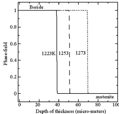
Furthermore, the optimum model obtained in the present simulation works has been used to predict the depth of thickness for different temperature of 1223, 1253 and 1273 K for 2 h of the process. The simulations of these situation is in a good agreement with each condition of experimental works,9) which is around 40mm for 1223 K, between 50– 60mm for temperature of 1253 K and around 70mm for temperature of 1273 K as shown in the Fig. 7.
6. Conclusions
Development of phase-field simulations that replicate the pack boronizing of ARMCO iron has been conducted with the stressing on the evaluation of free energy driving force for the Fe2B transformation from austenite phase. Based on the
available free energy data from SGTE data base and using the assumption that there is a parabolic relationship between free energy of boride and austenite with the boron concentration, 11 set of free energy driving force has been established. By comparing the experimental data of the depth of thickness of Fe2B phase for the similar process and evaluating the boron
concentration profile for each case of free energy, case 5 shows the appropriate numerical results condition which considerably approaching the real condition for the Fe2B
transformation from austenite phase. In addition, the opti-mum model for the present simulations also shows a good agreement for the prediction of depth of thickness of boride for different temperature. However since the present simu-lations process works on the ARMCO iron, which neglecting the presence of alloying element in the steel, therefore it is considered if the present model might works well on the plain carbon steel, where the presence of alloying element is restricted.
REFERENCES
1) L. G. Yu, X. J. Chen, K. A. Khor and G. Sundararajan: Acta Mater.53
(2005) 2361–2368.
2) D. S. Kukharev, S. P. Fisenko and S. I. Shabunya: J. Eng. Phys. Therm.
69(1996) 145–150.
3) M. Keddam: Appl. Surf. Sci.236(2004) 451–45.
4) B. Selc¸uk, R. Ipek and M. B. Karams: J. Mater. Proc. Tech. 141(2003) 189–196.
5) V. Jain and G. Sundararajan: Surf. Coat. Tech.149(2002) 21–26. 6) S. Y. Lee, G. S. Kim and B. S. Kim: Surf. Coat. Tech.177–178(2004)
178–184.
7) C. Li, M. S. Li and Y. C. Zhou: Surf. Coat. Tech.201(2007) 6005– 6011.
8) M. Keddam: Appl. Surf. Sci.253(2006) 757–761.
9) I. Campos, J. Oseguera, U. Figueroa, J. A. Garcia, O. Bautista and Fig. 6 The Highlighted of common tangent curve for the optimum case of
[image:6.595.61.282.67.265.2] [image:6.595.320.526.70.267.2]G. Keleminis: Mater. Sci. Eng. A352(2003) 261–265.
10) A. Yamanaka, T. Takaki and Y. Tomita: Mater. Trans. 47(2006) 2725–2731.
11) S. Y. Hu: Comp. Coupl. Phase Diag. Thermochem.31(2007) 303–312. 12) D. Y. Li and L. Q. Chen: Acta Mater.46(1998) 2573.
13) I. Steinbach: Phys. D94(1996) 135.
14) T. Takaki, T. Hasebe and Y. Tomita: J. Cryst. Growth287(2006) 495–499.
15) Z. T. Trautt, M. Upmanyu and A. Kurma: Science314(2006) 632–635. 16) M. G. Mecozzi, J. Sietsma and S. Van der Zwaag: Comput. Mater. Sci.
34(2005) 290–297.
17) S. I. Vooijs, Y. V. Leeuwen, J. Sietsma and S. V. Zwaag: Metall. Mater. Trans. A31A(2000) 379–385.
18) A. T. Dinsdale: CALPHAD15(1991) 317–425.
19) T. V. Rompaey, K. C. Hari Kumar and P. Wollants: J. Alloy. Compd.
334(2002) 173–181.
20) P. Gustafson: Scandinavian J. Metall.14(1985) 259–267.
21) J. Y. Huh, K. K. Hong, Y. B. Kim and K. T. Kim: J. Elect. Mater.33
(2004) 1161–1170.
22) I. Campos, M. Islas, E. Gonza´lez, P. Ponce and G. Ramı´rez: Surf. Coat. Tech.201(2006) 2717–2723.