On the Third Order Stochastic Dominance for Risk Averse and Risk Seeking Investors with Analysis of their Traditional and Internet Stocks

Munich Personal RePEc Archive

On the Third Order Stochastic

Dominance for Risk-Averse and

Risk-Seeking Investors with Analysis of

their Traditional and Internet Stocks

Chan, Raymond H. and Clark, Ephraim and Wong,

Wing-Keung

The Chinese University of Hong Kong, Middlesex Business School,

Asia University

10 November 2016

On the Third Order Stochastic Dominance for

Risk-Averse and Risk-Seeking Investors with

Analysis of their Traditional and Internet Stocks

Raymond H. Chan

Department of Mathematics, The Chinese University of Hong Kong

Ephraim Clark

Middlesex Business School

Wing-Keung Wong

Department of Finance and Big Data Research Center, Asia University

Department of Economics, Lingnan University

November 10, 2016

Acknowledgements The authors thank Xu Guo for his valuable, manuscript-improving comments. The authors would also like to thank Sheung-Chi Chow and Zhenzhen Zhu in assisting us for the computation and in assisting us in the illustration. The third author would also like to thank Robert B. Miller and Howard E. Thompson for their ongoing counseling and encouragement. Grants from The Chinese University of Hong Kong, Middlesex Business School, Asia University, Lingnan University, and the Research Grants Council (RGC) of Hong Kong have supported this research (project numbers 12502814 and 12500915).

Abstract

This paper presents some interesting new properties of third order stochastic dom-inance (TSD) for risk-averse and risk-seeking investors. We show that the means of the assets being compared should be included in the definition of TSD for both investor types. We also derive the conditions on the variance order of two assets with equal means for both investor types and extend the second order SD (SSD) reversal result of Levy and Levy (2002) to TSD. We apply our results to analyze the investment behaviors on traditional stocks and internet stocks for both risk averters and risk seekers.

Keywords: Third order stochastic dominance, expected-utility maximization, risk aversion, risk seeking, investment behaviors.

1

Introduction

Third-order stochastic dominance (TSD) is becoming an important area of research in

finance. For example, Post, et al. (2015) developed and implemented linear

formula-tions of convex stochastic dominance relaformula-tions based on decreasing absolute risk aversion

(DARA) for discrete and polyhedral choice sets in which DARA is related to the TSD.

In addition, Post and Milos (2016) developed an optimization method for constructing

investment portfolios that dominate a given benchmark portfolio in terms of TSD.

Al-though risk averse investor behavior is the conventional assumption in most financial

research, risk seeking behavior has long been recognized as an important element that

should also be considered. For example, Friedman and Savage (1948) observed investors’

risk-seeking behavior to buy both insurance and lottery tickets. To circumvent this

prob-lem, Markowitz (1952) suggested including convex functions in both the positive and the

negative domains. Williams (1966) found evidence to get a translation of outcomes that

produces a dramatic shift from risk aversion to risk seeking. Tobin (1958) proposed the

mean-variance rules for risk seekers and Kahneman and Tversky (1979) observed

risk-seeking behavior in the negative domain. In this paper we include risk-risk-seeking behavior

in our study of TSD. More specifically, we analyze TSD in the context of both risk-averse

and risk-seeking investors and present some interesting new properties of TSD for both

types of investor. Before we discuss our contribution to the literature, we first discuss the

literature.

for risk averters are concave and increasing while the utility functions for risk seekers are

convex and increasing. In this context stochastic dominance (SD) theory has generated

a rich and growing academic literature. There have been numerous developments in

the theory and application of SD. Most of them relate to second order SD (SSD) and

studies of TSD are relatively rare. Here we list some of the studies on TSD. For example,

Whitmore (1970) first introduced the concept of TSD. Porter,et al. (1973) examined the

factors responsible for the time-consuming nature of SD tests up to the third order and

used their results to develop efficient algorithms for conducting SD tests. Bawa (1975)

proved that the optimal rule for comparing uncertain investments with equal means is

the TSD rule. Fishburn and Vickson (1978) showed that TSD and DARA stochastic

dominance are equivalent concepts when the means of the random alternatives are equal

to one another. Bawa, et al. (1979) developed an algorithm to obtain the second and

third order SD admissible sets by using the empirical distribution function for each stock

as a surrogate for the true but unknown distribution. Eeckhoudt and Kimball (1992)

made the stronger assumption that the distribution of background risk conditional on a

given level of insurable loss deteriorates in the sense of TSD as the amount of insurable

loss increases. In addition, Aboudi and Thon (1994) developed an efficient technique for

determining TSD.

SD theory for risk seekers was developed by Hammond (1974), Meyer (1977), Stoyan

(1983), Levy (2015), and many others. There have also been some studies on TSD that

the convex SD theory for risk averters originally developed by Fishburn (1974) to the

first three orders for both risk averters and risk seekers. Li and Wong (1999) extended

the SD theory and diversification for risk averters developed by Hadar and Russell (1971)

and others by including the TSD and developing the theory to examine the preferences

for risk seekers. Wong (2007) further extended the SD theory of the first three orders to

compare both return and loss.

There are also some applications of TSD theory that link it to other theories. For

example, Gotoh and Konno (2000) showed that many efficient portfolios obtained by the

mean-lower semi-skewness model are also efficient in the sense of TSD. In a study of 24

country stock market indices from 1989-2001, Fong, et al. (2005) showed SSD and TSD

of winner portfolios over loser portfolios. By considering SSD and TSD, Gasbarro, et

al. (2007) showed how switching across funds could increase investor utility. Zagst and

Kraus (2011) derived parameter conditions implying the SSD and TSD of the Constant

Proportion Portfolio Insurance strategy. TSD has also been promoted as a normative

criterion to refine the partial ordering over income distributions (Davies and Hoy, 1994).

In addition, Le Breton and Peluso (2009) introduced the concepts of TSD by using the

Lorenz characterization of the second-degree stochastic order. Ng (2000) constructed

two examples in TSD. Thorlund-Petersen (2001) developed the necessary and sufficient

conditions for TSD.

This paper presents and studies some interesting new properties of SD for risk-averse

(2015) to call the SD for risk seeking investors as risk-seeking SD (RSD). We first discuss

the basic property of SD and RSD linking the SD and RSD of the first three orders

to expected-utility maximization. We then we show that the means of the assets being

compared should be included in the definition of TSD for both risk-averse and risk-seeking

investors, thereby providing a solution to the controversy in the literature on whether or

not the means of the assets being compared should be included in the definition of TSD

for SD and RSD investors.

We extend the second order SD (SSD) reversal result of Levy and Levy (2002) for

two assets that have the same mean to TSD and show that the dominance relationship

can be in the same direction as well as being reversed. Inspired by Levy (2015), 1 _we

explore the relationship between the variances and the integrals of two assets and obtain

the conditions on the order of the variances of two assets for TSD and TRSD under the

condition of equal means. In addition, Rothschield and Stiglitz (1970) proved that if two

assets have the same mean, then there could still be some risk averters that prefer the

asset with the bigger variance. In this paper, we construct an example to show that this

is possible. We then develop the property in which the dominance relationship can be in

the same direction as well as being reversed when the means of the assets are different.

All the properties developed in this paper are illustrated with examples.

Another contribution in this paper is that besides comparing the dominance of the

integrals of two different distributions, we show that the dominance of the means for the

1

Levy (2015) found that for any two assets with equal means, the one having smaller variance is a

distributions should also be checked to draw inference of SD for third order risk averters

and risk seekers. Including “checking the dominance of the means” in the procedure of

testing for third order SD is very important because it can change the results completely.

For example, in our paper, before we include the “means test” in the testing procedure,

our conclusion is “the third-order risk averters prefer investing in the S&P 500 index to

the Nasdaq 100 index in the second sub-period”. However, after we include “the means

test”, our conclusion is“the third-order risk averters are indifferent between the S&P 500

and Nasdaq 100 indices in the second sub-period”.

Finally, we apply the results developed in the paper by comparing the preferences for

traditional and internet stocks for the third-order risk averters and risk seekers. From our

analysis, we conclude that the markets are efficient and there is no arbitrage opportunity

between the S&P 500 and Nasdaq 100 indices in the entire period and in any sub-period,

including any bull run, bear market, the dotcom bubble, and the recent financial crisis.

In general, the third-order risk averters prefer investing in the S&P 500 index to the

Nasdaq 100 index while the third-order risk seekers prefer investing in the Nasdaq 100

index to the S&P 500 index over the entire period as well as many of the sub-periods to

maximize their expected utilities (but not their expected wealth). Interestingly, we find

that both the third-order risk averters and risk seekers are indifferent between the S&P

500 and Nasdaq 100 indices in the bear market during the recent global financial crisis,

However, in the bull run during the dotcom bubble and in the bull run after the recent

and Nasdaq 100 indices while the third-order risk seekers prefer the Nasdaq 100 index to

the S&P 500 index.

In the conclusion we address the question of whether risk seekers actually exist and

discuss how the theory developed in this paper can be used to explain some well-known

financial anomalies such as momentum profits and when efficient mean-variance portfolios

recommended by Markowitz (1952b) are preferred to the equally weighted portfolio

sug-gested by Frankfurter et al. (1971), De Miguelet al. (2009), and others. We also suggest

how it can be used to test other outstanding arguments in the literature.

The rest of the paper is organized as follows. In the next section we present definitions

and notations. Section 3 is devoted to developing the theorems and properties for SD and

RSD. Section 4 provides examples for SD and RSD that illustrate all the properties that

have been developed. In Section 5, we illustrate the theory developed in this paper by

comparing the investment behaviors of both third-order risk averters and risk seekers in

traditional and internet stocks. Section 6 concludes and discusses.

2

Definitions and Notations

We define the “cumulative distribution function” (CDF) of the measureµon the support

Ω = [a, b] ⊂ R as F1(x) ≡ F(x) ≡ µ[a, x] with a < b and µ(Ω) = 1. We also define the

reversed CDF FR

1 (x)≡ µ[x, b] for allx∈ Ω. In addition, we assume that F1 and F1R are

measurable withF1(a) = 0 andF1R(b) = 0. For random variablesX and Y with CDFs F

µF =µX, and the mean of Y, µG=µY, to be

µF =µX =E(X) =

∫ b

a

t d F(t)

and define the following to be used throughout this paper:

Hj(x) =

∫ x

a

Hj−1(y)dy , HjR(x) =

∫ b

x

H_j−R₁(y)dy j = 1,2,3; (2.1)

where H0(x) = H0R(x) =h(x) with H =F orG and h=f or g.

We call Hi the ith-order integrals and we note that the definition of Hi figures in the

development of SD theory for risk averters (see, for example, Quirk and Saposnik 1962).

We callHR

i theith-order reversed integral and we note that the definition ofHiRfigures in the development of SD theory for risk seekers (see, for example, Hammond, 1974). Levy

(2015) called the SD theory for risk seekers risk seeking SD theory and in this paper we

follow Levy to call it risk-seeking SD and denote it by RSD. Risk averters typically have

a preference for assets with a lower probability of loss while risk seekers have a preference

for assets with a higher probability of gain. When choosing between two assets F or G,

risk averters will compare their correspondingith _{order SD integralsF}

i andGi and choose

F if Fi is smaller, since it has a lower probability of loss. In the same vein, risk seekers

will compare their corresponding ith _{order RSD integrals F}R

i and GRi and chooseF if FiR is larger since it has a higher probability of gain. This paper studies the properties of SD

and RSD in detail with an emphasis on third order SD. We now turn to the definitions of

the first-, second-, and third-order SDs as applied to risk averters and RSDs as applied

Definition 2.1 Let F and G be the CDFs of X and Y, X (F) is at least as large as

Y (G) in the sense of:

1. F SD (SSD), denoted by X ≽1 Y or F ≽1 G (X ≽2 Y or F ≽2 G), if and only if

F1(x)≤G1(x) (F2(x)≤G2(x)) for eachx in [a, b], and

2. T SD, denoted by X ≽3 Y or F ≽3 G, if and only if F3(x) ≤ G3(x) for each x in

[a, b] and µX ≥µY,

where F SD, SSD, and T SD stand for first-, second-, and third-order stochastic

domi-nance for risk averters, respectively.

Definition 2.2 Let F and G be the CDFs of X and Y, X (F) is at least as large as

Y (G) in the sense of:

1. FRSD (SRSD), denoted by X ≽R

1 Y or F ≽R1 G (X ≽R2 Y or F ≽R2 G), if F1R(x)≥

GR

1(x) (F2R(x)≥GR2(x)) ∀ x∈[a, b], and

2. TRSD, denoted byX ≽R

3 Y orF ≽R3 G,ifF3R(x)≥GR3(x)∀x∈[a, b]andµX ≥µY,

where FRSD, SRSD, and TRSD stand for first-, second-, and third-order risk-seeking

stochastic dominance, respectively.

We note that one could define strict SD and RSD in Definitions 2.1 and 2.2 by adding

the condition that there is a nonempty subinterval I ⊂[a, b] such that for any x∈ I the

inequalities in Definitions 2.1 and 2.2 are strict. Without loss of generality, we will discuss

Stochastic dominance is considered as especially useful for ranking investment prospects

in conditions of uncertainty because ranking assets is equivalent to maximizing the

ex-pected utility preferences of decision makers with different types of utility functions. The

following definition specifies the relevant types of utility functions:

Definition 2.3 Sets of utility functions,Un and UnR (n= 1,2,3), for risk averters and

risk seekers are:

Un={u: (−1)iu(i) ≤ 0, i= 1,· · · , n} and UnR ={u:u(i) ≥ 0, i= 1,· · · , n},(2.2)

respective, where u(i) _{is the i}th _{derivative of the utility function u.}

We note that in Definition 2.3, U1 = U1R. It is straightforward to extend the theory to

include non-differentiable utilities defined in Definition 2.3 to be non-differentiable (Wong

and Ma, 2008). One may extend the theory to any order n ≥ 1, see, for example, Guo

and Wong (2016). Since we are only interested in the third order in this paper, we stop at

n= 3. Keeping in mind that investors in Un are risk averse while investors inUnR are risk

seeking, it is well known that a negative second derivative for the utility function infers

that investors are risk averse and a positive third derivative for the utility function is a

necessary, but not sufficient condition for decreasing absolute risk aversion (DARA).

In this case, the more wealthy the investor is, the less, on average, he/she is willing

to pay for the insurance against a given risk. That is, ∂r_∂ω(ω) <0. This property is called

decreasing absolute risk aversion (DARA). LetUdbe the set of all DARA utility functions.

It is well-known (Levy, 2015) that ∂r_∂ω(ω) < 0 implies u(3) _{> 0 but U}

Thus, Ud ⊂U3. Menezes, et al. (1980) showed that one CDF is an increase in downside

risk from another if and only if the latter is preferred to the former by all decision makers

with utility functions possessing a positive third derivative. Utility functions in U3 have

non-negative third derivatives, which implies the empirically attractive feature of DARA.

This property is also called prudence (Menezes, et al. , 1980). Post and Levy (2005)

suggested that a third-order polynomial utility function implies that only the first three

central moments of the return distribution (mean, variance, and skewness) are relevant

to investors. On the other hand, Post and Versijp (2007) suggested that TSD efficiency

applies if and only if a portfolio is optimal for some nonsatiable, risk-averse, and

skewness-loving investor. Fong, et al. (2008) commented that TSD adds to risk aversion with the

assumption of a preference for skewness. Crainich, et al. (2013) provided more detailed

information on the shapes of utility functions and their properties for risk averters and

risk seekers.

Levy (2015) pointed out that the prizes of a lottery game are generally positively

skewed because of the small probability of winning a very large prize and the value of

an uninsured house is negatively skewed because of the small probability of a heavy loss

due to a fire or burglary. He argued that people insure their homes because they dislike

negative skewness. On the other hand, people buy a lottery ticket because they like

bigger variance and positive skewness because with a lottery ticket both variance and

skewness increase. He also pointed out that stock returns are generally positively skewed

showed that investors with u(3) _{>0 dislike negative skewness and like positive skewness}

and commented that the behaviors of people buying home insurance, participating in

lotteries, and buying stock conform with the hypothesis that investors dislike negative

skewness and like positive skewness which, in turn, provides support for the hypothesis

that u(3) _{> 0. We also note that the empirical studies by Arditti (1967) and others}

suggested Levy’s argument that investors with u(3) _{> 0 buy stocks. Levy (2015) also}

commented that positive skewness plays a central role in TSD. However, it does not tell

the whole story. He constructed an example in which there is no FSD and no SSD and the

two distributions are symmetrical but yet there is TSD between these two distributions.

According to the von Neumann-Morgenstern (1944) consistency properties, between

two prospectsF andG, investors will preferF toG, or preferXtoY if ∆Eu≡E[

u(X)]

−

E[

u(Y)]

≥0, where E[

u(X)]

≡∫b

a u(x)dF(x) and E

[

u(Y)]

≡∫b

a u(x)dG(x).

3

The Theory

We first state the following basic result linking the SD and RSD of the first three orders

to expected-utility maximization for risk-averse and risk-seeking investors :

Theorem 3.1 Let u be a utility function and F and G be CDFs of X and Y. Then, for j = 1, 2, and 3,

1. X ≽j Y if and only if E[

u(X)]

≥E[

u(Y)]

∀u∈Uj, and

2. X ≽R

j Y if and only if E

[

u(X)]

≥E[

u(Y)]

Several studies have obtained results similar to those in the above proposition for

orders 1 and 2. For instance, Hadar and Russell (1971) and Bawa (1975) established the

FSD and SSD results for continuous utility functions and continuous probability density

functions. For general distribution functions Hanoch and Levy (1969) proved first and

second order SD. Rothschild and Stiglitz (1970, 1971) suggested a condition equivalent to

the SSD results for the special case of cumulative distributions with equal means. Second

order SD for risk averters and risk seekers was discussed by Meyer (1977), Stoyan (1983),

and Levy (2015).

The result in Theorem 3.1 that is still controversial is the result of order 3 because

for order 3 of SD, some (Whitmore, 1970; Bawa, 1975; Levy, 2015) suggest that both

conditions (i) F3(x)≤ G3(x) for each x in [a, b] and (ii) µX ≥µY as stated in Definition

2.1 are necessary while some suggest that condition (ii) is redundant. For example, Schmid

(2005) proved that (i) implies (ii) and thus he suggested that condition (ii) is not necessary.

One could draw similar arguments for RSD. In this paper, we confirm that the condition

µX ≥µY in Definitions 2.1 and 2.2 is necessary in order to obtain the result of order 3 in

Theorem 3.1. Without this condition, the assertions of Theorem 3.1 do not hold for the

case j = 3. We will construct examples in our illustration section to show thatµf ≥µg is

not related to F3(x)≤G3(x). One could easily modify our example to construct another

example to show that µf ≥µg is not related to F3R(x)≥GR3(x).

We are now ready to discuss some other relationships between the third orders of

following theorem:

Theorem 3.2 For any pair of random variables X and Y, for i= 1 and 2, we have:

1. if X ≽i Y, then X ≽i+1 Y ; and

2. if X ≽R

i Y, then X ≽Ri+1 Y.

Theorem 3.2 shows that a hierarchy exists in both SD and RSD relationships and that

the higher orders of SD and RSD can be inferred by the lower orders of SD and RSD but

not vice versa. This suggests that practitioners should report the SD and RSD results to

the lowest order in empirical analyses. We state the well-known hierarchy property in our

paper because it is useful in the proof of other theorems developed in our paper. Levy

and Levy (2002) showed that if F and G are of the same mean, then F dominates G in

SRSD while G dominates F in SSD. We extend their result to include SD and RSD to

the third order SD as stated in the following theorem:

Theorem 3.3 For any pair of random variables X and Y, if F and G have the same mean, which is finite, and if either X ≽2 Y or Y ≽R2 X, then we have

X ≽3 Y and Y ≽R3 X . (3.3)

The proof of Theorem 3.3 is straightforward. Levy and Levy (2002) showed thatX ≽2 Y

if and only ifY ≽R

From Theorem 3.3, we find that the dominance relationships of X and Y are reversed

for SD and RSD. One may wonder whether the relationships of SD and RSD are always

of different directions? The answer is NO. We develop a theorem to show this possibility

as follows:

Theorem 3.4 For any random variablesX andY, if either X ≽1 Y or X ≽R1 Y, then we have

X ≽3 Y and X ≽R3 Y . (3.4)

The proof of Theorem 3.4 could be obtained by applying Lemma 3 in Li and Wong

(1999) and Theorem 3.2 in this paper. One might argue that the third orders SD and

RSD in both Theorems 3.3 and 3.4 are trivial. We get the third orders SD and RSD

because the first or second order SD and RSD relationships exist.

Levy (2015) found that for any two assets X and Y with means µx =µy, he claimed

that σ2

x < σ2y is a necessary condition for TSD. Inspired by Levy’s idea, we explore the relationship between the variances and the integrals of two assets and obtain the following

theorem to state the relationship between the difference of the variances, the difference of

the third-order integrals, and the difference of the third-order reversed integrals for two

different assets under the condition of equal means:

Theorem 3.5 Given µF =µG, we have

G3(b)−F3(b) =GR3(a)−F3R(a) =

1 2

(

σ2_G−σ_F2)

From Theorem 3.5, we can obtain the following corollary to show the necessary and

sufficient conditions on the order of the variances of two assets for both TSD and TRSD

under the condition of equal means:

Corollary 3.1 Given µF =µG, we have

1. F3(b)≤G3(b) if and only if σF2 ≤σG2, and

2. FR

3 (a)≥GR3(a) if and only if σ2F ≥σG2.

From Corollary 3.1, we obtain the following corollary to show the necessary and sufficient

conditions on the order of the variances of two assets for TSD and TRSD under the

condition of equal means:

Corollary 3.2 Given µF =µG, we have

1. if F ≽3 G, then σF2 ≤σ2G, and

2. if F ≽R

3 G, then σ2F ≥σG2.

We note that Levy’s claim that for any two assets X and Y with means µx = µy,

σ2

x < σy2 is a necessary condition for TSD is Part 1 of Corollary 3.2. The converse of Corollary 3.2 is not true. We illustrate that the converse of Corollary 3.2 is not true by

using Example 4.7 as shown in next section.

Corollary 3.2 gives us an impression that for any two distributionsF andG, ifµF =µG,

then if we want to have F ≽3 G, then we must have the condition that σF2 ≤σG2. Is this

and G have the same mean, F may have a lower variance and yet G will be preferred to

F by some risk averse individuals.” We report this result in the following property:

Property 3.1 F and G are two distributions with means µF and µG and variances σ2F

and σ_G2 and there exists a concave utility u∈U2 that E[u(G)]> E[u(F)] if σG2 > σF2.

One could easily show that this does not contradict Corollary 3.2 or any of the

theo-rems/corollaries we developed in our paper. In this paper we will construct Example 4.8

in next section to show that Property 3.1 holds.

One might wonder whether there is any non-trivial third order SD and RSD

relation-ship. Or, more specifically, one might ask: it is possible that there areX andY such that

they do not possess first and second order SD and RSD but there exist third order SD

and RSD and there is a relationship between their third order SD and RSD. Our answer

is YES and we derive one as follows:

Theorem 3.6 If F and G satisfy µF =µG and σ2G=σF2,

then

F ≽3 G if and only if F ≽R3 G .

So far, the theory we developed in this paper from Theorem 3.3 to Theorem 3.6 on the

relationship of SR and RSD is assumed that µF = µG. One may wonder is there any

relationship for SR and RSD in which we do not have to assumeµF =µG? Our answer is

YES and we now develop the following theorems and corollary to show that it is possible

Theorem 3.7 If F and G satisfy σF =σG and µF −µG ≥0, then we have

F ≽3 G=⇒F ≽R3 G .

Theorem 3.8 If F and G satisfy σF =σG and µF −µG ≥0, then we have

F ≽R₃ G=⇒F ≽3 G .

Corollary 3.3 If F and G satisfy σF =σG and µF −µG ≥0, then we have

F ≽R₃ G⇐⇒F ≽3 G .

Theorems 3.7 and 3.8 and Corollary 3.3 show that withµF > µG, it is possible that there

is no FSD or FRSD between F and G, F dominates G in the sense of the third-order

SD and RSD from the same direction. We illustrate in Example 4.9 to show that this is

possible.

4

Illustration

As mentioned above, some papers suggest that the conditionµX ≥µY stated in Definition

2.1 is not necessary to obtain the result in Theorem 3.1. For example, Schmid (2005)

proved that F3(x)≤G3(x) implies µX ≥µY and thus he suggested conditionµX ≥µY is

not necessary. In this paper, we confirm that the condition µX ≥µY in both Definitions

2.1 and 2.2 is necessary in order to obtain the result of order 3 in Theorem 3.1. Without

section, we first construct the following example to illustrate thatµF ≥µG is not related

toF3(x)≤G3(x). One could easily modify our example to construct another example to

show that µF ≥µG is not related toF3R(x)≥GR3(x).

Example 4.1 µF ≥µG is not related to F3(x)≤G3(x)

a. We first construct an example in which G3(x) > F3(x) for all x but yet µG > µF.

Let F(x) =x, the uniform distribution on [0, 1]. Let G(x) be such that

G(x) =

         3x

2 0≤x≤0.24,

0.24 + x

2 0.24≤x≤0.74, 3x

2 −0.5 0.74≤x≤1.

We can see that µG = 0.505>0.5 =µF and G3(x)−F3(x)≥0 for all 0≤x≤1.

b. Next, we construct an example where G3(x) > F3(x) for all x but yet µG < µF.

Again, let F(x) = x, the uniform distribution on [0, 1]. Let G(x) be such that

G(x) =

         3x

2 0≤x≤0.26,

0.26 + x₂ 0.26≤x≤0.76,

3x

2 −0.5 0.76≤x≤1.

We can see that µG = 0.495<0.5 =µF while G3(x)−F3(x)≥0 for all 0≤x≤1.

From this example, we can conclude that (i) G3(x) ≥ F3(x) for all x and (ii) µG < µF

have no relationship at all.

We note that most, if not all, of the examples constructed in this paper could be used

the Production/Operations Management example used by Weeks (1985), Dillinger et al.

(1992), and Wong (2007) as follows:

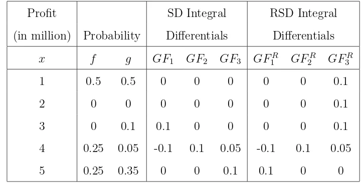
Example 4.2 A production/operations manager make a choice between two invest-ments with profit (x) and their associated probabilitiesf andg as shown in Table 2. From

probabilities f and g, we obtain their SD and RSD integrals Hj and HjR (j = 1,2 and 3)

for H =F and G defined in (2.1) and we define their differentials

GFj =Gj −Fj and GFjR=GRj −FjR . (4.6)

Thereafter, we exhibit the results of the SD and RSD integrals and their differentials for

the first three orders in Table 2.

In this example, our results show that there is no first order SD or RSD between F

and G but we have F ≽j G and G≽R

j F for j = 2 and 3. Thus, this example illustrates Theorem 3.3 (as well as Theorem 3.2).

To illustrate Theorem 3.4, we construct Example 4.3 with Experiment 1 which is used

in Levy and Levy (2002) as follows:

Example 4.3 The gains one month later and their probabilities for an investor who invests $_{10,000 either in stock A or in stock B is shown in the following experiment:}

Experiments 1

Stock A Stock B

Gain (×$1000) Probability Gain (×$1000) Probability Gain (×$1000) Probability

0.5 0.3 -0.5 0.1 1 0.2

2 0.3 0 0.1 2 0.1

We let X and Y be the gain or profit for investing in Stocks A and B with the

corre-sponding probability functions f and g and CDFs F and G, respectively. We depict the

SD and RSD integral differentialsGFj and GFjR for the gain of investing in Stocks A and

B in Table 3 in which GFj and GFjR are defined in (4.6) for j = 1,2 and 3.

From Table 3, we obtain X ≽1 Y and X ≽R1 Y, X ≽2 Y and X ≽R2 Y, as well as

X ≽3 Y and X ≽R3 Y. This example illustrates Theorem 3.4 (as well as Theorem 3.2).

In the above examples, we find that we have both SSD, SRSD, TSD, and TRSD for

a pair of random variables. Is it possible to have TSD and TRSD but no SSD or SRSD?

The answer is YES and this is exactly what Theorem 3.6 tells us. Thus, herewith we

construct an example to illustrate Theorem 3.6 as follows:

Example 4.4 Consider

F(x) = x+ 1

2 , −1≤x≤1 and G(x) =

                            

0 −1≤x≤ −3/4, x+3

4 −3/4≤x≤ −1/4, 1

2 −1/4≤x≤0,

x+1

2 0≤x≤1/4, 3

4 1/4≤x≤3/4,

x 3/4≤x≤1.

Both distributions have the same zero mean. One could easily find for this example

that we do not have F ≽2 G or G≽2 F but we have G≽3 F since the difference G3−F3

is nonpositive. In addition, we can find that F3(b) = G3(b) = 2/3, so the conditions of

Theorem 3.6 hold and we expect G≽R

3 F. Indeed the difference GR3 −F3R is nonnegative which means that G≽R

We now ask: is it possible that we have TSD and TRSD but no SSD or SRSD, and the

conditions of Theorem 3.6 do not hold? The answer is YES and we construct an example

to illustrate this possibility.

Example 4.5 Consider

F(x) =x, 0≤x≤1 and G(x) =

                    

2x 0≤x≤1/6,

1/3 1/6≤x≤5/9,

3x−4/3 5/9≤x≤2/3,

2x−2/3 2/3≤x≤5/6,

1 5/6≤x≤1.

In this example, µF = 0.5 ̸= 0.48148 = µG. Thus, the first condition of Theorem

3.6 does not hold. In addition, one could easily check that we do not have F ≽2 G or

G ≽2 F but we have F ≽3 G since the difference F3 −G3 is nonpositive. Notice that

F3(b)̸=G3(b) and F3R(a)̸=GR3(a), so the second condition of Theorem 3.6 does not hold

either. However, we have F ≽R

3 G since one could check that the difference F3R−GR3 is nonnegative.

In the above examples, we find that we have both TSD and TRSD for a pair of random

variables. Is it possible to have TSD but no TRSD or vice versa? The answer is YES and

we construct two examples in Example 4.6 in which in the first example there exist F

and G such that G≽R

3 F but neither F ≽3 G nor G ≽3 F holds. In the second example

in which there exist F and G such thatF ≽3 G but neither F ≽R3 Gnor G≽R3 F holds.

a. We construct an example in which there existF andGsuch thatG≽R

3 F but neither

F ≽3 G nor G≽3 F holds.

Consider

F(t) =

              

0 0≤t ≤1/10,

2t−1/5 1/10≤t≤1/5,

5t/4−1/20 1/5≤t≤3/5,

3t/4 + 1/4 3/5≤t≤1,

and G(t) = t

In this example, one could easily check that we do not have F ≽3 G or G≽3 F but

we have G≽R

3 F.

b. Next we construct an example in which there exist F and G such that F ≽3 G but

neither F ≽R

3 G nor G≽R3 F holds.

Consider

F(t) =t and G(t) =

              

5t/4 0≤t≤0.4,

3t/4 + 1/5 0.4≤t≤0.8,

0.8 0.8≤t≤0.9,

2t−1 0.9≤t≤1,

One could easily find that F ≽3 G but we do not have F ≽3R G or G≽R3 F.

In Example 4.6 we show that we (i) do not have F ≽3 G or G ≽3 F but have G ≽R3 F

and (ii) do not haveF ≽R

3 Gor G≽R3 F but haveF ≽3 G.

We note that Levy’s claim that for any two assets X and Y with means µx = µy,

σ2

Example 4.7 Consider

f(x) = 1/2 in [−1,1] and g(x) =

                    

0 −1≤ x <−0.9,

1 −0.9≤ x <−0.4,

0 −0.4≤ x <0.4,

1 0.4≤ x <0.9,

0 0.9≤ x ≤1.

We have (i) µF = µG = 0 and (ii) 1/3 = σ2F ≤ σG2 = 0.443, but one could easily check

that F 3 G and F 3 G.

In this paper we construct the following example to show that Property 3.1 holds:

Example 4.8 Consider

G(x) =x, 0≤x≤1 and F(x) =

                                        

5x/4 0≤x≤0.1,

3x/4 + 1/20 0.1≤x≤0.2, x/2 + 1/10 0.2≤x≤0.35,

3x/2−1/4 0.35≤x≤0.5,

3x/2−1/4 0.5≤x≤0.65,

x/2 + 2/5 0.65≤x≤0.8,

3x/4 + 1/5 0.8≤x≤0.9,

5x/4−1/4 0.9≤x≤1.

In this example, µF = µG and σG > σF. Now, we set u(x) = x− 1₈x2 + 1₆x3 − ₁₂1 x4 for

0≥x≥1. Then, one can easily show that u is an increasing concave utility function and

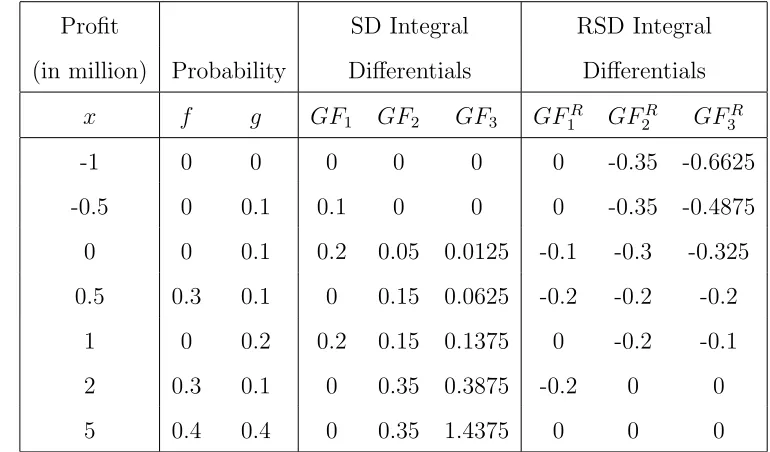
Theorems 3.7 and 3.8 and Corollary 3.3 show that with µF > µG, it is possible that

there is no FSD or FRSD betweenF andG,F dominatesGin the sense of the third-order

SD and RSD from the same direction. We construct the following example to illustrate

this relationship.

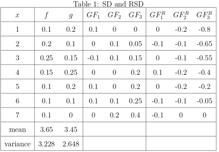
Example 4.9 Let F and G be two assets with probabilities f and g, respectively. One could obtain their SD and RSD integrals Fj, FjR, Gj and GRj by using (2.1). We also

define their differentials as

GFj =Gj−Fj and GFjR =GRj −FjR (4.7)

Thereafter, we exhibit the results of the SD and RSD integral differentials for the first three

orders in the following: The results from Table 1 show that with µF > µG and σF > σG,

there are F ≻j G and F ≻Rj G for j=2 and 3 at the same time.

5

Application

Ofek and Richardson (2003), Scheinkman and Xiong (2003) and Hong, et al.(2006) have

highlighted the insights to be gained from examining investor preferences for traditional

versus internet stocks. There are many studies on this issue with respect to risk averse

investors (See Fong,et al. (2008) and the references therein for more information).

How-ever, as far as we know, there have been no studies that consider both risk averters and

risk seekers, especially for third-order risk averters and risk seekers. To bridge the gap in

Table 1: SD and RSD

x f g GF1 GF2 GF3 GF1R GF2R GF3R

1 0.1 0.2 0.1 0 0 0 -0.2 -0.8

2 0.2 0.1 0 0.1 0.05 -0.1 -0.1 -0.65

3 0.25 0.15 -0.1 0.1 0.15 0 -0.1 -0.55

4 0.15 0.25 0 0 0.2 0.1 -0.2 -0.4

5 0.1 0.2 0.1 0 0.2 0 -0.2 -0.2

6 0.1 0.1 0.1 0.1 0.25 -0.1 -0.1 -0.05

7 0.1 0 0 0.2 0.4 -0.1 0 0

mean 3.65 3.45

variance 3.228 2.648

of risk averters and risk seekers for traditional versus internet stocks, where the S&P 500

index represents the traditional stocks and the NASDAQ 100 index represents the

inter-net stocks. In some existing papers SD tests only compare the dominance of ˆFn(x) with

ˆ

Gn(x) and draw inference for the preference of investors betweenF and G. We note that

this is not good enough. In this paper, we include the test of µX ≥µY, to make the SD

statistics properly test the true SD relationship among the prospects being compared.

5.1

Data

To illustrate the theory we developed in this paper, we use the daily returns of the S&P

500 (S&P) and NASDAQ 100 (Nasdaq). Data for the S&P 500 and NASDAQ 100 were

December 31, 2015. Furthermore, for robustness checking, we divide the entire period into

six sub-periods. In order to compare the results from Fong, et al. (2008), we choose the

same sub-periods used in Fong, et al. (2008), that is, January 1, 1998 to March 9, 2000

(as our second period) and March 10, 2000 to December 31, 2003 (as our third

sub-period). Besides the sub-periods specified by Fong et al. (2008), we identify four other

sub-periods. The first sub-period runs from January 1, 1986 to December 31, 1997. The

fourth sub-period runs from trough to peak of the S&P 500 and the fifth sub-period from

peak to trough. The sixth sub-period is from January 1, 2009 to December 31, 2015. In

this way we can capture and compare the performance between S&P 500 and NASDAQ

100 for different bull and bear markets. One could classify sub-period 1 to be the bull

run before the dotcom bubble, sub-period 2 to be the bull run during the dotcom bubble,

sub-period 3 to be the bear market during the dotcom bubble, sub-period 4 to be the bull

run after the dotcom bubble, sub-period 5 to be the bear market during the recent global

financial crisis, and Sub-period 6 to be the bull run after the recent global financial crisis.

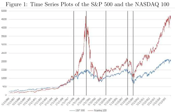
We use Rt, at time t defined asRt= ln(Pt/Pt−1) for the daily returns of S&P 500 and

NASDAQ 100. We display the time series plots of the daily S&P500 and NASDAQ 100

in Figure 1. Figure 1 confirms that, basically, the first, third, and fifth sub-periods are

5.2

Mean Variance Analysis

Before we conduct the SD test, we first apply the MV criterion and display the descriptive

statistics of the data in Table 4 for the entire periods as well as all the sub-periods. Let

X1,· · ·, XnandY1,· · · , Yn be the returns of S&P 500 and Nasdaq 100 indices with means

µ1 and µ2 and variances σ12 and σ22, respectively, for the (sub-)period being studied. The

t statistic is used to test the equality of the means of Xi and Yi while the F statistic is

used to test the ratio of the variances, σ2

1 and σ22 to be unity, respectively.

Markowitz (1952) and Tobin (1958) introduced a MV rule for risk averters such that

for any two returns X and Y with means µX and µY and standard deviations σX and

σY, respectively, X is said to dominate Y by the MV rule for risk averters, (denoted by

X M VRA Y) if µX ≥ µY and σX ≤ σY in which the inequality holds in at least one of

the two. On the other hand, Wong (2007) modified the rule to get the MV rule for risk

seekers such that X is said to dominate Y by the MV rule for risk seekers (denoted by

X M VRS Y) ifµX ≥µY and σX ≥σY in which the inequality holds in at least one of the

two.

From Table 4, the daily mean return of the S&P 500 index is not significantly different

from that of the Nasdaq index neither for the entire period nor for sub-periods 3, 4, 5

and 6. It is only significantly different for sub-period 2. In the other hand, the standard

deviation of daily returns of the S&P index is significantly lower than that of the Nasdaq

index over the entire period as well as over all the sub-periods except subperiod 5 where the

significant. We note that our results of sub-period 2 are consistent with the finding in

Fonget al.(2008) that, on average, the NASDAQ 100 Index outperforms the the S&P 500

index from 1998 to early March 2000. According to the MV criterion, our MV findings

imply that 1) risk averters prefer the S&P 500 to the Nasdaq index for the entire period

as well as all the sub-periods except sub-period 2; (2) risk averters are indifferent between

the S&P 500 and Nasdaq indices in sub-period 2; and (3) risk seekers prefer the Nasdaq

100 index to the S&P 500 index over the entire period as well as over all the sub-periods.

Table 4 further indicates that in general both the S&P 500 and the Nasdaq 100 indices

have significant skewness and kurtosis. Interestingly, the distributions of the returns of

both the S&P 500 and the Nasdaq 100 indices are skewed to the left in the bull markets

and to the right in the bear markets. These results imply that there is a possibility of

greater loss in the bull market even though the mean return is positive and a possibility

of greater gain in the bear market even though the mean return is negative. The presence

of significant skewness (except the skewness of S&P in the fifth sub-period and Nasdaq

100 in the fourth and fifth sub-periods) and kurtosis further supports the hypothesis of

non-normality of the return distributions. The highly significant Jarque-Bera statistic for

the entire period as well as for each sub-period also confirms that the return distributions

of both the S&P 500 and the Nasdaq 100 index are non-normal. This implies that the

conclusions drawn from the MV criterion may be misleading. Thus, we turn to the SD

5.3

SD Analysis

5.3.1 SD Tests for Risk Averters

The tests developed by Davidson and Duclos (DD, 2000), Barrett and Donald (BD, 2003),

and Linton, et al.(LMW, 2005) are the most commonly used statistics to investigate the

preferences of risk averters. Bai, et al.(2015) modified the DD test to include risk seekers

as well as risk averters. Since the test developed by DD is found2 _{to be one of the}

most powerful statistics to test the significance of stochastic dominance, one of the least

conservative in size, and one which is also robust to non-i.i.d. observations, in this paper

we apply only the modified DD tests in our analysis.

For j = 1,2,3; one can test the following hypothesis, H0 : Fj ≡ Gj, against three

alternatives

H1 : F ̸≡j G , H1l F ≻j Gj , and H1r F ≺j G , (5.1)

for the preferences of risk averters. The three hypotheses are equivalent to H1 : Fj(x)̸=

Gj(x) for some x and both H1l : Fj(x)≤Gj(x),∀x and H1r : Fj(x)≥Gj(x),∀x and the

inequality is strict for at least one interval of x.

Suppose that the sample is drawn such that {(fi, gi), i = 1,· · · , m, fk, gl, k = m +

1,· · · , Nf;l = m+ 1,· · · , Ng} where fi and gi are observations drawn from the returns

of the S&P and Nasdaq, denoted by Y and Z with distribution functions F and G,

respectively. The integrals Fj and Gj for F and G are defined in (2.1). For a grid of

pre-selected points {xk, k = 1,· · · , K}, we follow Bai, et al. (2015) to use the following

2

jth _{order modified DD test statistic, T}

j(x) for risk averters to test for H1,H1l, and H1r:

Tj(x) = ˆ

Fj(x)−Gˆj(x)

√

ˆ

Vj(x)

, (5.2)

where

ˆ

Hj(x) =

1

Nh(j−1)! Nh

∑

i=1

(x−hi)j−+ 1,

ˆ

Vj(x) = ˆVFj(x) + ˆVGj(x)−2 ˆVF Gj(x),

ˆ

VF Gj(x) =

1

NfNg((j−1)!)2 m

∑

i=1

(x−fi)j−+1(x−gi)j−+ 1−

m NfNg

ˆ

Fj(x) ˆGj(x),

ˆ

VHj(x) = 1

Nh

[

1

Nh((j−1)!)2 Nh

∑

i=1

(x−hi)+2(j−1)−Hˆj(x)2

]

, H =F, G; h=f, g .

For a pre-designated finite number of values{xk,k = 1,· · · , K}, we test the following

weaker hypotheses: HK

0 : Fj(xk) = Gj(xk) for all xk; H1K : Fj(xk) ̸= Gj(xk) for some

xk; H1Kl : Fj(xk) ≤ Gj(xk) for all xk and Fj(xk) < Gj(xk) for some xk; and H1Kr :

Fj(xk) ≥ Gj(xk) for all xk and Fj(xk) > Gj(xk) for some xk. Under the null hypothesis

HK

0 , the Tj is computed at each grid point and the null hypothesis, H0K, is rejected if

max

k≤K |Tj(xk)|> M K

α/2 for the alternative H1K; min

k≤K Tj(xk)<−M K

α for the alternative H1Kl; and max

k≤K Tj(xk) > M K

α for the alternative H1Kr. We follow Bai, et al. (2011) to get the simulated critical valueMαK by using a bootstrap approach.

In this paper we only examine whether there is any first and third-order SD between

S&P 500 index and Nasdaq 100 index in this paper. We skip reporting the second order

SD because our paper is to study the relationship of the third order SD. The first order SD

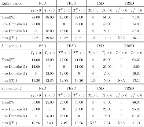
and whether there is any arbitrage opportunity. From Table 5, we observe that there is

no first-order SD (FSD) between the S&P 500 index and the Nasdaq 100 index because

there is 18.00 percent of the first-order modified SD statistic T1 is significantly negative

in negative domain and 22.00 percent of it is significantly positive in positive domain at

the 5 per cent bootstrap simulated critical level. Hence, we conclude that the markets

are efficient and there is no arbitrage opportunity between the S&P 500 and Nasdaq 100

indices in the entire period. In addition, from Table 5, we observe that 8.00 (43.00)

percent of the third-order modified SD statisticT3 is significantly negative in the negative

(positive) domain and none of it is significantly positive at the 5 per cent bootstrap

simulated critical level. Hence, we conclude that there is a dominance of S&P 500 index

and Nasdaq 100 index in terms of third order SD (TSD) at the 5 per cent significance

level, inferring that third-order risk averters prefer investing in the S&P 500 rather than

the Nasdaq 100 index. We also apply the testing procedure by using maxx|Tj(x)|. The

inference drawn from this approach leads to the same conclusion. We now investigate the

preference for risk averters in each of the sub-periods. Table 5 indicates that there are

11.00, 30.00, 32.00, 25.00, 0 and 10.00 percent significantly positive T1 and 12.00, 25.00,

26.00, 26.00, 0 and 1.00 percent of significantly negative T1 in the first, second, third,

fourth, fifth, and sixth sub-periods at the 5 per cent bootstrap simulated critical level.

Thus, there is no FSD between the S&P 500 index and the Nasdaq 100 index at the 5

per cent significance level in any of the sub-periods. This implies that the markets are

indices in any sub-period.

In addition, from Table 5, we find that 25.00, 44.00, 87.00,72.00, 0 and 0 per cent

of T3 are significantly negative in the first, second, third, fourth, fifth and sixth

sub-periods, respectively, but none of it is significantly positive at the 5 per cent bootstrap

simulated critical level for the sub-periods, respectively, implying that the S&P 500 index

stochastically dominates the Nasdaq 100 index in the first, second, third, and fourth

sub-periods but not in the fifth and sixth sub-periods in the sense of TSD.

5.3.2 SD Tests for Risk Seekers

We now turn to examine the preferences of risk seekers between the S&P 500 index and the

Nasdaq 100 index. We follow Bai,et al. (2015) and use the modified DD test statistic for

risk seekers, which we call the risk-seeking DD test statistic. Let {fi} (i = 1,2,· · ·, Nf)

and {gi} (i = 1,2,· · ·, Ng) be observations drawn from the returns of the S&P and

Nasdaq, respectively. For a grid of pre-selected points {xk, k = 1,· · ·, K}and for j = 1,

2 and 3, the jth order risk-seeking DD test statistic, TjR(x), is:

T_jR(x) = ˆ

FR

j (x)−GˆRj(x)

√

ˆ

VR j (x)

where

ˆ

H_jR(x) = 1

Nh(j−1)! Nh

∑

i=1

(hi −x)j−+ 1,

ˆ

V_jR(x) = ˆV_FR_j(x) + ˆV_GR_j(x)−2 ˆV_{F G}R _j(x),

ˆ

V_{F G}R _j(x) = 1

NfNg((j −1)!)2 m

∑

i=1

(fi−x)j−+ 1(gi−x)j−+ 1−

m NfNg

ˆ

F_jR(x) ˆGR_j (x),

ˆ

V_HR_j(x) = 1

Nh

[

1

Nh((j−1)!)2 Nh

∑

i=1

(hi−x)+2(j−1)−HˆjR(x)2

]

, H =F, G; h =f, g;

in which the integrals FjR and GjR are defined in (2.1). For k = 1,· · · , K, the following

hypotheses are tested for risk seekers: HR

0 : FjR(xk) =GRj (xk) for all xk;H1R : FjR(xk)̸=

GR

j(xk) for some xk; H1Rl : FjR(xk) ≥ GRj (xk) for all xk, and FjR(xk) > GRj (xk) for some

xk; and H2Rr : FjR(xk)≤GRj(xk) for all xk and FjR(xk)< GRj (xk) for some xk.

To implement the risk-seeking DD test, TR

j , one can test the following hypotheses at each grid point being computed: HR

0 : FjR ≡GRj, against three alternatives

H₁R F ̸≡R_j G, H₁R_l : F ≻_jRGj, and H1Rr F ≺Rj G . (5.4)

The three hypotheses are equivalent to HR

1 : FjR(x) ̸= GRj (x), for some x and H1Rl :

FR

j (x)≥GRj(x) ,∀xand H1Rr : FjR(x)≤GRj (x),∀xand the inequality is strict for at least one interval of x.

To test the hypotheses (5.4), we reject the null hypothesis HR

0 if max

a<x<b|T R

j (x)|> Mα/R2

for the alternative HR

1 ; max

a<x<b T R

j (x) > MαR for the alternative H1Rl; and min a<x<b T

R j (x) < −M_αR for the alternative HR

1r. We follow Bai, et al. (2011) to get the simulated critical valueMK

Since the conclusion drawn from testing the hypotheses in (5.4) for risk seekers is the

same as that drawn from testing the hypotheses in (5.1) for risk averters for j = 1, we

skip reporting our analysis for testing the hypotheses in (5.4) for j = 1 and only discuss

our analysis for testing the hypotheses in (5.4) for risk seekers forj = 3. We first examine

the preference of third-order risk seekers between S&P 500 and Nasdaq 100 indices in the

entire period. To do so, we employ the third-order RSD statistic, TR

3 , for risk seekers

as stated in (5.3) to analyze the preferences of the third-order risk seekers between S&P

500 index and Nasdaq 100 index and report the result in Table 5. From the table, we

find that 14.00 (57.00) percent of TR

3 is significantly negative at the positive (negative)

domain, and no portion of TR

3 is significantly positive at the 5 percent significant level,

implying that Nasdaq 100 index TRSD dominates S&P 500 index in the entire period.

We now examine the preferences of third-order risk seekers between the S&P 500

and the Nasdaq 100 indices in all the sub-periods. From Table 5, we find that 64.00,

86.00, 56.00, 75.00, 0 and 59.00 percent of TR

3 are significantly negative and none of it

is significantly positive at the 5 per cent bootstrap simulated critical level for the first,

second, third, fourth, fifth, and sixth sub-periods, respectively. This implies that the

Nasdaq 100 index TRSD dominates the S&P 500 index at the 5 per cent significant level

in all the sub-periods except the fifth subperiod.

Overall, the results from the SD tests for both risk averters and risk seekers imply that

the markets are efficient, and there is no arbitrage opportunity between the S&P 500 and

bull run, bear market, the dotcom bubble, and the recent financial crisis. Nevertheless,

the third-order risk averters prefer investing in the S&P 500 index to the Nasdaq 100

index while the third-order risk seekers prefer investing in the Nasdaq 100 index to the

S&P 500 index in the entire period as well as in the first, second, third, and fourth

sub-periods. However, both the third-order risk averters and risk seekers are indifferent

between the S&P 500 and Nasdaq 100 indices in the fifth sub-period. Last, the third-order

risk averters are indifferent between the S&P 500 and Nasdaq 100 indices but the

third-order risk seekers prefer investing in the Nasdaq 100 index to the S&P 500 index in the

sixth sub-period.

5.3.3 Completed SD Tests for Risk Averters and Risk Seekers

The conclusion highlighted in italic in Section 5.3.2 is drawn by conducting the jth _order

modified DD test statistic, Tj(x), in (5.2) and the risk-seeking DD test statistic, TjR(x),

in (5.3). We note that this is the approach recommended by Bai,et al. (2015) and others

and has been used in several studies. For example, Qiao,et al. (2012) apply this approach

and conclude that spot dominates futures for risk averters while futures dominates spot

for risk seekers in the sense of the second and third order SD. We now analyze whether

this approach is correct.

We note that this is correct for j = 1 and 2 but not correct for j = 3. To see why

this is not correct for j = 3, one can refer to Part 2 of Definition 2.1 that X ≻3 Y or

F ≻3 G if and only if (i) H01 : F3(x) ≤ G3(x) for each x in [a, b], F3(x) < G3(x) for at

least one interval of x in [a, b], and (ii) H2

tells us that X ≻R

3 Y or F ≻R3 G if and only if (i*) H01∗ : F3R(x) ≥ GR3(x) ∀ x ∈ [a, b],

FR

3 (x)> GR3(x) for at least one interval of x in [a, b], and (ii) H02 :µX ≥µY. The conclusion highlighted in italic in Section 5.3.2 is obtained by testing H1

0 for risk

averters and H1∗

0 for risk seekers but the hypothesis that H02 µX ≥ µY has not been tested. Thus, in order to complete the SD tests, we must test the hypothesisH2

0 whether

µX ≥µY. To do so, we need to consider the joint Type I error rate to test for bothH01 and

H2

0 or to test for bothH01∗ andH02, that is, the probability that a randomly chosen sample

(of the given size, satisfying the appropriate model assumptions) will give a Type I error

for at least one of the hypothesis tests performed. One easy approach to fix the problem is

to use the Bonferroni correction method (Bonferroni, 1935).3 _{The Bonferroni correction}

method is based on the idea that if an experimenter is testing m hypotheses, then one

way of maintaining the family-wise error rate is to test each individual hypothesis at a

statistical significance level of 1/m times what it would be if only one hypothesis were

tested. So, if the desired significance level for the whole family of tests should be (at most)

α, then the Bonferroni correction would test each individual hypothesis at a significance

level of α/m. In our case, a trial is testing two hypotheses with a desired α = 0.1, then

the Bonferroni correction would test each individual hypothesis at α= 0.1/2 = 0.05.

The conclusion drawn in Section 5.3.1 for risk averters is obtained by testing H01 for

risk averters. In order to complete the SD test for risk averters, we have to test for the

hypothesis that H2

0 µX ≥ µY. The result for testing H02 µX ≥ µY has already been

3

Besides using the Bonferroni correction method, there are some other multiple comparison approaches

reported in Table 4. From the table, we find that the daily mean return of S&P 500 index

is not significant different from that of the Nasdaq 100 index for the entire period as well

as for any sub-period except Sub-period 2 from Jan 1, 1998 to Mar 9, 2000 – a period of

the bull market for the dotcom bubble in which the daily mean return of S&P 500 index

is significantly smaller than that of the Nasdaq 100 index at α= 0.05.

Thus, atα= 0.10, all the conclusion drawn in Section 5.3.1 for risk averters is correct

except that in Subperiod 2 in which we have to change the original conclusion:

“the third-order risk averters prefer investing in the S&P 500 index to the Nasdaq 100

index in the second sub-period”

to

“the third-order risk averters are indifferent between the S&P 500 and Nasdaq 100

indices in the second sub-period”.

On the other hand, the conclusion drawn in Section 5.3.2 for risk seekers is obtained

by testingH1∗

0 for risk seekers but the hypothesis H02 µX ≥µY has not been tested. Thus, in order to complete the SD test for risk seekers, we have to test for the hypothesis that

H2

0 µX ≥ µY. The result for testing H02 µX ≥ µY has already been reported in Table 4. From the table, we conclude that the daily mean return of the Nasdaq 100 index is either

the same or bigger than that of the S&P 500 index. Thus, atα= 0.10, all the conclusion

drawn in Section 5.3.2 for risk seekers holds.

Based on this, we correct the conclusion for both risk averters and risk seekers as

Overall, the result from the SD tests for both risk averters and risk seekers implies that

the markets are efficient, and there is no arbitrage opportunity between the S&P 500 and

Nasdaq 100 indices in the entire period and in any sub-period, including any bull run, bear

market, the dot-com bubble, and the recent financial crisis. Nevertheless, the third-order

risk averters prefer investing in the S&P 500 index to the Nasdaq 100 index while the third

order risk seekers prefer investing in the Nasdaq 100 index to the S&P 500 index in the

entire period as well as in the first, third, and fourth sub-periods. However, both the third

order risk averters and risk seekers are indifferent between the S&P 500 and Nasdaq 100

indices in the fifth sub-period. Finally, the third-order risk averters are indifferent between

the S&P 500 and the Nasdaq 100 indices but the third-order risk seekers prefer investing

in the Nasdaq 100 index to the S&P 500 index in the second and sixth sub-periods.

6

Concluding Remarks

This paper develops and studies several interesting new properties of TSD for risk-averse

and risk-seeking investors. We show that the means of the assets being compared should

be included in the definition of TSD for both risk-averse and risk-seeking investors. We

extend the second order SD (SSD) reversal result of Levy and Levy (2002) for two assets

that have the same mean to TSD and show that the dominance relationship can be in

the same direction as well as being reversed. We derive the conditions on the order of

the variances of two assets for TSD and TRSD under the condition of equal means. We

can be applied in an empirical comparison of the S&P 500 and Nasdaq 100 indices.

Another contribution in this paper is that besides comparing the dominance of the

integrals of two different distributions, we show that the dominance of the means for the

distributions should also be checked to draw inference of SD for third order risk averters

and risk seekers. We illustrate this idea by comparing the preferences of the S&P 500

and the Nasdaq 100 indices for the third-order risk averters and risk seekers. We find

that, in general, the third-order risk averters prefer investing in the S&P 500 index to

the Nasdaq 100 index while the third-order risk seekers prefer investing in the Nasdaq

100 index to the S&P 500 index in the entire period as well as many of the sub-periods.

Interestingly, however, these preferences can vary, depending on economic conditions. For

example, both the third-order risk averters and risk seekers are indifferent between the

S&P 500 and Nasdaq 100 indices in the bear market during the recent global financial

crisis. However, the third-order risk averters are indifferent between the S&P 500 and

Nasdaq 100 indices but the third-order risk seekers prefer investing in the Nasdaq 100

index to the S&P 500 index in the bull run during the dotcom bubble and in the bull run

after the recent global financial crisis.

We note that global risk aversion has been criticized for not describing how investors

actually behave. For example, examining the relative attractiveness of various forms of

investments, Friedman and Savage (1948) noticed that the strictly concave functions may

not be able to explain why investors buy insurance or lottery tickets. Hartley and Farrell

seekers, to indicate risk-seeking behavior. Markowitz (1952) addressed Friedman and

Savage’s concern and proposed a utility function that has convex and concave regions

in both the positive and the negative domains. Williams (1966) reported data whereby

a translation of outcomes produces a dramatic shift from risk aversion to risk seeking,

while Fishburn and Kochenberger (1979) documented the prevalence of risk seeking in

choices between negative prospects. Post and Levy (2005) concluded that investors are

risk averse in bear markets and risk seeking in bull markets.

In reality, investor utility functions could be very complicated. They could be concave

in some regions and convex in others or even a combination of different concave and

convex functions. In this paper, it is not our intention to prove that the utility functions

of investors are concave, convex, sometimes concave and sometimes convex, etc. In this

paper we have developed a set of results for pure concave and convex utility functions.

However, the results we developed could be useful for research using utility functions that

are concave in some regions and convex in other regions, or are combinations of different

concave and convex functions. In addition, if investors with concave or convex utility

functions do exist in the market, then the results we developed in this paper can be applied

directly. In fact, there are some studies that find evidence to support the argument that

both risk averters and risk seekers could exist in the markets. For example, examining the

Taiwan spot and futures markets, Qiao, et al. (2012) found that the second- and

third-order risk averters prefer investing in spot to futures while the second- and third-third-order

issue and noticed that the conclusion drawn in Qiao, et al. (2012) is only true for the

emerging markets, not for the mature markets in which there is no dominance between

spot and futures. Lean, et al. (2015) also revealed that risk-averse investors prefer the

oil spot, whereas risk seekers prefer to invest in oil futures for the entire period as well

as for the sub-period before the 2008 Global Financial Crisis (GFC) and the sub-period

during and after the GFC. In addition, some academics, for example, Clark, et al. (2016)

find evidence in the Taiwan stock and futures markets for investors with S-shaped and

reverse S-shaped utility functions. It turns out that their findings support the existence

of risk averters and risk seekers in the markets. We note that their findings do not imply

that there are risk seekers in the markets. Their findings can only imply that if there are

risk seekers in the market, they will prefer futures to spot. In practice, there are many

investors that prefer futures to spot. Thus, this shows that among those who buy futures,

some could be risk seekers.

We also note that the SD theory developed in our paper could be used to explain some

financial anomalies. For example, Jegadeesh and Titman (1993) documented a financial

anomaly on momentum profit in stock markets that extreme movements in stock prices

will be followed by subsequent price movements in the same direction. In other words,

former winners continue to win and former losers continue to lose. If investors know that

past winners continue to win and past losers continue to lose, they would buy winners

and sell losers, thereby driving up the price of winners relative to losers until the market

However, after many years and many studies momentum is still an empirical reality.4 _We

note that SD theory could well explain this financial anomaly. For example, Fong, et al.

(2005) found that risk averters will prefer investing in winners to losers while Sriboonchita,

et al. (2009) concluded that risk seekers prefer investing in losers to winners. This finding

could explain why the momentum profit could persist after discovery. If risk averters and

risk seekers do both exist in the markets, risk averters prefer to invest in winners while

risk seekers prefer to invest in losers. Thus, both risk averters and risk seekers would get

what they want in the market and will not drive up the price of winners or drive down the

price of losers, thereby allowing the persistence of momentum profits after discovery of

the anomaly. Besides financial anomalies, the theory developed in our paper could also be

used to examine and compare different investment strategies, such as optimization versus

stock picking, or market timing versus buy and hold, etc.

For example, there is a question of whether the efficient portfolio theory developed by

Markowitz (1952b) is correct or the idea from De Miguel,et al.(2009) on equally weighted

portfolios is better. Following the Markowitz (1952b) theory, the portfolios on the

effi-cient frontier should outperform the equally weighted portfolio. However, De Miguel et

al. (2009) suggest that the naive equally weighted portfolio would outperform efficient

portfolios. Actually, the paper De Miguel, et al.(2009) is not the first paper pointing the

4

It is a well established empirical fact going back to the Victorian age on UK data (see: Chabot,

Ghysels, and Jagannathan, 2009), over two centuries on US equity data (see: Geczy and Samonov, 2013)

and many years of out-of-sample testing in at least 40 other countries (see: Asness, Moskowitz and

problem. Other previous papers have also discussed it. For example, Frankfurter et al.

(1971) find that the portfolio selected according to the Markowitz MV criterion is likely

to be less effective than an equally weighted portfolio. To answer this question, recently

Hoang, et al. (2015) examine whether the ideas from both Markowitz (1952b) and De

Miguel,et al. (2009) can be applied to portfolio selection on Chinese stock and gold

mar-kets. They find that risk averters prefer efficient portfolios while risk-seekers prefer an

equally weighted portfolio in their study. In other words, to the question of whether the

theory developed by Markowitz (1952b) or the idea from Frankfurter et al. (1971), De

Miguel,et al. (2009), and others is correct, the findings from Hoang,et al. (2015) suggest

that both theories could be correct in the way that the former fits more to risk averters

while the latter is more suitable to risk seekers.

We note that the theory of risk averters and risk seekers could be used to address

some important issues in economics and finance, especially since the statistics to test

SD for risk averters and risk seekers are available (see, for example, Bai, et al. (2015)).

For example, the different order of the SD tests could be used to compare the different

order of income distributions from poor to rich, while the different order of the RSD test

could be used to compare the different order of income distributions from rich to poor.

These measurements provide specific information about the nature of income disparity

between rich and poor for different countries and policy makers could use the information

provided by the SD and TSD tests to develop policies to reduce the income disparity.