433
©IJRASET: All Rights are Reserved
Electronic Components Inventory Model for
Deterioration Items with Distribution Centre using
Genetic Algorithm
Satyendra Kumar1, Ajay Singh Yadav2, Navin Ahlawat3, Anupam Swami4
1
Research Scholar, Mewar University, Chittorgarh, Rajasthan.
2
Department of Mathematics, SRM Institute of Science and Technology, Delhi-NCR Campus Ghaziabad, Uttar Pradesh, India.
3
Department of Computer Science, SRM Institute of Science and Technology, Delhi-NCR Campus Ghaziabad, Uttar Pradesh, India.
4
Department of Mathematics, Government Post Graduate College, Sambhal, Uttar Pradesh, India.
Abstract: Electronic Components Distribution centre inventory model is developed for decaying items with ramp type demand and the effects of inflation using Genetic Algorithm. The Electronic Components Distribution centre has unlimited capacity. Here, we assumed that the inventory holding cost in Electronic Components Distribution centre is higher. Shortages in inventory are allowed and partially backlogged and it is assumed that the inventory deteriorates over time at a variable deterioration rate. Cost minimization technique is used to get the expressions for total cost using Genetic Algorithm and numerical example is also used to study the behavior of the model.
Keywords: Inventory model, Distribution centre, Deterioration rate, Ramp type demand, Inflation, Genetic Algorithm.
I. INTRODUCTION
In the current market, the explosion of choice due to fierce competition means that no company can resist inventory because there are a variety of alternative products with additional features. In addition, there is no dry cut recipe, with which the need can be determined exactly. Therefore, when an enterprise requires an inventory, it must be preserved so that the physical attributes of inventory elements can be preserved and protected. How organizations Distribution centre its stocks depends critically on its ability to achieve the ultimate goal of inventory management. An organization collects the same stocks in different ways to achieve different results, even generating profits and losses. Materials Distribution centre ultimately turns out to be the core of the overall inventory management practice. Electronic Components Distribution centre containers are Distribution centre for the Distribution centre and Distribution centre of goods and the provision of other related services to encourage distributors and / or manufacturers to maintain products in a scientific and systematic manner, in order to that they regain their original value, quality and utility preserve. It is an integral part of an industrial unit. It acts as the custodian of all materials required by the industrial unit and supplier materials as needed. Sometimes the total requirement for an item is such that the supplier is more likely to buy than he can Distribution centre it in his Electronic Components Distribution centre. You could have been influenced by the offer of a reduced price for the stock if you bought at least a certain amount. Or you can expect a season of strong sales and you want to be prepared in advance so you do not lose the chance to make big profits. Another may be an impending strike, subcontracting or lockout that may threaten a recovery period. He may want to prepare for this period by buying more than he can actually Distribution centre in his own Electronic Components Distribution centre. In busy markets such as supermarkets, community markets, etc., Distribution centre space for items is limited. If an attractive discount is available for bulk purchases, or if the purchase cost of the goods is greater than other costs related to inventory or demand for very large items or if there are problems with frequent purchases, management decides to buy a lot of items. Save time. These items cannot be Distribution centre in the existing warehouse in the booming market. In this case, an additional Distribution centre of Electronic Components is rented on a rental basis for the Distribution centre of surplus items.
434
©IJRASET: All Rights are Reserved
II. LITERATURE REVIEW
Yadav and Swami (2018) analyzed a integrated supply chain model for deteriorating items with linear stock dependent demand under imprecise and inflationary environment. Yadav and Swami (2018) discuss a partial backlogging production-inventory lot-size model with time-varying holding cost and weibull deterioration. Yadav, et., al. (2018) presented a supply chain inventory model for decaying items with two ware-house and partial ordering under inflation. Yadav, et., al. (2018) proposed an inventory model for deteriorating items with two warehouses and variable holding cost. Yadav, et., al. (2018) analyzed a inventory of electronic components model for deteriorating items with warehousing using genetic algorithm. Yadav, et., al. (2018) discuss a analysis of green supply chain inventory management for warehouse with environmental collaboration and sustainability performance using genetic algorithm. Yadav and kumar (2017) presented a electronic components supply chain management for warehouse with environmental collaboration & neural networks. Yadav, et., al. (2017) analyzed a effect of inflation on a two-warehouse inventory model for deteriorating items with time varying demand and shortages. Yadav, et., al. (2017) discuss an inflationary inventory model for deteriorating items under two storage systems. Yadav, et., al. (2017) proposed a fuzzy based two-warehouse inventory model for non instantaneous deteriorating items with conditionally permissible delay in payment. Yadav (2017) analyzed a analysis of supply chain management in inventory optimization for warehouse with logistics using genetic algorithm. Yadav, et., al. (2017) discuss a supply chain inventory model for two warehouses with soft computing optimization. Yadav, et., al. (2016) presented a multi objective optimization for electronic component inventory model & deteriorating items with two-warehouse using genetic algorithm. Yadav (2017) analyzed a modeling and analysis of supply chain inventory model with two-warehouses and economic load dispatch problem using genetic algorithm. Yadav, et., al. 2018 discuss a particle swarm optimization for inventory of auto industry model for two warehouses with deteriorating items. Yadav, et., al. (2018) analyzed a hybrid techniques of genetic algorithm for inventory of auto industry model for deteriorating items with two warehouses. Yadav, et., al. (2018) discuss a supply chain management of pharmaceutical for deteriorating items using genetic algorithm. Yadav, et., al. (2018) analyzed a particle swarm optimization of inventory model with two-warehouses. Yadav, et., al. (2018) presented a supply chain management of chemical industry for deteriorating items with warehouse using genetic algorithm.
III. ASSUMPTIONS AND NOTATIONS
In developing the mathematical model of the inventory system the following assumptions are being made:
1) A single item is considered over a prescribed period T units of time.
2) The demand rate D(t) at time t is deterministic and taken as a ramp type function of time i.e.
0 1
( 2)
0 0 0 1
(
2)
t(
2)
0 (
2)
0
D(t)
u
e
, u
,
The replenishment rate is infinite and lead-time is zero.3) When the demand for goods is more than the supply. Shortages will occur. Customers encountering shortages will either wait for the vender to reorder (backlogging cost involved) or go to other vendors (lost sales cost involved). In this model shortages are allowed and the backlogging rate is exp [-
δ
0
2
2
t], when inventory is in shortage. The backlogging parameter
δ
0
2
2
is a positive constant.4) The variable rate of deterioration in Electronic Components Distribution centre is taken as
θ
2
2
(t) =
θ
2
2
t. Where 0<
θ
2
2
<< 1 and only applied to on hand inventory.5) No replacement or repair of deteriorated items is made during a given cycle.
6) The Electronic Components Distribution centre has unlimited capacity. In addition, the following notations are used throughout this paper:
ECDC
(t) The inventory level in Electronic Components Distribution centre at any time t. T Planning horizon.
r
0
3
2
Inflation rate. ECHC
The holding cost per unit per unit time in Electronic Components Distribution centre.ECDC
435
©IJRASET: All Rights are Reserved
ECSC
The shortage cost per unit per unit time.EC LS
The opportunity cost due to lost sales.ECOC
The replenishment cost per order.1
ECDCTC(t ,T)
Electronic Components Distribution centre Total CostIV. FORMULATION AND SOLUTION OF THE MODEL
The inventory level at Electronic Components Distribution centre is governed by the following differential equations:
( 0 1 2)2
2
(
02)
tECDC
ECDC
d
(t)
θ
(t)
(t)
u
e
,
dt
0
t
t
1 (1) With the boundary condition
ECDC (0) = 0, the solution of the equation (1) is
2 2
0 1
1 1 2
2 2
2 0
2 3 3
2
( 2) 2 ( 2)
2 6
θ t
E C D C
(t t) t t
(t) u e ,
θ
(t t )
1 2
t
t
t
(2)The total average cost consists of following elements:
A. Ordering Cost Per Cycle In Electronic Components Distribution Centre
OC EC OC
ECDC
(3)B. Holding Cost Per Cycle In Electronic Components Distribution Centre
1
2 0
0
( )
t
(r )t HC ECHC ECDC
ECDC
t e
dt
2
0 1 0 3
1
1
0 1 0 3
2 4
0 1
0 3 2 0 1 2 5
1
3( 2) 2
2 6
( 2) 2
2
( 1)
12 8
2 2 ( 2) 2
20 30
ECHC
(r )
t
t
r θ
u t
r θ θ
t
(4)
C. Cost Of Deteriorated Units Per Cycle In Electronic Components Distribution Centre
1
2 0 3 2
0
2
2
0 3 1
2
2
2
t
r t
ECDC DC ECDC t
r (t t ) ECDC
μ
θ
t
(t)e
dt
ECDC
θ
t
(t)e
dt
436
©IJRASET: All Rights are Reserved
3 4 20 3 1 2 1
1 1
0
4 5
3
0 3 2 2 2
2
6 2
0 3 2 2 1
2 1
2
3 2
0 3 1
2 1 3 3
2 1 2 1
3
0 3 2 1 3 3
2 1
4 2
2 2
( 2)
2 3 8
2 2
6 12 40
2 2 3 2 36 6 2 2 2
5 2 4 3
60 12 2 2 2 36 2 4 t r
EC D C
r t θ t
t
u e
r t θ t
t
r θ t t
t t
θ
r t
θ t
t t t t
r θ t
t t θ
5 2 41
0 t t (5)
D. Shortage Cost Per Cycle In Electronic Components Distribution Centre
0 3 2
22 T
r (t t) SC ECSC ECDC
t
ECDC
(t)e
dt
0 3 2 0 1 1
0 3 0 2 0 2 2 0 3
2 2
1 ( 1)
1 1 1 1
0
0 2
(
1)
1
( r t t )
T T
(( r δ )t δ t r t
ECSC
t t
u
e
e
dt
e
e
dt
δ
0 2 0 2
0 2 0 3 2 0 1 1
0
0 2 2
2 2 0 2
2 2 ( 2 )
0 3 0
2
0 2 0 3 0 2 0 0 2 2
0 3
2
2
(
2)
2
2
2
2
2
2
(δ (r ))tδ T
( r t t )
ECSC (r )T δ t
δ
e
r
e
u
e
δ
r
δ
(r
)
e
δ
e
r
(6)E. Opportunity Cost Due To Lost Sales Per Cycle In Electronic Components Distribution Centre
0 2 0 1 1 0 3 2
2
2 ( 2) 2
0
(
2) 1
T
δ t t r (t t)
LS EC LS t
ECDC
u
(
e
)e
e
dt
0 3 2
0 2 2 0 1 1 0 3 2
0 3 0 2 0 2 2 0 3 2
( 2) 2
0 3
0
0 3 0 2 0 3 0 2
1 0 3 2 0 3
2
2
2
(
2)
2
2
2
2
2
2
r t
δ t
( t r t )
EC LS r T δ T
δ
r
e
r
e
u
e
r
(
δ
r
)
δ
437
©IJRASET: All Rights are Reserved
Therefore, the total average cost per unit time of our model is obtained as follows
1
1
OC HC DC SC LS
ECDCTC(t ,T)
ECDC
ECDC
ECDC
ECDC
ECDC
T
(8)
20 1 0 3
1
1
0 1 0 3 4
2
0 1
0 3 2 0 1 2 5
1 3
2
0 3 1
1
2
3( 2) 2
2 6
( 2) 2
2
( 2)
12 8
2 2 ( 2) 2
20 30
2
2 3
1
1
EC OC ECH C
ECD C (r ) t t r θ u t
r θ θ
t
r t θ
t θ T
1 4 2 1 0 4 5 30 3 2 2 2
2
6 2
0 3 2 2 1
2 1
3 2
0 3 1
3 3
2 1
2 1 2 1
3
0 3 2 1 3 3
2 1 4 2 2 1 2 ( 2) 8 2 2
6 12 40
2 2
3 2
36 6
2 2
5 2 4 3
60 12 2 2 2 36 2 5 4 40 t r t u e
r t θ t
t
r θ t t
t t
r t
θ t
t t t t
r θ t
t t θ t t
0 2 00 3 2 0 1 1
2 2
0 2
2 ( 2 ) 0
0 2 0 3 0 2 0
2
( 2)
2 2 2 2
( δ (r ))t
( r t t )
E CSC
δ e
u e
δ r δ (r )
2 0 2 00 2 2
0 3 2
0 1 1 0 3 2
2
0 3
2
0 2 2
0 3
0 2
2
0 3
( 2 ) 2
0
0 3 0 2 0 3
2 2 2 2 2 ( 2)
2 2 2
δ T
(r )T
δ t
r t
( t r t )
E C LS
r e e δ e r δ r e u e
r ( δ r )
0 2 2
0 3 0 2 2 0 3 0 2 2 0 3 2 0 3 2 2 2 2 δ t r T δ T r e δ r e r e (9)
To minimize the total cost per unit time, the optimal values of t1 and T can be obtained by solving the following equations
simultaneously 1
0
ECDCTC
t
438
©IJRASET: All Rights are Reserved
and
ECDCTC
0
T
(10)provided, they satisfy the following conditions
and
2 2
2 2
1
2
2 2 2
2 2
1 1
0
0
0
ECDCTC
ECDCTC
,
t
T
ECDCTC
ECDCTC
ECDCTC
t
T
t
T
(11)
Therefore, numerical solution of these equations is obtained by using the software MATLAB 7.0.1.
V. GENETIC ALGORITHM ELECTRONIC COMPONENTS DISTRIBUTION CENTRE INVENTORY CONTROL
Which shows the steps to optimize the analysis? Initially, overstocks and stocks of different suppliers in the Electronic Components Distribution centre are represented by zero or non-zero values. Zero means that the contributor does not need to monitor the Electronic Components Distribution centre Inventory, while non-zero data requires control of the Electronic Components Distribution centre Inventory. Nonzero data indicates inventory and bottleneck. The surplus amount is expressed in a positive value, and the deficit amount is in a negative value. The first process is clustering, which combines either higher or lower stocks, and stocks that are neither excessive nor insufficient. This is done simply by grouping zero and non-zero values. For this, we use the Economic Dispatch algorithm. After performing the process of distribution of the economic burden using a genetic algorithm, the work begins with a genetic algorithm, which is the core of our work. To distribute the economic load using a genetic algorithm instead of generating a random population of random chromosomes, a random chromosome is generated at each iteration point for a subsequent operation.
The total production cost and the error has to be minimized which leads to the maximization of fitness function
A. Chromosome
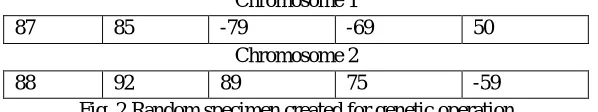
A randomly generated initial chromosome is created by keeping stocks at the lower and upper limits for all participants in the blood supply chain, plants, and distribution centers. As we know, the chromosome consists of genes that determine the length of the chromosomes. The inventory of each member of the chromosome is called the chromosome gene. A randomly generated initial chromosome is created by keeping stocks at the lower and upper limits for all participants in the blood supply chain, plants, and distribution centers. As we know, the chromosome consists of genes that determine the length of the chromosomes. The inventory of each member of the chromosome is called the chromosome gene.
Chromosome 1
87 85 -79 -69 50 Chromosome 2
[image:6.612.158.457.524.580.2]88 92 89 75 -59 Fig. 2 Random specimen created for genetic operation
These types of chromosomes are produced for genetic surgery. Initially, only two chromosomes are generated, and one random chromosome value is generated from the next generation. The resulting chromosomes are then used to determine the number of entries in the database contents using the select count () function. The function indicates the number of occurrences / repetitions of the corresponding inventory for ten items that will continue to be used in the format function.
B. Selection
439
©IJRASET: All Rights are Reserved
C. Fitness
Formatting functions ensure that evolution proceeds to optimization by calculating the form value for each person in the population. A fitness score assesses each person’s performance in a population.
U(i) = i= 1,2,3,4,5,6,7LL, n
Where, MP is the number of counts that occurs throughout the period. Mq is the total number of inventory values obtained after clustering.
n is the total number of chromosomes for which the fitness function is calculated.
A fitness function is performed for each chromosome, and the chromosomes are sorted according to the result of the fitness function. Subsequently, the chromosomes of the genetic operation are crossed and mutated.
D. Crossover
In this study, the intersection operation uses the intersection operator of one point. The first two chromosomes in the marriage pool are selected for the operation of crossing. The intersection operation performed for the sample case is shown in Figure 3 below.
Before Crossover
87 79 -69 68 78 86 -76 -68 71 81
After Crossover
[image:7.612.159.453.280.411.2]96 91 57 -41 70 -90 86 -70 74 72
Fig.3. Chromosome representation
The genes on the right side of the intersection point in both chromosomes are exchanged, and a crossing operation takes place. After the operation, two new chromosomes are obtained.
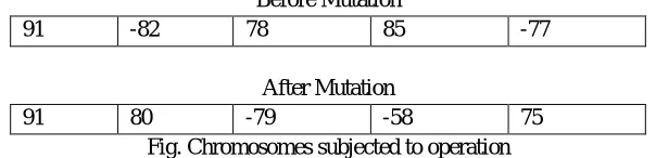
E. Mutation
Newly acquired chromosomes during a crossing operation are forced to mutate. A mutation creates a new chromosome (see Image below).
Before Mutation
91 -82 78 85 -77 After Mutation
91 80 -79 -58 75 Fig. Chromosomes subjected to operation This is done by randomly generating two points and then exchanging between both genes.
[image:7.612.155.457.509.582.2]440
©IJRASET: All Rights are Reserved
VI. NUMERICAL ILLUSTRATION
To illustrate the model numerically the following parameter values are considered.
0
(
u
2)
= 220 units,
EC OC= Rs. 220 per order,
r
0
3
2
= 2.25 unit,(
0
1
2)
= 0.24 unit,
ECHC= Rs. 20.10 per unit, θ =0.204 unit,t
1= 0.24 year,
EC LS= Rs. 8.20 per unit,
δ
0
2
2
= 0.22 unit, T = 2 year,Then for the minimization of total average cost and with help of software. the optimal policy can be obtained such as:
2
t
= 2.99 year, S = 276.8991 units and E.C.D.C.T.C.= Rs.2326.28 per year.Comparison of the optimization methods GA to enhance Electronic Components Distribution centre Inventory in presence of FACTS device is presented in this section. The control parameter values for all the optimization algorithms are given below GA: real coded,
Population=60 Generations=600
Crossover probability=1.0 Mutation probability=0.2
VII. SENSITIVITY ANALYSIS
Table:-1 Effect on optimal solution for distinct values of demand parameter
(
u
0
2)
% change in
(
u
0
2)
(
u
0
2)
TTCECDC
-20 252.5 282.65 2250.53 -15 254 282.57 2249.35 0 256.7 282.55 2248.23 15 258 282.85 2248.00 20 250.2 282.75 2247.98
Table:-2 Effect on optimal solution for distinct values of demand parameter
(
0
1
2)
% change in
(
0
1
2)
(
0
1
2)
TTCECDC
-20 20.62 232.65 2380.53 -15 20.62 232.57 2379.35 0 20.7 232.55 2368.23 15 20.72 231.85 2358.00 20 20.72 231.75 2347.98Table:-3 Effect on optimal solution for distinct values of backlogging parameter
δ
0
2
2
% change in
δ
0
2
2
δ
0
2
2
TTCBBS
441
©IJRASET: All Rights are Reserved
Table:-4 Effect on optimal solution for distinct values of selling price (
BB LS) % change in
EC LS
EC LS TTCECDC
-20 224.5 252.65 2478.53 -15 224.9 252.57 2477.35 0 225.0 252.55 2476.23 15 225.2 252.85 2476.20 20 225.9 252.75 2475.98Table:-5 Effect on optimal solution for distinct values of deterioration parameter
θ
2
2
% change in
θ
2
2
θ
2
2
TTCECDC
-20 20.00 272.65 2308.53 -15 20.62 272.57 2307.35 0 20.7 272.55 2306.23 15 20.72 270.85 2306.00 20 20.74 270.75 2305.98
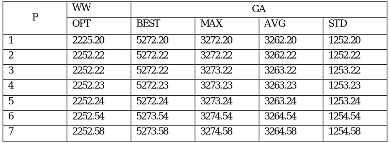
Optimization of control Electronic Components Distribution centre inventory in Electronic Components Distribution centre supply chain management using genetic algorithms is analyzed using MATLAB. Inventory levels for three different participants in the Electronic Components Distribution centre supply chain, ordering cost, holding cost, Deterioration cost, shortage cost and lost sales cost are created using the MATLAB script. This generated data set is used to evaluate the performance of a genetic algorithm. Some examples of the data sets used in the implementation are listed in Table 6. Table 6 lists about 5 records that are assumed to be records for the past period.
Table 6.: - Lists about 5 records that are assumed to be records for the past period S.N. Ordering cost Holding cost Deterioration
cost
Shortage cost
[image:9.612.105.507.574.722.2]lost sales cost 1 66 15 46 -49 66 2 -70 25 47 56 66 3 74 35 -55 58 66 4 75 -45 57 62 66 5 -79 46 -60 53 -51
Table: -7 Genetic Algorithm (GA) model optimal solution P
WW GA
442
©IJRASET: All Rights are Reserved
VIII. OBSERVATIONS
A. Table 1 shows the effect of demand parameter
(
u
0
2)
on T and onTCECDC
from this, we have noticed that an increase in demand parameter(
u
0
2)
shows a reverse effect of decrement in T and the same effect of increment inTCECDC
B. Table 2 presents the effect of demand parameter
(
0
1
2)
on T and onTCECDC
It is noticed that with an increment in demand parameter(
0
1
2)
, values of ‘T’ increase while value ofTCECDC
decreases.C. Table 3 presents the deviation of backlogging parameter
δ
0
2
2
at distinct points and it is noticed that as backlogging parameter
δ
0
2
2
increases, the values of T andTCECDC
decrease.D. Table 4 lists the variation in selling price
EC LS and from this; we have noticed that an increment in selling price shows maintains a reverse effect of decrement inTCECDC
.E. Table 5 shows the deviation of deterioration parameter
θ
2
2
at distinct points and it is noticed that as deterioration parameter
θ
2
2
increases, the values of and ‘T’ decrease whileTCECDC
increases.IX. CONCLUSION
This study incorporates some realistic features that are likely to be associated with the Electronic Components Distribution centre inventory of any material using Genetic Algorithm. Decay (deterioration) overtime for any material product and occurrence of shortages in inventory are natural phenomenon in real situations using Genetic Algorithm. Electronic Components Distribution centre Inventory shortages are allowed in the model using Genetic Algorithm. In many cases customers are conditioned to a shipping delay, and may be willing to wait for a short time in order to get their first choice using Genetic Algorithm. Generally speaking, the length of the waiting time for the next replenishment is the main factor for deciding whether the backlogging will be accepted or not using Genetic Algorithm.
The willingness of a customer to wait for backlogging during a shortage period declines with the length of the waiting time using Genetic Algorithm.
Thus, Electronic Components Distribution centre inventory shortages are allowed and partially backordered in the present chapter and the backlogging rate is considered as a decreasing function of the waiting time for the next replenishment using Genetic Algorithm. Demand rate is taken as exponential ramp type function of time, in which demand decreases exponentially for some initial period and becomes steady later on using Genetic Algorithm. Since most decision makers think that the inflation does not have significant influence on the inventory policy, the effects of inflation are not considered in some inventory models. However, from a financial point of view, an inventory represents a capital investment and must complete with other assets for a firm’s limited capital funds using Genetic Algorithm.
Thus, it is necessary to consider the effects of inflation on the inventory system. Therefore, this concept is also taken in this model. From the numerical illustration of the model, it is observed that the period in which inventory holds increases with the increment in backlogging and ramp parameters while inventory period decreases with the increment in deterioration and inflation parameters. Initial inventory level decreases with the increment in deterioration, inflation and ramp parameters while inventory level increases with the increment in backlogging parameter using Genetic Algorithm.
443
©IJRASET: All Rights are Reserved
REFERENCES
[1] Yadav, A.S. and Swami, A. (2018) Integrated Supply Chain Model For Deteriorating Items With Linear Stock Dependent Demand Under Imprecise And Inflationary Environment. International Journal Procurement Management, Volume 11 No 6.
[2] Yadav, A.S. and Swami, A. (2018) A partial backlogging production-inventory lot-size model with time-varying holding cost and weibull deterioration International Journal Procurement Management, Volume 11, No. 5.
[3] Yadav, A.S., Swami, A. and Kumar, S. (2018) A supply chain Inventory Model for decaying Items with Two Ware-House and Partial ordering under Inflation. International Journal of Pure and Applied Mathematics, Volume 120 No 6.
[4] Yadav, A.S., Swami, A. and Kumar, S. (2018) An Inventory Model for Deteriorating Items with Two warehouses and variable holding Cost International Journal of Pure and Applied Mathematics, Volume 120 No 6.
[5] Yadav, A.S., Swami, A. and Kumar, S. (2018) Inventory of Electronic components model for deteriorating items with warehousing using Genetic Algorithm. International Journal of Pure and Applied Mathematics, Volume 119 No. 16.
[6] Yadav, A.S., Johri, M., Singh, J. and Uppal, S. (2018) Analysis of Green Supply Chain Inventory Management for Warehouse With Environmental Collaboration and Sustainability Performance Using Genetic Algorithm. International Journal of Pure and Applied Mathematics, Volume 118 No. 20. [7] Yadav, A.S., and Kumar, S. (2017) Electronic Components Supply Chain Management for Warehouse with Environmental Collaboration & Neural Networks.
International Journal of Pure and Applied Mathematics, Volume 117 No. 17.
[8] Yadav, A.S., Taygi, B., Sharma, S. and Swami, A. (2017) Effect of inflation on a two-warehouse inventory model for deteriorating items with time varying demand and shortages International Journal Procurement Management, Volume 10, No. 6.
[9] Yadav, A.S., Mahapatra, R.P., Sharma, S. and Swami, A. (2017) An Inflationary Inventory Model for Deteriorating items under Two Storage Systems International Journal of Economic Research, Volume 14 No.9.
[10] Yadav, A.S., Sharma, S. and Swami, A. (2017) A Fuzzy Based Two-Warehouse Inventory Model For Non instantaneous Deteriorating Items With Conditionally Permissible Delay In Payment, International Journal of Control Theory And Applications, Volume 10 No.11.
[11] Yadav, A.S., (2017) Analysis Of Supply Chain Management In Inventory Optimization For Warehouse With Logistics Using Genetic Algorithm International Journal of Control Theory And Applications, Volume 10 No.10.
[12] Yadav, A.S., Swami, A., Kher, G. and Kumar, S. (2017) Supply Chain Inventory Model for Two Warehouses with Soft Computing Optimization International Journal of Applied Business and Economic Research Volume 15 No 4.
[13] Yadav, A.S., Mishra, R., Kumar, S. and Yadav, S. (2016) Multi Objective Optimization for Electronic Component Inventory Model & Deteriorating Items with Two-warehouse using Genetic Algorithm International Journal of Control Theory and applications, Volume 9 No.2.