Online Full Text

Abstract— Species richness is one of the important measures used by ecologists. In this paper we try to predict the changes in the number of species and to identify the most important features that can be used. For this reason we used EcoSim a multi-food chain evolving ecosystem simulation. In this study we predict the variations in the number of species in EcoSim by applying machine learning techniques. We show that environmental and genetic factors have a critical role in this prediction. Identifying important features for species richness prediction and the relationship between them could be beneficial for future conservation studies.

Index Terms— ecosystem simulation, decision tree, prediction, species richness

I. INTRODUCTION

PECIES richness is a critical variable for biodiversity management that has been used for decision making and prioritization of conservation efforts [1-3]. Ecological theory assumes that species richness is determined in part by environmental gradients and resources [4]. Defining a set of environmental variables which are recognized to entail direct or indirect responses from presence/absence species and linking them by an ecologically-relevant statistical model enable the acquisition of significant information aimed at conservation planning [4-7]. Several studies have also demonstrated strong relationships between total species richness and measures of temperature, precipitation and net primary productivity [8-12]. Developing a standardized method of predicting species richness is vital for international conservation efforts [1-3], [13]. Few tools are available to provide decision makers with relevant data on biodiversity patterns, ecosystem processes, and underlying forces at spatial scales from local to global [14].

Considering working with real data, it is highly expensive and time-consuming to measure species richness over extensive areas, especially for nonvascular plants and invertebrates and in tropical or marine ecosystems [15-16].

Manuscript received July 09, 2012; revised August 06, 2012. This work was supported by the NSERC grant ORGPIN 341854, the CRC grant 950-2- 3617 and the CFI grant 203617 and is made possible by the facilities of the Shared Hierarchical Academic Research Computing Network.

Abbas Golestani is with the School of Computer Science, University of Windsor, ON N9B3P4 Canada (e-mail: [email protected]).

Robin Gras is with the School of Computer Science and Department of Biology, University of Windsor, ON N9B3P4 Canada (e-mail: [email protected]).

By using computer simulations, it would be possible to examine factors that could affect the performance of models that predict species occurrence based on environmental variables [17]. Simulation modeling explicitly incorporates the processes believed to be affecting the geographical ranges of species and generates a number of quantitative predictions that can be compared to empirical patterns. The simulation approach offers new insights into the origin and maintenance of species richness patterns, and may provide a common framework for investigating the effects of contemporary climate, evolutionary history and geometric constraints on global biodiversity gradients [18]. But most of the simulations failed to provide a conceptual bridge between macroecology and biogeography. The problem is that those simulations are contain a lots of simplifications [18]. They are not as complex as real ecosystems [19, 22], therefore in most cases the results that come from those simulations are not anymore valid for making any conclusion for real systems.

In this research, we try to predict the changes in the number of species using several of important features by applying machine learning techniques such as different feature selection algorithms and decision tree. To best of our knowledge, this is the first time that a complex agent-based simulation (EcoSim [23]) has been used to examine the effects of different features on prediction of changes in species richness by extracting meaningful rules from environmental and genetic parameters. Several studies evaluated the capacity of the EcoSim platform to model real ecosystems and to make realistic predictions regarding species abundance patterns [20] and the complexity levels of the simulation [21]. These studies show that the communities of species generated by the simulation follow the same lognormal law as natural communities and that EcoSim can help evaluate the overall level of diversity of a given community.

For extracting rules and finding a relationship between environmental variables and species richness, different approaches using nonparametric coefficients, especially decision trees, have been demonstrated to outperform linear models since both linear and nonlinear relationships between biotic and abiotic components were well identified [24]. Therefore we used this machine learning algorithm to select potential features for the sake of species richness prediction. Our objective in this study, was to conduct a robust test of

S

Using Machine Learning Techniques for

Identifying Important Characteristics to Predict

Changes in Species Richness in EcoSim, an

Individual-Based Ecosystem Simulation

the effectiveness of our framework for identifying important features in prediction of changes in the number of species and introducing a restricted set of features that could help biologists to focus on a specific variables (since there are lots of features that can be studied by biologists). Using these simulations as a shortcut can save time and resources for biologists. Besides, the relationships between these features that can be discovered in the predictive rules extracted by our approach could lead to a good combination of features that biologists can use it in their future studies.

This paper is organized as follows: In section II, we present our ecosystem simulation. In section III, we explain the details of methodologies for computation and selection of important features and then we present the obtained results from applying prediction method to the species richness of ecosystem simulation.

II. AN INDIVIDUAL-BASED ECOSYSTEM SIMULATION In this section, the main parts of the evolving agent-based predator/prey ecosystem EcoSim are briefly introduced. The comprehensive description of this simulation has been proposed in [23]. This simulation is a logical description of how a simple ecosystem performs. In this simulation, complex adaptive agents (individuals), each one of them using a Fuzzy Cognitive Map (FCM) as a behavioral model, are either a prey or a predator and a virtual torus world is implemented as a 1000 × 1000 matrix of cells.

A. Fuzzy Cognitive Maps

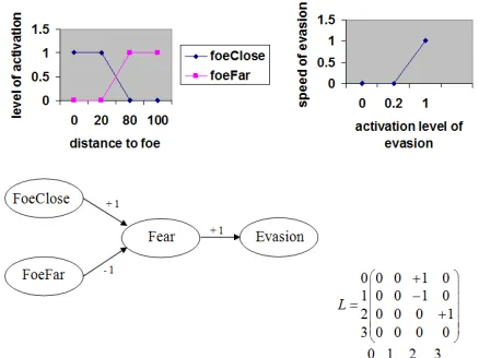
FCMs are weighted graphs aiming to represent the causal relationship between concepts and to analyze inference patterns. In our simulation, the FCM is not only the base for describing and computing the agent behaviors, but also the platform for modeling the evolutionary mechanism and the speciation events as it is coded in the individual’s genome. Each individual performs an action during a time step based on its perception of the environment. The FCM, called a map in our system, is used to model the agent behaviors (structure of the graph) and to compute the next action of the agent (dynamics of the map). A map contains three kinds of concepts: sensitive, internal, and motor. The activation level of a sensitive concept is computed by a fuzzification of the information coming from the environment (see Fig. 1). The activation level of the motor concept is used to determine what the next action of the agent will be, and a defuzzification of its value can be used to determine the amplitude of the action. Finally, the internal concepts' activation levels correspond to the levels of intensity of the internal states of the agent and affect the computation of the dynamic of the map.

B. Intelligent Agents

Each agent has one FCM and several properties that determine its physical capabilities and its behaviors. The behaviors are determined by the interaction between the FCM and the environment. Each agent possesses its own FCM (coded in its genome, which is subject of the evolutionary process). The FCM contains sensitive concepts like foeClose, foodClose, energyLow, internal concepts like fear, hunger, curiosity, satisfaction, and motor concepts like evasion, socialization, exploration, and breeding. It also contains links and weights representing the mutual influences

between these concepts. The FCM of an agent, coded in its genome, is transmitted to its offspring after being combined with the one of the other parent and after the possible addition of some mutations. The behavior model of each agent is therefore, unique.

As an example, a very simple map can be defined to model an agent perceiving and reacting to its distance from a foe. The closer the foe, the more frightened the agent. Depending on this distance and also on the fear level, the agent will decide whether or not it will evade. The more frightened the agent, the faster the evasion. An FCM corresponding to this example is given in Fig. 1. In this example, there are two sensitive concepts: foeClose and

foeFar, one internal: fear and one motor: evasion. There are

also three influence edges: closeness to a foe excites fear, distance to a foe inhibits fear and fear causes evasion. Activations of the concepts foeClose and foeFar are computed by fuzzyfication of the real value of the distance to the foe, and the defuzzyfication of the activation of evasion tells us about the speed of the evasion. In our simulation each individual posses its proper map which contains around 30 concepts and hundreds of edges.

C. Species

Fig. 1. A simple fuzzy cognitive map for detection of foe and decision to evade with its corresponding matrix with 0 for “Foe close”, 1 for “Foe far”, 2 for “Fear” and 3 for “Evasion” and the fuzzyfication and defuzzyfication

functions.

D. Update

At each time step, the values of the states of all the parameters in the model are updated. The successive phases of the update process are as follows for each agent: perception of the environment, computation of all concepts of its map, application of their selected action and update of the energy level. Then, there is an update of the lists of agents, species and cells around the world. For each action which requires the agent movement, its speed is proportional to the level of activation of the corresponding action concept. Fig. 2 shows the population of prey and predator agents after each time step. These patterns and the properties of the communities of species that are generated by simulation have been shown to be very similar to the ones observed for real communities of species [20]. A recent execution of the simulation produced approximately 30,000 time steps in 60 days by using the SHARCNET resources. The computed average and standard deviation for the number of prey individuals are 150,000 and 47,000 respectively (for predator 21,000 and 8,000) and the average and standard deviation for the number of prey species are 22 and 7 (for predator 13 and 4).

Fig. 2. Population of prey and predator agents.

III. RESULTS

A. Development of a predictive model

In this study, the goal is the prediction of changes in species richness 100 time steps later using a set of features from EcoSim which produces a large amount of data about

the individuals and the species in each time step. We conducted three runs of the simulation with the same parameters. The prepared training dataset comes from two independent runs that contain 20,000 samples (10000 time steps for each unique run) related to about 38 species in average. Each sample is label ‘smaller’ or ‘bigger’ if the number of species in the world respectively has decreased or has increased (or without change) 100 time steps later. The test set contains about 10,000 samples. Both the training and the test datasets contains almost an equal number of 'smaller' labels and 'bigger' labels. The most important part for prediction is the selection of the most significant features. In each time step, every individual has a certain number of attributes (feature). We started our learning process with an initial set of 49 features. These features are average over all individuals and are: 12 sensitive concepts’ average activation level, 7 internal concepts’ average activation level, 7 motor concepts’ average activation level, 11 actions frequency, the total amount of food in the world, the total population size, the ratio of individuals in a species to the whole population size, the number of dead individuals in the world, the genetic diversity of the whole population, the average age of individuals, the average energy and speed of individuals, the average genetic distance of all the genomes of the individuals from initial genome, the average amount of energy transmit from a parent to a child (parental investment) and the current number of species. The genetic diversity of a species measures how much diversity exists in the gene pool of the individuals of a species. The entropy measure, which we use in this project, is commonly used as an index of diversity in ecology and increasingly used in genetics [26].

order to get a smaller tree for extracting meaningful rules with reasonable accuracy, we chose to use decision tree with the confidence factor 0.25 for pruning and 100 minimum instances per leaf [27]. This ensured that the final model neither fitted too specific of the training data set, nor was so general that it renders its predictions meaningless. With this reduction in size, the obtained tree has 10 rules (Fig. 3). The accuracy decreased by 7% on training set and increased by 3% accuracy on validation set.

For comparing the quality of classification, four measures of accuracy, true positive (TP) rate, true negative (TN) rate, global accuracy, and ROC area have been used. The global accuracy shows the percentage of correctly classified samples. The true positive (negative) rate presents the percentage of true classified positive (negative) samples. Finally, ROC area reveals sensitivity by measuring the fraction of true positives out of the positives versus the fraction of false positives out of the negatives.

For the training and test set, using 10-fold cross-validation, the final tree model has a total accuracy of 82%, the two classes being predicted with almost the same high accuracy. The accuracy of the prediction on training data sets with 10-fold cross-validation is given shown in TABLE I.

TABLE I. Results of prediction on train set. Class TP Rate FP Rate Precision ROC Area

Smaller 0.834 0.184 0.794 0.89

Bigger 0.816 0.166 0.853 0.89

Total 0.824 0.174 0.826 0.89

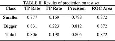
For the test set, we picked a completely separate run of simulation. In this case the total accuracy is about 80% which means that, using selected features, prediction of changes in species richness time series is possible with high level of accuracy even on data generated by an independent process (TABLE II). This means that the rules we have discovered all quite general and could bring some interesting insight on the speciation process.

TABLE II. Results of prediction on test set. Class TP Rate FP Rate Precision ROC Area

Smaller 0.777 0.169 0.798 0.872

Bigger 0.831 0.223 0.812 0.872

Total 0.806 0.198 0.805 0.872

B. Extracting the Rules from Decision Tree

Decision tree effectively modeled much of the variations in species richness as this method was able to both select a relevant set of predictor variables and to make accurate predictions. The splitting rules used in the partitioning algorithm split the data at values that were ecologically meaningful, describing the relationship between species richness and environmental parameters. This demonstrates the utility of trees as a powerful exploratory modeling tool for building and analyzing prediction models in ecology.

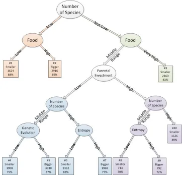
Looking at the selected features and the tree obtained for prediction (Fig. 3), we can conclude that genetic features and world productivity have an important role on variation of species richness. We can also observe that the tree is well

balanced in term of rule support and in term of accuracy. It means that all of the rules are important and correspond to a situation characteristic of one of the two possible states we try to predict. One of the rules is about a very high amount of food availability and the number of species that is not low (Rule #3). This rule associates the high level of food to a decrease in the number of species. According to several studies [28, 29], this rule makes sense because when there is a high amount of food in the environment means there is few individuals that consume it. Low number of individuals could be a sign for a low number of species. According to [28], richness of animal populations is determined by the abundance, distribution and diversity of food resources.

If the number of species is low and also the amount of available food is low (Rule #1), it should means that the environment is particularly difficult, the fact that it leads to a decrease in the number of species is quite intuitive. However, this rule is the one with the lowest accuracy which mean that the phenomenon is not as simple as that. This should explain the multiple rules that exist (#4 to #10) that are in the ‘Middle Range’ for the amount of food available. If the amount of food is high (Rule #2), it means that it is easy for the individuals to survive and reproduce and, with an increase in population size and as the number of species is currently low, we can expect an increase in the number of species. Using machine learning algorithms like the one that we used allows discovering how adjusting amount of food can be used to control the system. This mechanism could be a direction for future conservation researches.

These two cases correspond to extreme situations for the availability of food, but there are intermediate situations. These cases are trickier for prediction and need the use of other features. Our model discovers the interest of the variable describing parental investment (the average amount of energy transmit from a parent to a child). When parental investment is low and the number of species is also low, the variable describing the distance evolution become involved. Distance evolution reflects the genetic evolution of individuals from beginning. If distance evolution is high (Rule #5), which represent situation in which the evolution is fast, the possibility of an increase in number of species arises and we could expect an increase in the number of species. This rule is one of the most important one, with the highest support and a very good accuracy.

Fig. 3. The decision tree corresponding to the partitioned feature space for prediction of changes in species richness. Number of samples covered by each rule and the accuracy are also given.

This process also was found by [30], which shows speciation through an increase in genetic variance between populations can occur by evolution over time. This phenomenon has also already been observed in EcoSim [31].

When the parental investment is high and the average number of species are in a middle range, the next important feature again is genetic diversity. High value of genetic diversity (Rule #9) could stand for more possibility of speciation in the next time steps for the same reasons that have been explained above and for low genetic diversity (Rule #8), number of species decreases as well. The parental investment feature itself stands for the amount of energy that is transferred from parents to the new-born individuals. This feature is also subject to mutation during evolutionary process. High value of parental investment and high number of species (Rule #10, which has the highest accuracy and a good support) means that for such situation (there is also not much food available) having a high parental investment in energy to their child leads to a high probable decrease in the number of species. Other studies also emphasize the effect of balance of energy on species richness [32]. Environmental energy availability can explain much of the spatial variation in species richness [33 - 35].

By identifying the most influential variables (and the relative value for each feature that leads to specific rule), this study provides an important first step towards the

development of future predictions of species richness for predator-prey ecosystems that can incorporate higher resolution data.

IV. CONCLUSION

In this paper a machine learning techniques has been applied to data generated by EcoSim, an individual-based ecosystem simulation, to predict variations in species richness. Our objective in this study, was to conduct a robust test of the effectiveness of our framework for identifying important features for species richness prediction. We initially used all possible features available to predict species richness. Then we used feature selection algorithms such as Greedy-Stepwise and Linear-Forward-Selection to detect the five most important features that guarantee maximum possible prediction accuracy. By interpreting the obtained decision tree we have been able to extract meaningful rules to enrich our knowledge about the kind of features involved and how their combination can be used to predict species richness variation.

whole concept of species rely on the notion of similar genetic characteristics. These results confirmed, that our implementation of species in EcoSim has the capacity to reflect concepts and behaviors observed in population genetics that affect the species richness of an ecosystem.

REFERENCES

[1] Environment Conservation Council (Victoria). Box-ironbark forest and woodlands investigation. EEC. Melbourne, Australia, 2000. [2] S.L. Pimm, et al. Can we defy nature's end? Science, vol. 293, pp.

2207-2208, 2001.

[3] C.M. Roberts, et al. Marine biodiversity hotspots and conservation priorities for tropical reefs. Science, vol 295, 2002, pp. 1280-1284. [4] M.P. Austin, Species distribution models and ecological theory: A

critical assessment and some possible new approaches. Ecological Modeling, vol. 200, pp. 1-19, 2007.

[5] A. Guisan, N.E. Zimmermann, Predictive habitat distribution models in ecology. Ecological Modeling, vol. 135, pp. 147–186, 2000. [6] M.P. Austin, Spatial prediction of species distribution: an interface

between ecological theory and statistical modeling. Ecological Modeling, vol. 157, pp. 101–118, 2002.

[7] A. Collin, P. Archambault, B. Long, Predicting species diversity of benthic communities within turbid nearshore using full-waveform bathymetric LiDAR and machine learners. PLoS ONE, vol. 6, pp. e21265, 2011.

[8] D.J. Currie, Energy and large-scale patterns of animal species and plant-species richness. Am. Nat., vol. 137, pp. 27–49, 1991. [9] C. Rahbek, and G.R. Graves, Multiscale assessment of patterns of

avian species richness. Proc. Natl Acad. Sci., vol. 98, vol. 4534-4539, 2001.

[10] B.A. Hawkins, et al. Energy, water, and broad-scale geographic patterns of species richness. Ecology vol. 84, pp. 3105–3117, 2003. [11] D.J. Currie, et al. Predictions and tests of climate-based hypotheses of

broad-scale variation in taxonomic richness. Ecol. Lett. Vol. 7, pp.1121–1134, 2004.

[12] C. Rahbek, et al. Predicting continental-scale patterns of bird species richness with spatially explicit models. – Proc. R. Soc. B, vol. 274, pp.165-174, 2007.

[13] R.M. Nally, and E. Fleishman, A successful predictive model of species richness based on indicator species. Conserv. Biol., vol. 18, pp. 646–654, 2004.

[14] V. Gewin, The state of the planet. Nature , vol. 417, pp. 112-113, 2002.

[15] R.L. Pressey, T.C. Hager, K.M. Ryan, J. Schwarz, S. Wall, S. Ferrier, P.M. Creaser, Using abiotic data for conservation assessments over extensive regions: quantitative methods applied across New South Wales, , Biological Conservation, vol. 96, pp. 55-82, 2000.

[16] D.P. Faith, et al. The BioRap biodiversity assessment and planning study for Papua New Guinea. Pacific Conservation Biology vol. 6, pp. 279-288, 2001.

[17] G.C. Reese, et al. Factors affecting species distribution predictions: a simulation modeling experiment. Ecol. Appl. vol. 15, pp. 554–564, 2005.

[18] N. Gotelli, et al.(2009) Patterns and causes of species richness: A general simulation model for macroecology. Ecol Lett, vol. 12, pp. 873–886, 2009.

[19] A. Golestani, and R. Gras, Regularity Analysis of an individual-based Ecosystem Simulation, Chaos, vol. 20, pp. 043120. 1-13, 2010. [20] D. Devaurs and R. Gras, “Species abundance patterns in an ecosystem

simulation studied through Fisher’s logseries,” Simulation Modelling Practice and Theory, vol. 18, pp. 100-123, 2010.

[21] Y.M. Farahani, A. Golestani and R. Gras, Complexity and Chaos Analysis of a Predator-Prey Ecosystem Simulation, COGNITIVE '10, 2010, pp. 52-59.

[22] L. Romanelli, M.A. Figliola, and F.A. Hirsch, Deterministic Chaos and Natural Phenomena. J. Stat. Phys. vol. 53, pp. 991-994, 1988. [23] R. Gras, D. Devaurs, A. Wozniak, and A. Aspinall, An

individual-based evolving predator-prey ecosystem simulation using a fuzzy cognitive map as the behavior model. Artificial life, vol. 15, pp. 423-463, 2009.

[24] S.J. Pittman, J.D. Christensen, C. Caldow, C. Menza and M.E. Monaco, Predictive mapping of fish species richness across

shallow-water seascapes in the Caribbean. Ecological Modelling vol. 204, pp. 9–21, 2007.

[25] A. Aspinall, and R. Gras, K-means clustering as a speciation mechanism within an individual-based evolving predator-prey ecosystem simulation. Active Media Technology, pp. 318-329, 2010. [26] W.B. Sherwin,. Entropy and Information Approaches to Genetic

Diversity and its Expression: Genomic Geography. Entropy, vol. 12, pp. 1765-1798, 2010.

[27] J.R. Quinlan, C4. 5: programs for machine learning. Morgan Kaufmann, 1993.

[28] W.D. Kissling, C. Rahbek, and K. Böhning-Gaese, ( Food plant diversity as broad-scale determinant of avian frugivore richness. Proceedings of the Royal Society B, vol. 274, pp. 799–808, 2007. [29] D. Oro, E. Cam, R. Pradel, and A. Martinez-Abrain, Influence of food

availability on demography and local population dynamics in a long-lived seabird. Proceedings of the Royal Society of London vol. 271, pp. 387–396, 2004.

[30] C. Devaux and R. Lande, Incipient allochronic speciation due to non-selective assortative mating by flowering time, mutation and genetic drift. Proc. R. Soc. B. vol. 275, pp. 2723–2732, 2008.

[31] A. Golestani, R. Gras, and M. Cristescu, Speciation with gene flow in a heterogeneous virtual world: can physical obstacles accelerate speciation?, Proc. R. Soc. B, vol. 279 no. 1740, 2012, pp 3055-3064, 2012.

[32] K.L. Evans, J.J.D. Greenwood, K.J. Gaston, Dissecting the species-energy relationship. Proc. R. Soc. B, vol. 272, pp. 2155–2163, 2005. [33] D.J. Currie, Energy and large-scale patterns of animal and plant

species richness. Am. Nat. vol. 137, pp. 27–49, 1991.

[34] K. Roy, D. Jablonski, J.W. Valentine, and G. Rosenberg, Marine latitudinal diversity gradients: tests of causal hypotheses. Proc. Natl Acad. Sci. vol. 95, pp. 3699–3702, 1998.

[35] J.A. Crame, Taxonomic diversity gradients through geological time. Divers. Distrib. vol. 7, pp. 175–189, 2001.