Semiring Parsing

J o s h u a G o o d m a n * Microsoft Research

We synthesize work on parsing algorithms, deductive parsing, and the theory of algebra applied

to formal languages into a general system for describing parsers. Each parser performs abstract

computations using the operations of a semiring. The system allows a single, simple representation

to be used for describing parsers that compute recognition, derivation forests, Viterbi, n-best,

inside values, and other values, simply by substituting the operations of different semirings. We

also show how to use the same representation, interpreted differently, to compute outside values.

The system can be used to describe a wide variety of parsers, including Earley's algorithm, tree

adjoining grammar parsing, Graham Harrison Ruzzo parsing, and prefix value computation.

1. I n t r o d u c t i o n

For a given grammar and string, there are m a n y interesting quantities we can compute. We can determine whether the string is generated by the grammar; we can enumerate all of the derivations of the string; if the grammar is probabilistic, we can compute the inside and outside probabilities of components of the string. Traditionally, a different parser description has been needed to compute each of these values. For some parsers, such as CKY parsers, all of these algorithms (except for the outside parser) strongly resemble each other. For other parsers, such as Earley parsers, the algorithms for computing each value are somewhat different, and a fair amount of work can be required to construct each one. We present a formalism for describing parsers such that a single simple description can be used to generate parsers that compute all of these quantities and others. This will be especially useful for finding parsers for outside values, and for parsers that can handle general grammars, like Earley-style parsers.

Although our description format is not limited to context-free grammars (CFGs), we will begin by considering parsers for this common formalism. The input string will be denoted wlw2... Wn. We will refer to the complete string as the sentence. A CFG G is a 4-tuple (N, ~, R, S) where N is the set of nonterminals including the start symbol S, ~ is the set of terminal symbols, and R is the set of rules, each of the form A --* a for A c N and a E (N U ~)*. We will use the symbol ~ for immediate derivation and

for its reflexive, transitive closure.

We will illustrate the similarity of parsers for computing different values using the CKY algorithm as an example. We can write this algorithm in its iterative form as shown in Figure 1. Here, we explicitly construct a Boolean chart,

chart[1..n, 1..IN I,

1..n + 1]. Element chart[i,A,j] contains

TRUE

if and only if A G w i . . . wj-1. The algo- rithm consists of a first set of loops to handle the singleton productions, a second set of loops to handle the binary productions, and a return of the start symbol's chart entry. Next, we consider probabilistic grammars, in which we associate a probability with every rule,

P(A --* a).

These probabilities can be used to associate a probability

Computational Linguistics Volume 25, Number 4

boolean chart[1..n, 1..IN I, 1..n+1] := FALSE;

for s := 1 to n / * start position */

for each rule A -+ ws c R chart[s, A, s + l ] := TRUE;

for l := 2 to n / * length, shortest to longest */

for s := 1 to n - l + 1 / * s t a r t p o s i t i o n */

for t := 1 to / - 1/* split length */

for each rule A -+ B C ¢ R

/* extra TRUE for expository purposes */ chart[s, A, s.l.l] := chart[s, A, s+l] V

(chart[s, B, s + t] A chart[s ÷ t, C, s + l] A TRUE); r e t u r n chart[l, S, n + 1];

Figure 1

CKY recognition algorithm.

float chart[1..n, 1..IN[, 1..n÷1] := 0;

for s := I to n / * start position */

for each rule A --+ ws E R

chart[s, A, s + l ] := P ( A --+ ws);

for / := 2 to n / * length, shortest to longest */

for s := I to n - l + l /* start position */

for t := 1 to 1 - 1/* split length */

for each rule A -+ B C c R

chart[s, A, s+l] := chart[s, A, s+l] +

(chart[s, B, s+t] x chart[s+t, C, s+l] x P ( A -+ BC));

return chart[l, S, n+ 1];

Figure 2

CKY inside algorithm.

w i t h a particular derivation, equal to the p r o d u c t of the rule probabilities u s e d in the derivation, or to associate a probability w i t h a set of derivations, A ~ wi. • • wj-1 equal to the s u m of the probabilities of the i n d i v i d u a l derivations. We call this latter p r o b - ability the inside probability of i,A,j. We can rewrite the CKY a l g o r i t h m to c o m p u t e the inside probabilities, as s h o w n in Figure 2 (Baker 1979; Lari a n d Young 1990).

Notice h o w similar the inside algorithm is to the recognition algorithm: essentially, all that has b e e n d o n e is to substitute + for V, x for A, a n d P(A ~ ws) a n d P(A ~ BC) for TRUE. For m a n y parsing algorithms, this, or a similarly simple modification, is all that is n e e d e d to create a probabilistic version of the algorithm. O n the other h a n d , a simple substitution is not always sufficient. To give a trivial example, if in the CKY recognition algorithm w e h a d w r i t t e n

chart[s,A,s÷l] := chart[s,A,s÷l] V chart[s,B,s÷t] A chart[s+t,C,s÷l]; instead of the less natural

chart[s, A, s÷l] := chart[s,A, s,l,l] V chart[s, B, s+t] A chart[s+t, C, s-t-l] A TRUE; larger changes w o u l d be necessary to create the inside algorithm.

efficiently compute the set of legal derivations of the input string. The derivation for- est is typically found by modifying the recognition algorithm to keep track of "back pointers" for each cell of how it was produced. The second quantity often computed is the Viterbi score, the probability of the most probable derivation of the sentence. This can typically be computed by substituting x for A and max for V. Less commonly computed is the total number of parses of the sentence, which, like the inside values, can be computed using multiplication and addition; unlike for the inside values, the probabilities of the rules are not multiplied into the scores. There is one last commonly computed quantity, the outside probabilities, which we will describe later, in Section 4.

One of the key points of this paper is that all five of these commonly com- puted quantities can be described as elements of complete semirings (Kuich 1997). The relationship between grammars and semirings was discovered by Chomsky and Schiitzenberger (1963), and for parsing with the CKY algorithm, dates back to Teit- elbaum (1973). A complete semiring is a set of values over which a multiplicative operator and a commutative additive operator have been defined, and for which infi- nite summations are defined. For parsing algorithms satisfying certain conditions, the multiplicative and additive operations of any complete semiring can be used in place of A and V, and correct values will be returned. We will give a simple normal form for describing parsers, then precisely define complete semirings, and the conditions for correctness.

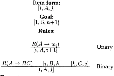
We now describe our normal form for parsers, which is very similar to that used by Shieber, Schabes, and Pereira (1995) and by Sikkel (1993). This work can be thought of as a generalization from their work in the Boolean semiring to semirings in general. In most parsers, there is at least one chart of some form. In our normal form, we will use a corresponding, equivalent concept, items. Rather than, for instance, a chart element chart[i,A,j], we will use an item [i,A,j]. Furthermore, rather than use explicit, procedural descriptions, such as

chart[s,A,s+l] := chart[s,A,s+l] V chart[s,B,s+t] A chart[s+t,C,s+l] A TRUE we will use inference rules such as

R(A ~ BC) [i,B,k] [k,C,j] [i,A,j]

The meaning of an inference rule is that if the top line is all true, then we can conclude the bottom line. For instance, this example inference rule can be read as saying that if A ~ BC and B G w i . . . Wk-1 and C ~ w k . . . wj-1, then A G w l . . . Wj_l.

The general form for an inference rule will be

A1 " . Ak B

where if the conditions A1 ... Ak are all true, then we infer that B is also true. The Ai can be either items, or (in an extension of the usual convention for inference rules) rules, such as R(A ~ BC). We write R(A ---* BC) rather than A --~ BC to indicate that we could be interested in a value associated with the rule, such as the probability of the rule if we were computing inside probabilities. If a n Ai is in the form R(...), we

call it a rule. All of the Ai must be rules or items; when we wish to refer to both rules and items, we use the word terms.

Computational Linguistics Volume 25, Number 4

Item form:

[i, A, j]

Goal:

[1, S, n + 1]

Rules:

R ( A -+ wi)

{i,A,i+l]

R ( A --+ BC)

[i, B, k]

[k, C, j]

[i, A, j]

Figure 3

Item-based description of a CKY parser.

Unary

Binary

semiring, w h o s e additive operator is addition a n d w h o s e multiplicative operator is multiplication. We use the input string

xxx

to the following grammar:

S ~

X X 1.0

X

--* X X

0.2 X --* x 0.8

(1)

Our first step is to use the u n a r y rule,

R(A

wi)

[i,A,i+l]

The effect of the u n a r y rule will exactly parallel the first set of loops in the CKY inside algorithm. We will instantiate the free variables of the u n a r y rule in every possible way. For instance, we instantiate the free variable i w i t h the value 1, a n d the free variable A w i t h the nonterminal X. Since wl = x, the instantiated rule is then

R(x

x)

[1,X,2]

Because the value of the top line of the instantiated u n a r y rule,

R(X ---,

x), has value 0.8, we deduce that the b o t t o m line, [1,X, 2], has value 0.8. We instantiate the rule in two other ways, a n d compute the following chart values:

[image:4.468.51.251.58.192.2]

[1,X,2] = 0.8 [2,X,3] = 0.8 [3,X,4] = 0.8

Next, w e will use the binary rule,

R(A --* BC)

[i, B, k] [k, C,j]

[i,A,j]

The effect of the binary rule will parallel the second set of loops for the CKY inside algorithm. Consider the instantiation i = 1, k -- 2, j = 3, A -- X, B = X, C -- X,

We use the multiplicative o p e r a t o r of the semiring of interest to m u l t i p l y together the values of the top line, d e d u c i n g that [1, X, 3] = 0.2 x 0.8 x 0.8 = 0.128. Similarly,

[image:5.468.149.304.189.255.2]

[1,X,3] = 0.128 [2,X,4] = 0.128 [1,S,3] -- 0.64 [2,S,4] = 0.64

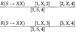
There are two m o r e w a y s to instantiate the conditions of the b i n a r y rule:

R(S --~ X X ) [1, X, 2] [2, X,4]

[1, S, 4]

R ( S --+ X X ) [1,X,3] [3, X,4] [1, S, 4]

The first has the v a l u e 1 x 0.8 x 0.128 = 0.1024, a n d the second also has the v a l u e 0.1024. W h e n there is m o r e than one w a y to derive a v a l u e for an item, w e use the additive o p e r a t o r of the semiring to s u m t h e m up. Thus, [1, S, 4] -- 0.2048. Since [1, S, 4] is the goal item for the CKY parser, w e k n o w that the inside v a l u e for xxx is 0.2048. The goal item exactly parallels the r e t u r n statement of the CKY inside algorithm.

1.1 Earley Parsing

M a n y parsers are m u c h m o r e complicated than the CKY parser, a n d w e will n e e d to e x p a n d o u r notation a bit to describe them. Earley's algorithm (Earley 1970) exhibits m o s t of the complexities w e wish to discuss. Earley's algorithm is often described as a b o t t o m - u p p a r s e r w i t h t o p - d o w n filtering. In a probabilistic f r a m e w o r k , the b o t t o m - u p sections c o m p u t e probabilities, while the t o p - d o w n filtering nonprobabilistically r e m o v e s items that cannot be derived. To capture these differences, w e e x p a n d o u r notation for d e d u c t i o n rules, to the following:

a l " " a k C 1 . . . C j B

C1 " " Cj are

side conditions,

i n t e r p r e t e d nonprobabilistically, while A1 .-- Ak are m a i n

conditions

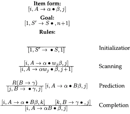
with values in w h i c h e v e r semiring w e are using. 1 While the values of all m a i n conditions are multiplied together to yield the v a l u e for the item u n d e r the line, the side conditions are i n t e r p r e t e d in a Boolean manner: if all of t h e m are n o n z e r o , the rule can be used, b u t if a n y of t h e m are zero, it c a n n o t be. O t h e r t h a n for checking w h e t h e r they are zero or n o n z e r o , their values are ignored.

Figure 4 gives an item-based description of Earley's parser. We a s s u m e the a d d i t i o n of a distinguished n o n t e r m i n a l S' with a single rule S' --+ S. A n item of the f o r m

[i,A --, c~ ,J fl, j] asserts that A ~ aft G w i . . . w j - l f l .

1 The side c o n d i t i o n s m a y d e p e n d o n a n y p u r e l y local i n f o r m a t i o n - - t h e v a l u e s of A 1 . . . Ak, B, or

Computational Linguistics Volume 25, Number 4

I t e m form: [ i , A - ~ a . fl, j]

Goal:

[1,s' ~

S .

, n + l ]

Rules:

[1, S' -~ • S, 1]

[i, A -~ a • w j f l , j] [ i , A -~ a w j • fl, j + l ]

R ( B --+ "7) [i, A ~ a • Bfl, j] [j,B ~

-'7,j]

[i, A --+ a • B f l , k l [k, B ~ "7 • , j] [i, A -+ a B • fl, j]

Figure 4

Item-based description of Earley parser.

Initialization

Scanning

Prediction

Completion

The prediction rule includes a side condition, making it a good example. The rule is:

R ( B ~ ' 7 ) [ i , A ~ a . Bfl, j]

~,--~ 7_~ . ~,j]

Through the prediction rule, Earley's algorithm guarantees that an item of the form

~', B -+ • '7,j] can only be produced if S ~ Wl . . . w j _ l B 6 for some 6; this top-down

filtering leads to significantly more efficient parsing for some grammars than the CKY algorithm. The prediction rule combines side and main conditions. The side condi-

tion, [i,A --+ ce • Bfl,j], provides the top-down filtering, ensuring that only items that

might be used later by the completion rule can be predicted, while the main con-

dition, R ( B --+ "7), provides the probability of the relevant rule. The side condition

is interpreted in a Boolean fashion, while the main condition's actual probability is used.

Unlike the CKY algorithm, Earley's algorithm can handle grammars with ep- silon (e), unary, and n-ary branching rules. In some cases, this can significantly com- plicate parsing. For instance, given unary rules A --+ B and B --+ A, a cycle ex- ists. This kind of cycle may allow an infinite number of different derivations, re- quiring an infinite summation to compute the inside probabilities. The ability of item-based parsers to handle these infinite loops with relative ease is a major attraction.

1.2 O v e r v i e w

[image:6.468.55.283.56.257.2]

ring to semiring, a n d the fact that w e can specify that a parser c o m p u t e s an in- finite s u m separately from its m e t h o d of c o m p u t i n g that s u m will be v e r y help- ful. The third use of these techniques is for c o m p u t i n g outside probabilities, val- ues related to the inside probabilities that w e will define later. Unlike the other quantities w e wish to compute, outside probabilities cannot be c o m p u t e d b y sim- ply substituting a different semiring into either an iterative or item-based descrip- tion. Instead, w e will s h o w h o w to c o m p u t e the outside probabilities using a m o d - ified interpreter of the same item-based description u s e d for c o m p u t i n g the other values.

In the next section, w e describe the basics of semiring parsing. In Section 3, w e derive formulas for c o m p u t i n g most of the values in semiring parsers, except out- side values, a n d then in Section 4, s h o w h o w to c o m p u t e outside values as well. In Section 5, w e give an algorithm for interpreting an item-based description, followed in Section 6 b y examples of using semiring parsers to solve a variety of problems. Section 7 discusses p r e v i o u s w o r k , a n d Section 8 concludes the paper.

2. Semiring Parsing

In this section w e first describe the inputs to a semiring parser: a semiring, an item- based description, and a grammar. Next, w e give the conditions u n d e r w h i c h a semi- ring parser gives correct results. At the e n d of this section w e discuss three especially complicated a n d interesting semirings.

2.1 Semiring

In this subsection, w e define and discuss semirings (see Kuich [1997] for an intro- duction). A semiring has two operations, • a n d ®, that intuitively h a v e most (but not necessarily all) of the properties of the conventional + a n d x operations on the positive integers. In particular, w e require the following properties: ® is associative a n d commutative; ® is associative a n d distributes over G. If @ is c o m m u t a t i v e , we will say that the semiring is commutative. We a s s u m e an additive identity element, w h i c h w e write as 0, a n d a multiplicative identity element, w h i c h w e write as 1. Both addition and multiplication can be defined over finite sets of elements; if the set is empty, then the value is the respective identity element, 0 or 1. We also a s s u m e that x @ 0 = 0 ® x = 0 for all x. In other words, a semiring is just like a ring, except that the additive o p e r a t o r n e e d not have an inverse. We will write /A, ®, ®, 0,1 / to indicate a semiring over the set A with additive operator ®, multiplicative o p e r a t o r @, additive identity 0, a n d multiplicative identity 1.

For parsers with loops, i.e., those in which an item can be u s e d to derive itself, we will also require that sums of an infinite n u m b e r of elements be well defined. In particular, w e will require that the semirings be c o m p l e t e (Kuich 1997, 611). This m e a n s that sums of an infinite n u m b e r of elements s h o u l d be associative a n d c o m m u t a t i v e , just like finite sums, a n d that multiplication s h o u l d distribute over infinite sums, just as it does over finite ones. All of the semirings we will deal with in this p a p e r are complete. 2

All of the semirings w e discuss here are also w - c o n t i n u o u s . Intuitively, this m e a n s that if a n y partial s u m of an infinite sequence is less t h a n or equal to some value,

Computational Linguistics Volume 25, Number 4

boolean inside Viterbi counting

derivation forest Viterbi-derivation

Viterbi-n-best

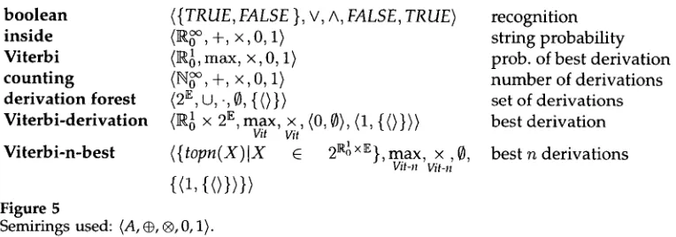
Figure 5

({TRUE, FALSE }, V, A, FALSE, TRUE)

+, x, o, 1>

(II~, max, x, O, 1) ( I ~ , +, ×,0, 1)

{0}>

(l~ 1 x 2E, max, x, (0,0>, (1, {(>}>>

Vii Vit

({topn(X)IX

E

2~ x~}, max, x , 0,

Vit-n

{0,{<>}>}>

Semirings used: {A, @, ®, 0,1/.

recognition string probability prob. of best derivation number of derivations set of derivations best derivation best n derivations

then the infinite sum is also less than or equal to that value. 3 This important property makes it easy to compute, or at least approximate, infinite sums.

There will be several especially useful semirings in this paper, which are defined in Figure 5. We will write P~ to indicate the set of real numbers from a to b inclusive, with similar notation for the natural numbers, N. We will write E to indicate the set of all derivations in some canonical form, and 2 n to indicate the set of all sets of derivations in canonical form. There are three derivation semirings: the derivation forest semiring, the Viterbi-derivation semiring, and the Viterbi-n-best semiring. The operators used in the derivation semirings (., max, x, max, and x ) will be described

Vit Vit Vit-n Vit-n later, in Section 2.5.

The inside semiring includes all nonnegative real numbers, to be closed under addition, and includes infinity to be closed under infinite sums, while the Viterbi semiring contains only numbers up to 1, since under max this still leads to closure.

The three derivation forest semirings can be used to find especially important val- ues: the derivation forest semiring computes all derivations of a sentence; the Viterbi- derivation semiring computes the most probable derivation; and the Viterbi-n-best semiring computes the n most probable derivations. A derivation is simply a list of rules from the grammar. From a derivation, a parse tree can be derived, so the derivation forest semiring is analogous to conventional parse forests. Unlike the other semirings, all three of these semirings are noncommutative. The additive operation of these semirings is essentially union or maximum, while the multiplicative oper- ation is essentially concatenation. These semirings are described in more detail in Section 2.5.

2.2 Item-based Description

A semiring parser requires an item-based description of the parsing algorithm, in the form given earlier. So far, we have skipped one important detail of semiring parsing. In a simple recognition system, as used in deduction systems, all that matters is whether an item can be deduced or not. Thus, in these simple systems, the order of processing items is relatively unimportant, as long as some simple constraints are met. On the other hand, for a semiring such as the inside semiring, there are important ordering constraints: we cannot compute the inside value of an item until the inside values of

[image:8.468.52.434.57.191.2]

all of its children h a v e b e e n c o m p u t e d .

Thus, w e n e e d to i m p o s e an o r d e r i n g on the items, in such a w a y that no item precedes a n y item on w h i c h it d e p e n d s . We will assign each item x to a " b u c k e t " B, writing

bucket(x) = B

a n d saying that item x is associated with B. We o r d e r the buckets in such a w a y that if item y d e p e n d s on item x, t h e n

bucket(x) <_ bucket(y).

For some pairs of items, it m a y be that b o t h d e p e n d , directly or indirectly, o n each other; w e associate these items w i t h special " l o o p i n g " buckets, w h o s e values m a y require infinite sums to compute. We will also call a b u c k e t looping if an item associated w i t h it d e p e n d s on itself.

One w a y to achieve a b u c k e t i n g with the required ordering constraints (suggested b y F e r n a n d o Pereira) is to create a g r a p h of the d e p e n d e n c i e s , with a n o d e for each item, a n d an edge from each item x to each item b that d e p e n d s on it. We then separate the g r a p h into its strongly connected c o m p o n e n t s (maximal sets of n o d e s all reachable from each other), a n d p e r f o r m a topological sort. Items f o r m i n g singleton strongly connected c o m p o n e n t s are associated w i t h their o w n buckets; items f o r m i n g n o n s i n g l e t o n strongly connected c o m p o n e n t s are associated w i t h the same looping bucket. See also Section 5.

Later, w h e n w e discuss algorithms for interpreting an item-based description, w e will n e e d a n o t h e r concept. Of all the items associated with a b u c k e t B, w e will be able to find derivations for only a subset. If w e can derive an item x associated w i t h b u c k e t B, w e write x E B, a n d say that item x is in bucket B. For example, the goal item of a parser will almost always be

associated

w i t h the last bucket; if the sentence is grammatical, the goal item will be

in

the last bucket, a n d if it is not grammatical, it will not be.

It will be useful to a s s u m e that there is a single, variable-free goal item, a n d that this goal item does not occur as a condition for a n y rules. We c o u l d always a d d a

[old-goal]

n e w goal item

~oal]

a n d a rule

~oal]

w h e r e

[old-goal] is the goal in the original

description.

2.3 The Grammar

A semiring parser also requires a g r a m m a r as input. We will n e e d a list of rules in the grammar, a n d a function,

R(rule),

that gives the v a l u e for each rule in the grammar. This latter function will be semiring-specific. For instance, for c o m p u t i n g the inside a n d Viterbi probabilities, the v a l u e of a g r a m m a r rule is just the conditional probability of that rule, or 0 if it is not in the grammar. For the Boolean semiring, the v a l u e is

TRUE

if the rule is in the grammar,

FALSE

otherwise.

R(rule)

replaces the set of rules R of a conventional g r a m m a r description; a rule is in the g r a m m a r if R(rule) ~ O.

2.4 Conditions for Correct Processing

We will say that a semiring parser w o r k s correctly if, for a n y grammar, input, a n d semiring, the v a l u e of the i n p u t according to the g r a m m a r equals the v a l u e of the i n p u t using the parser. In this subsection, w e will define the v a l u e of an i n p u t according to the grammar, define the v a l u e of an i n p u t using the parser, a n d give a sufficient condition for a semiring parser to w o r k correctly. F r o m this p o i n t onwards, unless w e specifically m e n t i o n otherwise, w e will a s s u m e that some fixed semiring, item-based description, a n d g r a m m a r h a v e b e e n given, w i t h o u t specifically m e n t i o n i n g w h i c h ones.

Computational Linguistics Volume 25, Number 4

be simply the p r o d u c t (in the semiring) of the values of the rules u s e d in E:

m

VG(E) : @ R(ei)

i:1

Then w e can define the v a l u e of a sentence that can be d e r i v e d using g r a m m a r deriva- tions E 1, E 2 .. . . . E k to be:

k

v~ = ( D v~(EJ)

j=1

w h e r e k is potentially infinite. In other words, the v a l u e of the sentence according to the g r a m m a r is the s u m of the values of all derivations. We will a s s u m e that in each g r a m m a r formalism there is some w a y to define derivations uniquely; for instance, in CFGs, one w a y w o u l d be using left-most derivations. For simplicity, w e will s i m p l y refer to derivations, rather than, for example, left-most derivations, since w e are n e v e r interested in n o n u n i q u e derivations.

A short example will help clarify. We consider the following grammar:

s ~

AA a(S-+AA)

A --+ A A a ( A - + A A )

A --+ a R ( A - + a )

(2)

a n d the i n p u t string aaa. There are t w o g r a m m a r derivations, the first of w h i c h

~ S - - + A A , , A - - + A A , , --A---+a . .A---+a --A---+a

is ~ => A m ~ A A A ~ a A A ~ aaA ~ aaa, w h i c h has v a l u e R ( S --+ A A ) ® R ( A --+ A A ) ® R ( A --+ a) ® R ( A --+ a) ® R ( A --+ a). Notice that the rules in the v a l u e are the same rules in the same o r d e r as in the derivation. The other g r a m m a r deriva-

~ S - - * A A - - ~ A - - * a ~ A - - + A A _ _ ~ A - - * a _ _ A - - * a

tion is ~ ~ .4.4 ~ aA => a A A ~ aaA => aaa, w h i c h has v a l u e R ( S --+ A A ) ® R ( A --+ a) ® R ( A -+ A A ) ® R ( A --+ a) ® R ( A ---* a). The v a l u e of the sentence is the s u m of the values of the t w o derivations,

[R(s --+ AA) ® R(A -+ AA) 0 a ( A --+ a) ® R(A --+ ~) ® R(A --+ a)] • [a(S --+ AA) O R(A --+ a) ® R(A --+ AA) ® R(A -* a) ® R(A --+ ~)]

2.4.2 I t e m D e r i v a t i o n s . Next, w e define item derivations, i.e., derivations using the item-based description of the parser. We define item d e r i v a t i o n in such a w a y that for a correct parser description, there is exactly one item d e r i v a t i o n for each g r a m m a r derivation. The v a l u e of a sentence using the parser is the s u m of the v a l u e of all item derivations of the goal item. Just as with g r a m m a r derivations, i n d i v i d u a l item derivations are finite, b u t there m a y be infinitely m a n y item or g r a m m a r derivations of a sentence.

sS--•AA----A-•AA---A-.-•a

- - - - A . - + a --A.--~a =:~ A A :=~ A A A ::~ a A A =~ a a A =:~ a a a

G r a m m a r Derivation

R(S --+ AA)

R(A ~

~

-

~

a)

a)

G r a m m a r Derivation Tree

[1, S, 4]

R( S

,4]

-

-

+

~

A

~

R ( A --~ a)

R(A

,3]

I

I

_

R(A--+a) _ R ( A ~ a )

I t e m Derivation ] t e e

R(S -~ AA) ® R(A ~ AA) ® R(A --+ a) ® R(A ~ a) ® R(A -+ a)

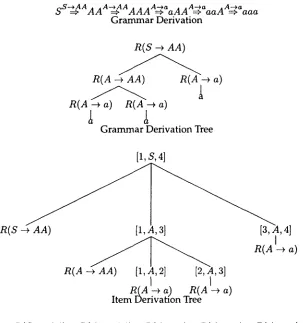
Derivation Value

Figure 6

Grammar derivation, grammar derivation tree, item derivation tree, and derivation value.

tree for x just gives a w a y of d e d u c i n g x f r o m the g r a m m a r rules. We define a n i t e m d e r i v a t i o n tree recursively. The b a s e case is rules of the g r a m m a r : (r / is a n i t e m d e r i v a t i o n tree, w h e r e r is a rule of the g r a m m a r . Also, if Dal . . .

Da k, Dcl

. . . Dcj are d e r i v a t i o n trees h e a d e d b y

al... ak, Cl... Cj

respectively, a n d if ~ c l . . . cj is the instantiation of a d e d u c t i o n rule, t h e n (b: D~ 1 .. . . . D~k/ is also a d e r i v a t i o n tree. Notice that the

De1 • •. Dq do n o t occur in this tree: t h e y are side conditions, a n d a l t h o u g h their

existence is r e q u i r e d to p r o v e that cl • .. cj could be d e r i v e d , t h e y d o n o t contribute to the v a l u e of the tree. We will w r i t e a l . . . ak b to indicate that there is an i t e m deri- v a t i o n tree of the f o r m (b:

Da,

. . .

Dakl.

As m e n t i o n e d in Section 2.2, w e will write

x E B if bucket(x) = B a n d there is an i t e m d e r i v a t i o n tree for x.

We can c o n t i n u e the e x a m p l e of p a r s i n g aaa, n o w u s i n g the i t e m - b a s e d CKY p a r s e r of Figure 3. There are t w o i t e m d e r i v a t i o n trees for the goal item; in Figure 6, w e give the first as an e x a m p l e , d i s p l a y i n g it as a tree, rather t h a n w i t h angle b r a c k e t notation, for simplicity.

[image:11.468.38.341.58.381.2]

Computational Linguistics Volume 25, Number 4

w e can h a v e a one-to-one c o r r e s p o n d e n c e b e t w e e n i t e m d e r i v a t i o n s a n d g r a m m a r derivations; loops in the g r a m m a r lead to an infinite n u m b e r of g r a m m a r derivations, a n d an infinite n u m b e r of c o r r e s p o n d i n g i t e m derivations.

A g r a m m a r including rules s u c h as

S --, AAA A --+ B A ~ a

B --* A B --,

w o u l d a l l o w d e r i v a t i o n s s u c h as S ~ A A A ~ B A A ~ A A ~ BA ~ A ~ B ~ e.

We w o u l d include the exact s a m e i t e m d e r i v a t i o n s h o w i n g A ~ B ~ ~ three times. Similarly, for a d e r i v a t i o n s u c h as A ~ B ~ A ~ B ~ A =~ a, w e w o u l d h a v e a c o r r e s p o n d i n g i t e m d e r i v a t i o n tree that i n c l u d e d m u l t i p l e uses of the A --* B a n d B --* A rules.

2.4.3 Value of I t e m D e r i v a t i o n . The v a l u e of a n i t e m d e r i v a t i o n D, V(D), is the p r o d u c t of the v a l u e of its rules, R(r), in the s a m e o r d e r that t h e y a p p e a r in the i t e m d e r i v a t i o n tree. Since rules occur o n l y in the leaves of i t e m d e r i v a t i o n trees, the o r d e r is precisely d e t e r m i n e d . For a n i t e m d e r i v a t i o n tree D w i t h rule v a l u e s dl, d2 . . . dj as its leaves,

J

V(D) = @ R(di)

i=1

(3)

Alternatively, w e can write this e q u a t i o n r e c u r s i v e l y as

[R(D)

if D is a rule

V(D) = I@~--1 V(Di) if D = (b: D 1 , . . . , Dk} (4)

C o n t i n u i n g o u r e x a m p l e , the v a l u e of the i t e m d e r i v a t i o n tree of Figure 6 is

R(s

AA) ® R(A

a) ® R(A

AA) ® R(A

a) ® R(A

a)

the s a m e as the v a l u e of the first g r a m m a r derivation.

Let inner(x) r e p r e s e n t the set of all i t e m d e r i v a t i o n trees h e a d e d b y an i t e m x. T h e n the v a l u e of x is the s u m of all the v a l u e s of all i t e m d e r i v a t i o n trees h e a d e d b y x. Formally,

V(x)=

V(D)

DEinner(x)

The v a l u e of a sentence is just the v a l u e of the goal item, V(goal).

item derivation will have the same value for any commutative semiring and any rule value function. In this case, we say that the derivations are commutatively iso-valued.

Finishing our example, the value of the goal item given our example sentence is just the sum of the values of the two item-based derivations,

[R(S ---* AA) @ R(A --~ AA) @ R(A --~ a) @ R(A ~ a) @ R(A ---*

a)] @

[R(S ~ A A ) ® R(A ~ a) ® R(A - . A A ) ® R(A ~ a) ® R(A ~

a) l

This value is the same as the value of the sentence according to the grammar.

2.4.5 Conditions for Correctness. We can now specify the conditions for an item-based description to be correct.

Theorem 1

Given an item-based description I, if for every grammar G, there exists a one-to-one correspondence between the item derivations using I and the grammar derivations, and the corresponding derivations are iso-valued, then for every complete semiring, the value of a given input wl ... wn is the same according to the grammar as the value of the goal item. (If the semiring is commutative, then the corresponding derivations need only be commutatively iso-valued.)

Proof

The proof is very simple; essentially, each term in each sum occurs in the other. By hypothesis, for a given input, there are grammar derivations E1 . . . Ek (for 0 < k < o0) and corresponding item derivation trees D1 .. • Dk of the goal item. Since corresponding items are iso-valued, for all i, V(Ei) ~- V(Di). (If the semiring is commutative, then since the items are commutatively iso-valued, it is still the case that for all i, V(Ei) --

V(Di).) Now, since the value of the string according to the grammar is just

(~i

V(Ei) =

(~i V(Di), and the value of the goal item is E)i V(Di), the value of the string according

to the grammar equals the value of the goal item. []

There is one additional condition for an item-based description to be usable in practice, which is that there be only a finite number of derivable items for a given input sentence; there may, however, be an infinite number of derivations of any item.

2.5 The Derivation Semirings

All of the semirings we use should be familiar, except for the derivation semirings, which we now describe. These semirings, unlike the other semirings described in Figure 5, are not commutative under their multiplicative operator, concatenation.

In m a n y parsers, it is conventional to compute parse forests: compact represen- tations of the set of trees consistent with the input. We will use a related concept, derivation forests, a compact representation of the set of derivations consistent with the input, which corresponds to the parse forest for CFGs, but is easily extended to other formalisms.

Often, we will not be interested in the set of all derivations, but only in the most probable derivation. The Viterbi-derivation semiring computes this value. Alterna- tively, we might want the n best derivations, which would be useful if the output of the parser were passed to another stage, such as semantic disambiguation; this value is computed by the Viterbi-n-best derivation semiring.

Computational Linguistics Volume 25, Number 4

rule value. Instead of g r a m m a r rule concatenation, w e p e r f o r m string concatena- tion. The d e r i v a t i o n semiring t h e n c o r r e s p o n d s to n o n d e t e r m i n i s t i c transductions; the Viterbi semiring c o r r e s p o n d s to a w e i g h t e d or probabilistic transducer; a n d the Viterbi-n-best semiring could be u s e d to get n-best lists from probabilistic transduc- ers.

2.5.1 D e r i v a t i o n Forest. The d e r i v a t i o n forest semiring consists of sets of derivations, w h e r e a d e r i v a t i o n is a list of rules of the grammar. 4 Sets containing one rule, such as

{ (X --* Y Z ) } for a CFG, constitute the primitive elements of the semiring. The additive o p e r a t o r kJ p r o d u c e s a u n i o n of derivations, a n d the multiplicative o p e r a t o r - p r o d u c e s the concatenation, one d e r i v a t i o n c o n c a t e n a t e d w i t h the next. The concatenation op- eration (.) is d e f i n e d o n b o t h derivations a n d sets of derivations; w h e n a p p l i e d to a set of derivations, it p r o d u c e s the set of pairwise concatenations. The additive identity is s i m p l y the e m p t y set, 0: u n i o n w i t h the e m p t y set is an identity operation. The multiplicative identity is the set containing the e m p t y derivation, {0}: c o n c a t e n a t i o n w i t h the e m p t y d e r i v a t i o n is an identity operation. Derivations n e e d not be complete. For instance, for CFGs, {(X --* YZ, Y ~ y)} is a valid element, as is {(Y --* y, X ~ x)}. In fact, {(X ~ A, B --* b)} is a valid element, a l t h o u g h it could not occur in a valid g r a m m a r derivation, or in a correctly functioning parser. A n e x a m p l e of concatenation of sets is {(A ~ a),(B ~ b)}. {(C ~ c),(D ~ d)} = {(A ~ a,C -+ c),(A --* a,D

a), (B

b, C

c), (B

b, D - . a)}.

Potentially, d e r i v a t i o n forests are sets of infinitely m a n y items. H o w e v e r , it is still possible to store t h e m using finite-sized representations. Elsewhere ( G o o d m a n 1998), w e s h o w h o w to i m p l e m e n t d e r i v a t i o n forests efficiently, using pointers, in a m a n n e r analogous to the typical i m p l e m e n t a t i o n of parse forests, a n d also similar to the w o r k of Billot a n d Lang (1989). Using these techniques, b o t h u n i o n a n d concatenation can be i m p l e m e n t e d in constant time, a n d e v e n infinite u n i o n s will be r e a s o n a b l y efficient.

2.5.2

Viterbi-derivation Semiring.

The Viterbi-derivation semiring c o m p u t e s the m o s t probable d e r i v a t i o n of the sentence, g i v e n a probabilistic grammar. Elements of this semiring are a pair, a real n u m b e r v a n d a d e r i v a t i o n forest E, i.e., the set of derivations w i t h score v. We define max, the additive operator, as

Vit

(v,E) if v > w

m a x ( ( v , E ) , ( w , D ) ) = (w,D) i f v < w

Vit ( V , E kJ D) if v = w

In typical practical Viterbi parsers, w h e n t w o derivations h a v e the same value, one of the derivations is arbitrarily chosen. In practice, this is usually a fine solution, a n d one that c o u l d be u s e d in a real-world i m p l e m e n t a t i o n of the ideas in this paper, b u t f r o m a theoretical v i e w p o i n t , the arbitrary choice destroys the associative p r o p e r t y of the additive operator, max. To preserve associativity, w e keep d e r i v a t i o n forests of all ele- m e n t s that tie for beret.

The definition for m a x is only d e f i n e d for t w o elements. Since the o p e r a t o r is Vit

associative, it is clear h o w to define m a x for a n y finite n u m b e r of elements, b u t w e also Vit

n e e d infinite s u m m a t i o n s to be defined. We use the s u p r e m u m , sup: the s u p r e m u m of a set is the smallest v a l u e at least as large as all elements of the set; that is, it is a

m a x i m u m that is defined in the infinite case. We can n o w define m a x for the case of

vit

infinite sums. Let

W ~- s u p V (v,E>6X

D = {EI<w,E> E X}

Then m a x X = (w, D/. D is potentially empty, b u t this causes us no p r o b l e m s in

vit

theory, a n d will not occur in practice. We define x as

vit

(v, E I vXit(w, D> = (v x w, E. D>

w h e r e E • D represents the concatenation of the t w o derivation forests.

2.5.3 Viterbi-n-best Semiring. The last kind of derivation semiring is the Viterbi-n- best semiring, w h i c h is used for constructing n-best lists. Intuitively, the v a l u e of a string using this semiring will be the n m o s t likely derivations of that string (unless there are f e w e r than n total derivations.) In practice, this is actually h o w a Viterbi-n-best semiring w o u l d typically be i m p l e m e n t e d . From a theoretical v i e w p o i n t , however, this i m p l e m e n t a t i o n is inadequate, since w e m u s t also define infinite stuns a n d be sure that the distributive p r o p e r t y holds. Elsewhere ( G o o d m a n 1998), w e give a m a t h e m a t i c a l l y precise definition of the semiring that handles these cases.

3. Efficient Computation of Item Values

Recall that the v a l u e of an item x is just V(x) = (~Deinner(x)V(D), the s u m of the values of all derivation trees h e a d e d b y x. This definition m a y require s u m m i n g o v e r exponentially m a n y or e v e n infinitely m a n y terms. In this section, w e give relatively efficient formulas for c o m p u t i n g the values of items. There are three cases that m u s t be handled. First is the base case, w h e n x is a rule. In this case, inner(x) is trivially {(x/}, the set containing the single d e r i v a t i o n tree x. Thus, V(x) = (~Dcinner(x) V(D) = (~DC{<x)} V(D) = V((x>) = R(x)

The second and third cases occur w h e n x is an item. Recall that each item is asso- ciated w i t h a bucket, and that the buckets are ordered. Each item x is either associated with a n o n l o o p i n g bucket, in w h i c h case its v a l u e d e p e n d s only on the values of items in earlier buckets; or with a l o o p i n g bucket, in w h i c h case its value d e p e n d s poten- tially on the values of other items in the same bucket. In the case w h e n the item is associated with a n o n l o o p i n g bucket, if we c o m p u t e items in the same o r d e r as their buckets, we can a s s u m e that the values of items al . . . ak contributing to the value of item b are k n o w n . We give a f o r m u l a for c o m p u t i n g the v a l u e of item b that d e p e n d s only on the values of items in earlier buckets.

Computational Linguistics Volume 25, Number 4

3.1 Item Value Formula Theorem 2

If an item x is not in a looping bucket, then

k

V(x) ----

(~

(~ V(ai)

i:1

al... ak s.t. al.x. al~

(5)

Proof

Let us expand our notion of inner to include deduction rules:

i n n e r ( ~ )

is the set

of all derivation trees of the form (b: ( a l . . . / ( a 2 . . . / - . .

(ak...11"

For any item derivation

tree that is not a simple rule, there is some al...ak, b such that D E

i n n e r ( ~ ) .

Thus, for any item x,

v(x) =

( ~

v(D)

DE inner( x )

=

(~

(~

V(D)

(6)

al...al¢ s.t. al'~c, ak DEinner(aI"x" ak)

Consider item derivation trees

Dal ... Dak

headed by items al . . .

ak

such that ~ g ~ .

Recall that (x:

Da, .... , Dakl

is the item derivation tree formed by combining each of

these trees into a full tree, and notice that U (x:

Dal,..., Dakl = i n n e r ( ~ ) .

Da I ff inner( al ) ... Da k ff inner (ak )

( 9

v(o) =

( 9

D6inner(al "~c" ak) Da I 6 i n n e r ( a J ... Da k 6inner(ak)

Therefore

=

G

Da 16inner(al ) ... Da k ff inner( ak )

k

i = 1 Dai Cinner(ai)

k : ( 9 V(,,i)

i=1

Substituting this back into Equation 6, w e get

k

V(K)= ( ~

( ~ V ( a , )

i = 1 al... ak s.t. al.x. ai

v(Ix: Da, . . . . ,Dak))

k

(~V(Dai)

i=1

Now, w e address the case in w h i c h x is an item in a l o o p i n g bucket. This case requires c o m p u t a t i o n of an infinite sum. We will write out this infinite sum, a n d discuss h o w to c o m p u t e it exactly in all cases, except for one, w h e r e w e a p p r o x i m a t e it.

Consider the derivable items

x l . . . Xm in

some looping b u c k e t B. If w e build u p d e r i v a t i o n trees incrementally, w h e n w e begin processing b u c k e t B, o n l y those trees with n o items f r o m b u c k e t B will be available, w h a t w e will call z e r o t h generation derivation trees. We can p u t these z e r o t h generation trees together to f o r m first gener- ation trees, h e a d e d b y elements in B. We can combine these first generation trees w i t h each other a n d w i t h z e r o t h g e n e r a t i o n trees to f o r m second generation trees, a n d so on. Formally, we define the generation of a d e r i v a t i o n tree h e a d e d b y x in bucket B to be the largest n u m b e r of items in B w e can e n c o u n t e r on a p a t h from the root to a leaf.

Consider the set of all trees of g e n e r a t i o n at most g h e a d e d b y x. Call this set

inner<_~(x, B). We can define the K g

generation value of an item x in b u c k e t B, V<_~(x, B):

V<_g(x,B) =

( ~

V(D)

D 6 inner<g (x,B)

Intuitively, as g increases, for

x E B, inner<~(x, B)

b e c o m e s closer a n d closer to

inner(x).

That is, the finite s u m of values in the f o r m e r a p p r o a c h e s the infinite s u m of values in the latter. For w-continuous semirings (which includes all of the semirings considered in this paper), an infinite s u m is equal to the s u p r e m u m of the partial sums (Kuich 1997, 613). Thus,

V(x) =

( ~

V(D)

= sup

V<g(x, B)

OC inner( x,B ) g

It will be easier to c o m p u t e the s u p r e m u m if w e find a simple f o r m u l a for

V<_g(x, B).

Notice that for items x E B, there will be n o generation 0 derivations, so V_<0(x, B) = 0. Thus, generation 0 m a k e s a trivial base for a recursive formula. Now, w e can consider the general case:

Theorem 3

For x an item in a looping b u c k e t B, and for g ~ 1,

V<g(x,B)

i=1 [ V<_g-l(ai, B ) al... ak s.t. al'x" ak

if ai ~ B

if ai E B (7)

The p r o o f parallels that of T h e o r e m 2 ( G o o d m a n 1998).

3.2 Solving the Infinite Summation

A f o r m u l a for

V<_g(x, B)

is useful, b u t w h a t w e really n e e d is specific techniques for c o m p u t i n g the s u p r e m u m ,

V(x)

= supg V<<_g(x, B). For all w-continuous semirings, the s u p r e m u m of iteratively a p p r o x i m a t i n g the v a l u e of a set of p o l y n o m i a l equations, as w e are essentially d o i n g in Equation 7, is equal to the smallest solution to the equations (Kuich 1997, 622). In particular, consider the equations:

k ~V(ai)

if ai ~ B

V<_oo(x,B) =

0

~ [ V<_oo(ai,

B)

if

a

i

C B

(8)

i:1

Computational Linguistics Volume 25, Number 4

where

V<~(x, B)

can be thought of as indicating [B[ different variables, one for each item x in the looping bucket B. Equation 7 represents the iterative approximation of Equation 8, and therefore the smallest solution to Equation 8 represents the supremum of Equation 7.

One fact will be useful for several semirings: whenever the values of all items x E B at generation g + 1 are the same as the values of all items in the preceding generation, g, they will be the same at all succeeding generations, as well. Thus, the value at generation g will be the value of the supremum. Elsewhere (Goodman 1998), we give a trivial proof of this fact.

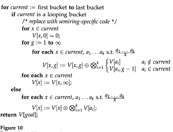
Now, we can consider various semiring-specific algorithms for computing the supremum. Most of these algorithms are well known, and we have simply extended them from specific parsers (described in Section 7) to the general case, or from one semiring to another.

Notice in this section the wide variety of different algorithms, one for each semi- ring, and some of them fairly complicated. In a conventional system, these algorithms are interweaved with the parsing algorithm, conflating computation of infinite sums with parsing. The result is algorithms that are both harder to understand, and less portable to other semirings.

We first examine the simplest case, the Boolean semiring. Notice that whenever a particular item has value

TRUE

at generation g, it must also have value

TRUE

at generation g + 1, since if the item can be derived in at most g generations then it can certainly be derived in at most g + 1 generations. Thus, since the number of

TRUE

valued items is nondecreasing, and is at most IB[, eventually the values of all items must not change from one generation to the next. Therefore, for the Boolean semiring, a simple algorithm suffices: keep computing successive genera- tions, until no change is detected in some generation; the result is the supremum. We can perform this computation efficiently if we keep track of items that change value in generation g and only examine items that depend on them in generation g + l . This algorithm is then similar to the algorithm of Shieber, Schabes, and Pereira (1993).

For the counting semiring, the Viterbi semiring, and the derivation forest semi- ring, we need the concept of a derivation subgraph. In Section 2.2 we considered the strongly connected components of the dependency graph, consisting of items that for some sentence could possibly depend on each other, and we put these possibly interdependent items together in looping buckets. For a given sentence and gram- mar, not all items will have derivations. We will find the subgraph of the dependency graph of items with derivations, and compute the strongly connected components of this subgraph. The strongly connected components of this subgraph correspond to loops that actually occur given the sentence and the grammar, as opposed to loops that might occur for some sentence and grammar, given the parser alone. We call this subgraph the derivation subgraph, and we will say that items in a strongly connected component of the derivation subgraph are part of a loop.

nite n u m b e r of derivations, a n d thus an infinite value. C o m p u t e items that d e p e n d directly or indirectly on items in loops: these items also have infinite value. A n y other items can o n l y be d e r i v e d in finitely m a n y w a y s using items in the current bucket, so c o m p u t e successive generations until the values of these items do not change.

The m e t h o d for solving the infinite s u m m a t i o n for the derivation forest semiring d e p e n d s on the i m p l e m e n t a t i o n of derivation forests. Essentially, that representation will use pointers to efficiently represent derivation forests. Pointers, in various forms, allow one to efficiently represent infinite circular references, either directly ( G o o d m a n 1999), or indirectly ( G o o d m a n 1998). Roughly, the algorithm we will use is to c o m p u t e the derivation subgraph, a n d then create pointers analogous to the directed edges in the d e r i v a t i o n subgraph, including pointers in loops w h e n e v e r there is a loop in the derivation s u b g r a p h (corresponding to an infinite n u m b e r of derivations). Details are given elsewhere ( G o o d m a n 1998). As in the finite case, this representation is equivalent to that of Billot a n d Lang (1989).

For the Viterbi semiring, the algorithm is analogous to the Boolean case. Deriva- tions using loops in these semirings will always have values no greater than deriva- tions not using loops, since the value with the loop will be the same as some v a l u e w i t h o u t the loop, multiplied b y some set of rule probabilities that are at most 1. Since the additive operation is max, these l o w e r (or at m o s t equal) looping derivations do not change the v a l u e of an item. Therefore, w e can s i m p l y c o m p u t e successive generations until values fail to change f r o m one iteration to the next.

Now, consider i m p l e m e n t a t i o n s of the Viterbi-derivation semiring in practice, in w h i c h w e keep only a representative derivation, rather than the w h o l e deriva- tion forest. In this case, loops d o not change values, and w e use the same algo- r i t h m as for the Viterbi semiring. In an i m p l e m e n t a t i o n of the Viterbi-n-best semi- ring, in practice, loops can change values, b u t at m o s t n times, so the same algo- r i t h m used for the Viterbi semiring still works. Elsewhere ( G o o d m a n 1998), we de- scribe theoretically correct i m p l e m e n t a t i o n s for b o t h the Viterbi-derivation a n d Viterbi- n-best semirings that keep all values in the e v e n t of ties, p r e s e r v i n g addition's associativity.

The last semiring w e consider is the inside semiring. This semiring is the most difficult. There are two cases of interest, one of w h i c h w e can solve exactly, a n d the other of w h i c h requires approximations. In m a n y cases involving looping buckets, all

a l x

d e d u c t i o n rules will be of the f o r m ~ - , w h e r e al a n d b are items in the l o o p i n g bucket, a n d x is either a rule, or an item in a p r e v i o u s l y c o m p u t e d bucket. This case corre- s p o n d s to the items u s e d for d e d u c i n g singleton productions, such as those Earley's algorithm uses for rules of the f o r m A --* B a n d B --+ A. In this case, Equation 8 forms a set of linear equations that can be solved b y matrix inversion. In the m o r e general case, as is likely to h a p p e n with epsilon rules, w e get a set of nonlinear equations, a n d m u s t solve t h e m b y a p p r o x i m a t i o n techniques, such as simply c o m p u t i n g successive generations for m a n y iterations. 5 Stolcke (1993) p r o v i d e s an excellent discussion of these cases, including a discussion of sparse matrix inversion, useful for speeding u p some computations.

Computational Linguistics Volume 25, Number 4

goal

Derivation of [goal]

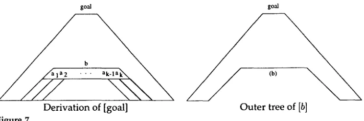
Figure 7

Outside algorithm.

goal

Outer tree of [b]

4. R e v e r s e V a l u e s

The previous section showed how to compute several of the most commonly used values for parsers, including Boolean, inside, Viterbi, counting, and derivation forest values, among others. Noticeably absent from the list are the outside probabilities, which we define below. In general, computing outside probabilities is significantly more complicated than computing inside probabilities.

In this section, we show h o w to compute outside probabilities from the same item-based descriptions used for computing inside values. Outside probabilities have many uses, including for reestimating grammar probabilities (Baker 1979), for im- proving parser performance on some criteria (Goodman 1996b), for speeding parsing in some formalisms, such as data-oriented parsing (Goodman 1996a), and for good thresholding algorithms (Goodman 1997).

We will show that by substituting other semirings, we can get values analogous to the outside probabilities for any commutative semiring; elsewhere (Goodman 1998) we have shown that we can get similar values for many noncommutative semirings as well. We will refer to these analogous quantities as reverse values. For instance, the quantity analogous to the outside value for the Viterbi semiring will be called the reverse Viterbi value. Notice that the inside semiring values of a hidden Markov model (HMM) correspond to the forward values of HMMs, and the reverse inside values of an H M M correspond to the backwards values.

Compare the outside algorithm (Baker 1979; Lari and Young 1990), given in Fig- ure 7, to the inside algorithm of Figure 2. Notice that while the inside and recognition algorithms are very similar, the outside algorithm is quite a bit different. In particular, while the inside and recognition algorithms looped over items from shortest to longest, the outside algorithm loops over items in the reverse order, from longest to shortest. Also, compare the inside algorithm's main loop formula to the outside algorithm's main loop formula. While there is clearly a relationship between the two equations, the exact pattern of the relationship is not obvious. Notice that the outside formula is about twice as complicated as the inside formula. This doubled complexity is typical of outside formulas, and partially explains w h y the item-based description format is so useful: descriptions for the simpler inside values can be developed with relative ease, and then automatically used to compute the twice-as-complicated outside values. 6

[image:20.468.58.430.55.179.2]

goal

[image:21.468.33.404.54.173.2]

Derivation of [goal]

Figure 8

goal

O u t e r tree of [b]

Item derivation tree of [goal] and outer tree of [b].

For a context-free grammar, using the CKY parser of Figure 3, recall that the inside probability for an item [i, A, j] is

P(A -~ wi... wj-1).

The outside probability for the same item is

P(S G

w l . . . W i _ l A W j . , . Wn). T h u s , the outside probability has the p r o p e r t y that w h e n multiplied b y the inside probability, it gives the probability that the start symbol generates the sentence using the given item,

P(S G Wl

. . , w i _ d A w j . . . Wn G Wl . . . Wn).

This probability equals the s u m of the probabilities of all derivations using the given item. Formally, letting

P(D)

represent the probability of a particular derivation, a n d

C(D, [i, X,j])

represent the n u m b e r of occurrences of item [i,

X,j] in

d e r i v a t i o n D (which

for some parsers could be m o r e than one if X w e r e part of a loop),

inside(i, X,j) x outside(i, X,j) =

Z

P(D) C(D, [i, X,j])

D a derivation

The reverse values in general h a v e an analogous meaning. Let

C(D, x)

represent the n u m b e r of occurrences (the count) of item x in item derivation tree D. Then, for a n item x, the reverse v a l u e

Z(x)

s h o u l d h a v e the p r o p e r t y

V(x) ®

Z(x) =

V(D)C(D, x)

(9)

D a derivation

Notice that w e h a v e multiplied an e l e m e n t of the semiring, V(D), b y an integer,

C(D, x).

This multiplication is m e a n t to indicate r e p e a t e d addition, using the additive operator of the semiring. Thus, for instance, in the Viterbi semiring, m u l t i p l y i n g b y a c o u n t other t h a n 0 has no effect, since x ® x = max(x, x) = x, while in the inside semiring, it c o r r e s p o n d s to actual multiplication. This v a l u e represents the s u m of the values of all d e r i v a t i o n trees that the item x occurs in; if an item x occurs m o r e than once in a derivation tree D, then the v a l u e of D is c o u n t e d m o r e than once.

To formally define the reverse v a l u e of an item x, w e m u s t first define the o u t e r trees

outer(x).

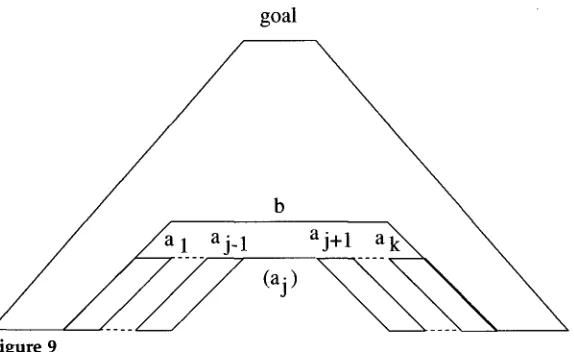
C o n s i d e r an item d e r i v a t i o n tree of the goal item, containing one or m o r e instances of item x. R e m o v e one of these instances of x, a n d its children too, leaving a gap in its place. This tree is an outer tree of x. Figure 8 shows an item d e r i v a t i o n tree of the goal item, including a subderivation of an item b, d e r i v e d from terms al . . . . ,

ak.

It also shows an outer tree of b, with b a n d its children r e m o v e d ; the spot b was r e m o v e d f r o m is labeled (b).

Computational Linguistics Volume 25, Number 4

For an outer tree D E

outer(x),

w e define its value, Z(D), to be the p r o d u c t of the values of all rules in D,

(~rCD R(r).

Then, the reverse v a l u e of an item can be formally defined as

Z(x)= 0

Z(D)

(10)

DEouter( x )

That is, the reverse v a l u e of x is the s u m of the values of each o u t e r tree of x. Now, w e s h o w that this definition of reverse values has the p r o p e r t y described b y Equation 9. 7

Theorem 4

V(x) ®

z(x) =

E)

v(D)C(D, x)

D a d e r i v a t i o n

Proof

First, observe that

V(x) ®Z(x)= ( E]~ V(I)) ® 0 Z(O)= (~

~ V(I)®Z(O)

(11)

\lEinner(x) Ocouter(x) IEinner(x) OEouter(x)

Next, w e argue that this last expression equals the expression on the r i g h t - h a n d side of Equation 9, (~D

V(D)C(D,x).

For an item x, a n y o u t e r part of an item d e r i v a t i o n tree for x can be c o m b i n e d w i t h a n y inner part to f o r m a c o m p l e t e item d e r i v a t i o n tree. That is, a n y O E

outer(x)

a n d a n y I E

inner(x)

can be c o m b i n e d to f o r m an item derivation tree D containing x, a n d a n y item d e r i v a t i o n tree D containing x can be d e c o m p o s e d into such o u t e r a n d inner trees. Thus, the list of all combinations of o u t e r a n d inner trees c o r r e s p o n d s exactly to the list of all item d e r i v a t i o n trees containing x. In fact, for an item d e r i v a t i o n tree D containing

C(D, x)

instances of x, there are

C(D, x)

w a y s to f o r m D f r o m combinations of o u t e r a n d inner trees. Also, notice that for D c o m b i n e d from O a n d I

V(I) ® Z(O) = ( ~ R ( r ) ® ( ~ R ( r ) = ( ~ R ( r ) = V(D)

rEI rEO rED

T h u s ,

{~

(~ V(I) ® Z(O)

= ( ~

V(D)C(D,x)

IEinner(x) OEouter(x) D C o m b i n i n g Equation 11 w i t h Equation 12, w e see that

(12)

V(x) o

z(x) =

0

V(D)C(O, x)

D a derivation

c o m p l e t i n g the proof. []