Sparse Kernel Canonical Correlation Analysis
Delin Chu, Li-Zhi Liao, Michael K. Ng and Xiaowei Zhang
Abstract—Canonical correlation analysis (CCA) is a multi-variate statistical technique for finding the linear relationship between two sets of variables. The kernel generalization of CCA named kernel CCA has been proposed to find nonlinear relations between data sets. Despite the wide usage of CCA and kernel CCA, they have one common limitation that is the lack of sparsity in their solution. In this paper, we consider sparse kernel CCA and propose a novel sparse kernel CCA algorithm (SKCCA). Our algorithm is based on a relationship between kernel CCA and least squares. Sparsity of the dual transformations is introduced by penalizing the`1-norm of dual vectors. Experiments demonstrate that our algorithm not only performs well in computing sparse dual transformations but also can alleviate the over-fitting problem of kernel CCA.
Index Terms—canonical correlation analysis, kernel, sparsity
I. INTRODUCTION
T
HE description of relationship between two sets of variables has long been an interesting topic to many researchers. Canonical correlation analysis (CCA) [10] is a multivariate statistical technique for finding the linear relationship between two sets of variables. It seeks a linear transformation for each of the two sets of variables in a way that the projected variables in the transformed space are maximally correlated. In recent years, CCA has been successfully applied in various areas, including genomic data analysis [19], [20] and bilingual analysis [18], where researchers can measure multiple sets of variables on a single subject. For instance, DNA copy number variations, gene expression, and single nucleotide polymorphism (SNP) data might all be available on a common set of patient samples.Since CCA only consider linear transformation of the original variables, it fails to capture nonlinear relations. How-ever, in a wide range of practical problems linear relations may not be adequate for studying relation among variables. Detecting nonlinear relations among data is important and useful in modern data analysis, especially when dealing with data that are not in the form of vectors, such as text documents, images, microarray data and so on. A natural extension, therefore, is to explore and exploit nonlinear rela-tions among data. Among nonlinear extensions of CCA, one most frequently used approach is the kernel generalization
Manuscript received 11 Oct. 2012; accepted 8 Nov. 2012.
Delin Chu and Xiaowei Zhang are with Department of Mathematics, Na-tional University of Singapore, Block S17, 10 Lower Kent Ridge Road Sin-gapore 119076. Email: [email protected]/[email protected]. These two authors are supported in part by NUS Research Grant R-146-000-140-112.
Li-Zhi Liao is with Department of Mathematics, Hong Kong Baptist University, Kowloon Tong, Hong Kong. Email: [email protected]. This author is supported in part by GRF grants HKBU201409 and HKBU201611 from the Research Grant Council of Hong Kong.
Michael K. Ng is with Centre for Mathematical Imaging and Vision, and Department of Mathematics, Hong Kong Baptist University, Kowloon Tong, Hong Kong. E-mail: [email protected]. This author is supported in part by grants from Hong Kong Baptist University (FRG), and the Research Grant Council of Hong Kong.
of CCA, named kernel canonical correlation analysis (kernel CCA) [1], [3]. Kernel CCA have been successfully applied in many fields, including content−based image retrieval [9], bioinformatics [21] and independent component analysis [3]. Despite the wide usage of CCA and kernel CCA, they have one common limitation that is the lack of sparsity in their solution. For CCA, the lack of sparsity makes the interpretation of extracted features difficult, while for kernel CCA it can lead to excessive computational time to compute projections of new data since kernel functions must be evaluated at all training data. To handle the limitation of CCA, researchers suggested to incorporate sparsity into weight vectors and many attempts have been made to study sparse CCA [6], [8], [19], [20]. Similarly, we shall find sparse solutions for kernel CCA so that projections of new data can be computed by evaluating the kernel function at a subset of the training data. Another motivation for studying sparse kernel CCA is the over-fitting problem of kernel CCA as pointed out in [3], [9]. Although there are many sparse kernel approaches [5], seldom can be found in the area of sparse kernel CCA [4], [16].
In this paper we consider a new sparse kernel CCA approach. A relationship between CCA and least squares is established so that CCA solutions can be obtained by solving a least squares problem. Since the optimization criteria of CCA and kernel CCA are of the same form, this relationship can be extended to kernel CCA. Based on the relationship, we attempt to introduce sparsity to kernel CCA by penalizing
`1-norm of the solutions, which eventually leads to a ` 1-norm regularized least squares problem having the form of the following basis pursuit denoising (BPDN) problem
min x∈Rd
1
2kAx−bk
2
2+λkxk1, (1.1)
whereλ >0is a regularizer controlling the sparsity ofx. We adopt a fixed-point continuation (FPC) method [7] to solve the BPDN problem above, which results in a new sparse kernel CCA algorithm named SKCCA.
The remainder of the paper is organized as follows. In Section II, we present background results of both CCA and kernel CCA. In Section III, we establish a relationship between CCA and least squares problems. In Section IV, we extend the relationship to kernel CCA and incorporate sparsity into kernel CCA by penalizing the least squares with
`1-penalty. Solving the penalized least squares problems by FPC leads to a new sparse kernel CCA algorithm. Numerical results of applying the newly proposed algorithm to content-based image retrieval are presented in Section V. Finally, we draw some conclusions in Section VI.
II. BACKGROUND
Let{xi}ni=1∈Rd1 and{yi}ni=1∈Rd2 bensamples for variablesx∈Rd1 andy∈Rd2, respectively. Denote
and assume both {xi}ni=1 and{yi}ni=1 have zero mean, i.e.,
n
P
i=1
xi = 0and n
P
i=1
yi = 0. Then CCA solves the following
optimization problem
max wx,wy
wTxXYTwy
s.t. wTxXXTwx= 1, wTyY YTwy= 1,
(2.1)
to get the first pair ofweight vectorswxandwy, which are
further utilized to obtain the first pair ofcanonical variates wTxX and wyTY, respectively. However, only one pair of weight vectors is not enough for most practical problems. To obtain multiple projections of CCA, we recursively solve the above optimization problem with additional constraint that the current canonical variates must be orthogonal to all previous ones. Specifically, denotingWx= [wx1 · · · wxl]and Wy = [wy1 · · · wly], we use the trace formula
max Wx,Wy
Trace(WT
xXYTWy)
s.t. WxTXXTWx=I, Wx∈Rd1×l, WyTY YTWy=I, Wy∈Rd2×l.
(2.2)
as the criterion of CCA to compute multiple projections. In kernel methods, we first implicitly represent data as elements in reproducing kernel Hilbert spaces associated with positive definite kernels, then apply linear algorithms on the data and substitute the linear inner product by kernel functions, which results in nonlinear variants. The main idea of kernel CCA is that we first virtually map data X into a high dimensional feature space Hx via a mappingφx such
that data in the feature space become
Φx=φx(x1) · · · φx(xn)∈RNx×n,
whereNx is the dimension of feature spaceHxthat can be
very high or even infinite. The mappingφxfrom input data to
the feature spaceHxis performed implicitly by considering
apositive definite kernel function κx satisfying
κx(x1, x2) =hφx(x1), φx(x2)i, (2.3)
whereh·,·iis an inner product inHx, rather than by giving
the coordinates of φx(x)explicitly. The feature spaceHx is
known as theReproducing Kernel Hilbert Space (RKHS)[2] associated with kernel functionκx. In the same way, we can
map Y into a feature space Hy associated with kernel κy
through mappingφy such that
Φy=φy(y1) · · · φy(yn)∈RNy×n.
After mappingXtoΦxandY toΦy, we then apply ordinary
linear CCA to data pair (Φx,Φy).
Let
Kx=hΦx,Φxi= [κx(xi, xj)]ni,j=1∈R
n×n, (2.4)
Ky=hΦy,Φyi= [κy(yi, yj)]ni,j=1∈R
n×n (2.5)
be matrices consisting of inner products of data setsΦxand Φy, respectively. Kx andKy are called kernel matricesor Gram matrices. Then kernel CCA seeks linear transformation in the RKHS by expressing the weight vectors as linear combinations of the training data, that is
wx= Φxα= n
X
i=1
αiφx(xi), wy= Φyβ= n
X
i=1
βiφy(yi),
where α, β ∈ Rn are called dual vectors. The first pair of dual vectors can be determined by solving the following optimization problem
max
α,β α
TK xKyβ
s.t. αTK2
xα= 1, βTK2
yβ= 1.
(2.6)
To compute multiple pairs of dual vectors, we consider
max
Wx,Wy
Trace(WT
xKxKyWy)
s.t. WxTKx2Wx=I, Wx∈Rn×l,
WT
yKy2Wy =I, Wy∈Rn×l,
(2.7)
whereWx= [α1 · · · αl]andWy= [β1 · · · βl] consist of
dual vectors forX andY, respectively.
In the process of deriving (2.7), we assumed dataΦx and Φy have been centered (that is, the column mean of both Φx and Φy are zero) as X and Y, otherwise, we need to
perform data centering before applying kernel CCA. Unlike data centering ofXandY, we can not perform data centering directly on Φx andΦy since we do not know their explicit
coordinates. However, as shown in [12], [13], data centering inRKHScan be accomplished via some operations on kernel matrices. To centerΦx, a natural idea should be computing Φx,c= Φx(I−ene
T n
n ), whereendenotes column vector inRn
with all entries being 1. However, since kernel CCA makes use of the dataX through kernel matrix Kx, the centering
process can be performed onKx as
Kx,c=hΦx,c,Φx,ci= (I− eneTn
n )hΦx,Φxi(I− eneTn
n )
= (I−ene T n
n )Kx(I− eneTn
n ). (2.8)
Similarly, we can center testing dataΦx,t as
Kx,t,c=hΦx,c,Φx,t−Φx eneTN
n i
= (I−ene T n
n )Kx,t−(I− eneTn
n )Kx eneTN
n , (2.9)
whereN is the number of testing data and Kx,t denotes the
kernel matrix between training and testing data. More details about data centering inRKHScan be found in [12], [13]. In the sequel of this paper, we assume the kernel matrices have been centered.
III. CCAAND LEAST SQUARES
It is well known that CCA is closely related to linear regression problem, and some relation between CCA and linear regression has been established under the condition that rank(X) = n−1 and rank(Y) = d2 in [14], [15]. In this section, we establish a relation between CCA and linear regression without any additional constraint on X and Y. Before that, we consider the characterization of solutions of (2.2).
Definer=rank(X),s=rank(Y),m=rank(XYT)and t = min{r, s}. Let the (reduced) SVD factorizations of X
andY be, respectively,
X =U
Σ1
0
QT1 =
U1 U2
Σ1
0
QT1 =U1Σ1QT1,
and
Y =V
Σ2
0
QT2 =
V1 V2
Σ2
0
QT2 =V1Σ2QT2, (3.2)
where U ∈ Rd1×d1, U
1 ∈ Rd1×r, U2 ∈ Rd1×(d1−r),
Σ1 ∈ Rr×r, Q1 ∈ Rn×r, V ∈ Rd2×d2, V1 ∈ Rd2×s,
V2 ∈ Rd2×(d2−s), Σ2 ∈ Rs×s, Q2 ∈ Rn×s, U and V are orthogonal, Σ1 and Σ2 are nonsingular and diagonal,
Q1 andQ2 are column orthogonal. It follows from the two orthogonality constraints in (2.2) that
l≤min{rank(X),rank(Y)}=min{r, s}=t. (3.3)
Next, let
QT1Q2=P1ΣP2T (3.4)
be the singular value decomposition of QT
1Q2, whereP1∈
Rr×r andP2 ∈Rs×s are orthogonal and Σ∈Rr×s, then
m=rank(QT
1Q2)≤min{r, s}=t.
A solution subset of optimization problem (2.2) is de-scribed in the following lemma
Lemma 1: Any(Wx, Wy)of the following forms
Wx=U1Σ−11P1(:,1 :l) +U2E,
Wy =V1Σ−21P2(:,1 :l) +V2F,
(3.5)
where P1(:,1 : l) denotes the first l columns of P1, E ∈
R(d1−r)×l andF ∈R(d2−s)×l are arbitrary, is a solution of optimization problem (2.2).
The proof of Lemma 1 can be found in [6], where a full characterization of all solutions of optimization problem (2.2) has been established.
Based on the explicit expression of solutions of opti-mization problem (2.2), we can now establish a relationship between CCA and least squares. Let
Tx=YT[(Y YT)
1
2]†V1P2(:,1 :l)Σ(1 :l,1 :l)−1
=Q2P2(:,1 :l)Σ(1 :l,1 :l)−1, (3.6)
Ty=XT[(XXT)
1
2]†U1P1(:,1 :l)Σ(1 :l,1 :l)−1
=Q1P1(:,1 :l)Σ(1 :l,1 :l)−1, (3.7)
where A† denotes the Moore-Penrose inverse of a general matrix A and 1 ≤ l ≤ m, then we have the following theorem.
Theorem 2: For any l satisfying 1 ≤ l ≤ m, suppose
Wx∈Rd1×l andWy∈Rd2×l satisfy
Wx=argmin{kXTWx−Txk2F :Wx∈Rd1×l}, (3.8)
and
Wy=argmin{kYTWx−Tyk2F :Wy∈Rd2×l}, (3.9)
whereTxandTy are defined in (3.6) and (3.7), respectively.
Then Wx andWy form a solution of optimization problem
(2.2).
Proof: Since (3.8) and (3.9) have the same form, we only prove the result for Wx, the same idea can be applied
toWy.
We know that Wx is a solution of (3.8) if and only if it
satisfies the normal equation
XXTWx=XTx. (3.10)
Substituting factorizations (3.1), (3.2) and (3.4) into the equation above, we get
XXT =U1Σ21U
T
1 ,
and
XTx = U1Σ1QT1Q2P2(:,1 :l)Σ(1 :l,1 :l)−1
= U1Σ1P1(:,1 :l),
which yield an equivalent reformulation of (3.10)
U1Σ21U1TWx=U1Σ1P1(:,1 :l). (3.11)
It is easy to check thatWxis a solution of (3.11) if and only
if
Wx=U1Σ−11P1(:,1 :l) +U2E, (3.12)
whereE ∈R(d1−r)×l is an arbitrary matrix. Therefore, Wx
is a solution of (3.8) if and only ifWxcan be formulated as
(3.12).
Similarly,Wy is a solution of (3.9) if and only ifWy can
be written as
Wy =V1Σ−21P2(:,1 :l) +V2F, (3.13)
whereF ∈R(d2−s)×lis an arbitrary matrix.
Now, comparing equations (3.12) and (3.13) with the equation (3.5) in Lemma 1, we can conclude that for any solution Wx of the least squares problem (3.8) and any
solution Wy of the least squares problem (3.9), Wx and Wy form a solution of optimization problem (2.2), hence
a solution of CCA.
Remark 3.1: In Theorem 2 we only considerl satisfying
1 ≤l ≤m. This is reasonable, since there are m nonzero canonical correlations betweenX andY, and weight vectors corresponding to zero canonical correlation do not contribute to the canonical correlation between dataX andY.
IV. SPARSE KERNELCCA
Since kernel CCA criterion (2.7) and CCA criterion (2.2) have the same form, we can expect a similar characterization of solutions of (2.7) as Lemma 1. Define
ˆ
r=rank(Kx), sˆ=rank(Ky), mˆ =rank(KxKy),
and let the eigenvalue decomposition of Kx and Ky be,
respectively,
Kx=U
Π1 0
0 0
UT =
U1 U2
Π1 0
0 0
U1 U2
T
=U1Π1U1T, (4.1)
and
Ky =V
Π2 0
0 0
VT =
V1 V2
Π2 0
0 0
V1 V2
T
=V1Π2V1T, (4.2)
where
U ∈Rn×n, U1∈Rn׈r, U2∈Rn×(n−ˆr), Π1∈Rrˆ×rˆ, V ∈Rn×n, V1∈Rn×sˆ, V2∈Rn×(n−ˆs), Π2∈Rˆs×sˆ, U and V are orthogonal, Π1 and Π2 are nonsingular and diagonal. In addition, let
UT
be the singular value decomposition of U1TV1, where P1 ∈
Rrˆ×rˆ and
P2 ∈ Rˆs׈s are orthogonal and Π ∈ Rrˆ×sˆ is a diagonal matrix. Then we can prove for 1≤l ≤min{ˆr,sˆ}
that
Wx=U1Π−11P1(:,1 :l) +U2E, Wy=V1Π−21P2(:,1 :l) +V2F,
(4.4)
with E ∈ R(n−rˆ)×l and
F ∈ R(n−sˆ)×l being arbitrary
matrices, form a subset of solutions to (2.7).
Solutions of (2.7) can also be associated with least squares problems. Define
Tx=U1P1(:,1 :l), Ty=V1P2(:,1 :l), (4.5) with1≤l≤mˆ, then each pair of WxandWy, satisfying
Wx=argmin{kKxWx− Txk2F :Wx∈Rn×l},
and
Wy=argmin{kKyWy− Tyk2F :Wy∈Rn×l},
respectively, forms a solution of (2.7).
Motivated by research on lasso [17] which shows that sparsity can be obtained by penalizing`1-norm of the vari-ables, we incorporate sparsity into Wx andWy by solving
the following `1-norm regularized least squares problems
min 1
2kKxWx− Txk 2
F + l
P
i=1
λx,ikWx,ik1
subject to Wx∈Rn×l,
(4.6)
and
min 1
2kKyWy− Tyk 2
F+ l
P
i=1
λy,ikWy,ik1
subject to Wy∈Rn×l,
(4.7)
whereλx,i, λy,i>0are regularization parameters,Wx,iand
Wy,i are ith column ofWx andWy, respectively.
Since optimization problems (4.6) and (4.7) have the same form, all results holding for one problem can be naturally extended to the other, so we concentrate on (4.6). Note that when l = 1optimization problem (4.6) reduces to a BPDN problem of the form (1.1), which has been intensively studied in the field of compressed sensing. Many efficient approaches have been proposed to solve the BPDN problem, among which we adopt the fixed-point continuation (FPC) method [7], due to its simple implementation and nice convergence property.
Fixed-point algorithm for (1.1) is an iterative method which updates iterates as
xk+1=Sν xk−τ AT(Ax−b), withν =τ λ, (4.8)
where τ > 0 denotes the step size, and Sν is the
soft-thresholding operator defined as
Sν(x) =sign(x)max{|x| −ν,0}, x∈Rd, (4.9)
with denoting component-wise multiplication. Sν(x)
re-duces all components of x with magnitude less than ν to zero, thus reducing the`1-norm and introducing sparsity.
The fixed-point algorithm can be extended to solve (4.6), which yields
Wk+1
x,i =Sνx,i W
k
x,i−τxKxT(KxWx,ik − Tx,i), (4.10)
wherei= 1,· · · , l,νx,i=τxλx,i withτx>0 denoting the
step size.
Algorithm 1 Sparse kernel CCA (SKCCA)
Input: Training dataX ∈Rd1×n,Y ∈Rd2×n
1: Construct and center kernel matricesKx,Ky; 2: Compute matrix factorizations (4.1)-(4.3);
3: ComputeTx andTy defined in (4.5); 4: νx,i=τxλx,i,νy,i=τyλy,i,i= 1,· · ·, l, 5: repeat
6: Wx,ik+1=Sνx,i W
k
x,i−τxKx(KxTWx,ik − Tx,i), 7: untilconvergence
8: repeat
9: Wy,ik+1=Sνy,i W
k
y,i−τyKy(KyTWy,ik − Ty,i), 10: untilconvergence
Output: Sparse dual transformation matricesWxk andWyk.
We can prove that fixed-point iterations have some nice convergence properties which are presented in the following theorem. Proof of the theorem can be found in [7].
Theorem 3: Let Ωbe the solution set of (4.6), then there existsM∗∈Rn×lsuch that
KxT(KxWx− Tx)≡M∗, ∀ Wx∈Ω. (4.11)
In addition, define
L:={(i, j) :|Mi,j∗ |< λx,j} (4.12)
as a subset of indices and letλmax(KxTKx)be the maximum
eigenvalue ofKxTKx, and chooseτx from
0< τx< 2 λmax(KxTKx)
,
then the sequence {Wxk}, generated by the fixed-point iter-ations (4.10) starting with any initial point Wx0, converges
to someWx∗ ∈Ω. Moreover, there exists an integer K >0
such that
(Wk
x)i,j = (Wx∗)i,j= 0, ∀(i, j)∈L, (4.13)
whenk > K.
Remark 4.1: 1) Equation (4.11) shows that for any two optimal solutions of (4.6) the gradient of the squared Frobe-nius norm in (4.6) must be equal.
2) Equation (4.13) means that the entries of Wxk with indices from L will converge to zero in finite steps. The positive integer K is a function of W0
x and Wx∗, and
determined by the distance between them.
Similarly, we can design a fixed-point algorithm to solve (4.7) as follows:
Wk+1
y,i =Sνy,i W
k
y,i−τyKyT(KyWy,ik − Ty,i), (4.14)
wherei= 1,· · ·, l,νy,i=τyλy,i with τy >0 denoting the
step size.
Applying fixed-point iterations (4.10) and (4.14) to ` 1-norm regularized least squares problems (4.6) and (4.7), we get a new sparse kernel CCA algorithm presented in Algorithm 1.
Since canonical correlations in kernel CCA depend only on kernel matrices Kx and Ky. Therefore, as we shall
Proposition 4: Let rˆ= rank(Kx) andsˆ= rank(Ky). If ˆ
r+ ˆs= n+γ for some γ >0, then U1TV1 has at least γ singular values equal to 1.
Proof: Since U1 ∈ Rn×rˆ, U2 ∈ Rn×(n−ˆr) and V1 ∈
Rn׈s are column orthogonal and U1U1T +U2U2T =In, we have
(UT
1V1)TU1TV1=V1TU1U1TV1=Isˆ− V1TU2U2TV1. If there existγ >0such that rˆ+ ˆs=n+γ, thenn−ˆr= ˆ
s−γ <sˆand
rank(V1TU2U2TV1) =rank(U2TV1)≤n−r,ˆ
which impliesV1TU2U2TV1has at leastsˆ−(n−ˆr) =γzero eigenvalues. Thus,(UT
1V1)TU1TV1has at leastγeigenvalues equal to 1, which further implies that U1TV1 has at least γ singular values equal to 1.
In kernel methods, due to nonlinearity of kernel functions, the rank of kernel matrices is very close to n, which makes most canonical correlations to be 1. For instance, for Gaussian kernel
κ(x, y) =exp
−2σ12kx−yk 2
, σ6= 0 (4.15)
we can prove that the kernel matrix Kxgiven by (Kx)ij =
exp −2σ12kxi−xjk2
has full rank, provided that the points {xi}ni=1are distinct [12]. Thus, in kernel methods we usually have
ˆ
r=rank(Kx) =n−1, sˆ=rank(Ky) =n−1,
after centering data. In this case, all nonzero canonical correlations determined by the singular values of U1TV1 are equal to 1. This means ordinary kernel CCA fails to provide a useful estimation of canonical correlations for general kernels, because for any distinct sample{xi}ni=1 of variable
x and distinct sample {yi}ni=1 of variable y the canonical correlations returned by kernel CCA will be 1 even though variablesxandy have no joint information.
To avoid forementioned data over-fitting problem in kernel CCA, researchers suggested to design a regularized kernel-ization of CCA [3], [9]. On the other hand, as shown in [17], the `1-penalty term can alleviate data overfitting problem while at the same time introduce sparsity. We can expect that sparse kernel CCA (4.6)-(4.7) enjoys the properties of both computing sparse Wx, Wy and avoiding data over-fitting
similar to regularized kernel CCA.
V. EXPERIMENTS
In this section, we apply our newly proposed sparse kernel CCA algorithm SKCCA to content-based image retrieval (CBIR) by combining image and text data. CBIR is a challenging aspect of multimedia analysis and has become popular in past few years. Generally, it is the problem of searching for digital images in large databases by their visual content (e.g., color, texture, shape) rather than the metadata such as keywords, labels, and descriptions associated with the images. There exists study utilizing kernel CCA for image retrieval [9].
In the implementation of SKCCA, we need to determine regularization parameters {λx,i} and {λy,i}. We know that x∗ is a solution of BPDN problem (1.1) if and only if
0∈AT(Ax∗−b) +λ∂kx∗k1,
where ∂kx∗k1 is the subgradient of `1-norm k · k1 at x∗. It follows that x = 0 is the solution of (1.1) when λ ≥
kATbk∞. To avoid zero solution, which is meaningless in practice, we chose
λx,i=γxkKxTTx,ik∞, λy,i=γykKyTTy,ik∞, i= 1,· · ·, l,
where0< γx, γy<1.
AMATLABcode implementing FPC algorithm for BPDN problem, named FPC BB [22], is publicly available. We used this code in our implementation of Algorithm 1 with xtol=10−5 and mxitr=104 and all other parameters de-fault.
We experiment on the Ground Truth Image Database [23] created at the University of Washington, which consists of 21 data sets of outdoor scene images. In our experiment we used 852 images form 19 data sets that have been annotated with keywords. We exploited text features and low-level image features, including color and texture, and applied sparse kernel CCA to perform image retrieval from text query. We used the bag-of-words approach to represent the text associated with images, Gabor filters to extract texture features and HSV (hue-saturation-value) color representation as color features.
Following previous work [9], we used Gaussian kernel
kx(Ii, Ij) =exp
−kIi−Ijk 2
2σ2
,
whereIi is a vector concatenating texture features and color
features ofith image andσis the minimum distance between different images, to compute kernel matrix Kx for the first
view. The linear kernel was employed to compute kernel matrix Ky using text features for the other view. We used
217 images as training data and the rest were used as testing data.
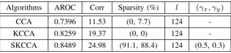
We compare the performance of CCA, kernel CCA and SKCCA in TABLE I, where the accuracy of image retrieval is measured by average area under the ROC curve (AROC), and for a collection of queries we use the average of retrieval precision of all queries as the average retrieval precision of this collection. More details about the evaluation of retrieval performance can be found in [6]. Results in TABLE I were obtained by lettingl= ˆm=rank(KxKy), that is, projections
corresponding to all nonzero canonical correlations were used. ‘Corr’ denotes the summation of canonical correlations between testing data, ‘Sparsity’ column records sparsity of both Wx and Wy, which is the percentage of zero entries
in the matrices. The first component records sparsity ofWx
while the second component records sparsity of Wy. The
‘(γx, γy)’ column records value of regularization parameters
[image:5.595.310.543.695.749.2]in SKCCA.
TABLE I: CCA, kernel CCA and SKCCA for content-based image retrieval.
Algorithms AROC Corr Sparsity (%) l (γx, γy)
CCA 0.7396 11.53 (0, 7.7) 124 -KCCA 0.8259 19.37 (0, 0) 124 -SKCCA 0.8489 24.98 (91.1, 88.4) 124 (0.5, 0.3)
0 20 40 60 80 100 120 0.55
0.6 0.65 0.7 0.75 0.8 0.85
Number of columns of (Wx,Wy) used
Average AROC
[image:6.595.56.285.52.228.2]CCA KCCA SKCCA
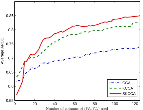
Fig. 1: Content-based image retrieval using CCA, kernel CCA and SKCCA with 217 images in the training data and 635 images in testing data.
larger summation of canonical correlations between testing data than other two approaches, which empirically shows that SKCCA is better than CCA for finding nonlinear relations and alleviates the over-fitting problem of KCCA. We can also see that sparsity of the dual projections Wx and Wy
computed by SKCCA is greater than88%, which can exces-sively reduce the computational time of computing projection of a new data in practice as we only need to evaluate kernel functions between the new data and a small subset of training data.
In Fig. 1, we plot AROC of CCA, kernel CCA and SKCCA as a function of the number of projections used (i.e., differentl). As visible in Fig. 1, the AROC of all approaches gradually increases when more projections are used for re-trieval. This is reasonable, beacause when we increaselmore projections corresponding to nonzero canonical correlations are used for retrieval and these added projections may convey information contained in the training data. In addition, we observe that the AROC of SKCCA is at first smaller than and then exceeds that of kernel CCA. This indicates that when suitable number of dual projections are used for retrieval SKCCA can improve the performance of kernel CCA.
VI. CONCLUSIONS
In this paper we proposed a novel sparse kernel CCA algorithm called SKCCA. This algorithm is based on a relationship between kernel CCA and least squares which is an extension of a similar relationship between CCA and least squares. We incorporated sparsity into kernel CCA by penalizing the `1-norm of dual vectors. The resulting ` 1-regularized minimization problems were solved by a fixed-point continuation (FPC) algorithm. Empirical results show that SKCCA not only performs well in computing sparse dual transformations, but also alleviates the over-fitting problem of kernel CCA.
Several interesting questions and extensions remain. In many applications such as genomic data analysis, CCA is often performed on more than two data sets. It will be helpful to extend sparse kernel CCA to deal with multiple data sets. In the derivation of SKCCA, we did not discuss the choice of kernel function. However, it is believed that the performance
of kernel CCA depends on the choice of the kernel. As for future research, we plan to study the problem of finding the optimal kernel of kernel CCA for different applications, as in the case of kernel FDA [11]. Moreover, we also plan to generalize the idea of sparse kernel CCA in this paper to involve multiple kernels.
REFERENCES
[1] S. Akaho, “A Kernel Method For Canonical Correlation Analysis”,In Proceedings of the International Meeting of the Psychometric Society, 2001.
[2] N. Aronszajn, “Theory of Reproducing Kernels,”Transactions of the American Mathematical Society, vol. 68, no. 3, pp. 337-404, 1950. [3] F. Bach and M. Jordan, “Kernel Independent Component Analysis”,
Journal of Machine Learning Research, vol. 3, pp. 1-48, 2003. [4] S. Balakrishnan, K. Puniyani and J. Lafferty, “Sparse Additive
Func-tional and Kernel CCA,”Proceedings of 29th International Conference of Machine Learning, 2012.
[5] C. M. Bishop,Pattern Recognition and Machine Learning, Springer, 2006.
[6] D. Chu, L. Liao, M. K. Ng and X. Zhang, “Sparse Canonical Correlation Analysis: New Formulation and Algorithm,”Submitted. [7] E. T. Hale, W. Yin and Y. Zhang, “Fixed-Point Continuation for`1
-Minimization: Methodology and Covergence,”SIAM J. Opt., vol. 19, no. 3, pp. 1107-1130, 2008.
[8] D. R. Hardoon and J. R. Shawe-Tayler, “Sparse Canonical Correlation Analysis,”Machine Learning, vol. 83, no. 3, pp. 331-353, 2011. [9] D. R. Hardoon, S. R. Szedmak and J. R. Shawe-Taylor, “Canonical
Correlation Analysis: an Overview with Application to Learning Methods,”Neural Computation, vol. 16, no. 12, pp. 2639-2664, 2004. [10] H. Hotelling, “Relations between Two Sets of Variables,”Biometrika,
vol. 28, pp. 321-377, 1936.
[11] S. Kim, A. Magnani and S. Boyd, “Optimal Kernel Selection in Kernel Fisher Discriminant Analysis,”The 23th Int’l Conf. Machine Learning, 2006.
[12] B. Sch¨olkopf and A. Smola,Learning with Kernels : Support Vector Machines, Regularization, Optimization, and Beyond, MIT Press, 2002.
[13] B. Sch¨olkopf, A. Smola and K. M¨uller, “Nonlinear Component Anal-ysis as a Kernel Eigenvalue Problem,”Neural Computation, vol. 10, pp. 1299-1319, 1998.
[14] L. Sun, S. Ji and J. Ye, “A Least Squares Formulation for Canonical Correlation Analysis,” InThe 25th Int’l Conf. Machine Learning, pp. 1024-1031, 2008.
[15] L. Sun, S. Ji and J. Ye, “Canonical Correlation Analysis for Multi-Label Classification: A Least Squares Formulation, Extensions and Analysis,”IEEE Trans. Pattern Anal. Mach. Intell., vol. 33, no. 1, pp. 194-200, 2011.
[16] L. Tan and C. Fyfe, “Sparse Kernel Canonical Correlation Analysis”,
Proceedings of 9th European Symposium on Artificial Neural Net-works,pp. 335-340, 2001.
[17] R. Tibshirani, “Regression Shrinkage and Selection via the Lasso,”
Journal of the Royal Statistical Society (Series B), vol. 58, pp. 267-288, 1996.
[18] A. Vinokourov, J. R. Shawe-Taylor and N. Cristianini, “Inferring a Semantic Representation of Text via Cross-Language Correlation Analysis,” In S.Becker, S.Thrun and K. Obermayer (eds.),Advances in Neural Information Processing Systems, Cambridge:MIT Press, 2003. [19] D. M. Witten and R. Tibshirani, “Extensions of Sparse Canonical Correlation Analysis with Applications to Genomic Data,”Statistical Applications in Genetics and Molecular Biology, 8, 2009. Issue 1, Article 28.
[20] D. M. Witten, R. Tibshirani and T. Hastie, “A Penalized Matrix Decomposition, with Applications to Sparse Principal Components and Canonical Correlation Analysis,”Biostatistics, vol. 10, no. 3, pp. 515-534, 2009.
[21] Y. Yamanishi, J. P. Vert, A. Nakaya and M. Kanehisa, “Extraction of Correlated Gene Clusters from Multiple Genomic Data by Generalized Kernel Canonical Correlation Analysis,”Bioinformatics, vol. 19(Suppl 1), pp. i323–i330, 2003.
[22] MATLAB Code for FPC BB, http://www.caam.rice.edu/
∼optimization/L1/fpc/.