©IJRASET: All Rights are Reserved
1744
Study of routing protocols for wireless sensor
networks
Vatsal Gupta
Electronics and Communication Engineering, MAIT, GGSIP University, Delhi
Abstract: Wireless sensor networks consist of plenty of nodes, which sense, compute and transmit certain physical quantities. These quantities are then transmitted to a recording station for obtaining inferences from the readings taken by those sensor nodes. For WSNs to work, connection & communication between nodes become important and thus, different routing techniques were proposed. The two main hurdles in designing a routing technique are - power management of the nodes and transmission speed of the nodes. Keeping in mind these two major problems, numerous routing protocols were given which depend upon the application and network topology. Out of the various routing protocols, LEACH (Low-Energy Adaptive Clustering Hierarchy) is one which belongs to hierarchal based routing techniques. Simulation of LEACH [1] protocol and its comparison with simple direct transmission method has been done on MATLAB-R2017a. From the results and the graphs obtained, it can be clearly understood that former is much better than the latter. In terms of network lifetime, first node death, transmission speed, data aggregation and on many other parameters, LEACH protocol, as in [1], outperforms basic direct routing protocol.
Keywords:Wireless Sensor Networks, LEACH Protocol, Flooding, SPIN, PEGASIS, Directed Diffusion, GEAR
I. INTRODUCTION
Wireless sensor networks (WSNs) are spatially distributed networks, intended for monitoring and recording certain quantities to be studied at a centralized location for an administrator to judge results. The quantities mentioned here include pollution levels, sound, temperature, humidity, heat signatures, speed, and many others. The environment where these can be employed are physical world, a biological system, or an information technology (IT) framework.
Sensors are electronic devices which observe changes in environment and transmit the information collected to a system, particularly a computer. Sensors used in any WSN or in any other system are either rechargeable battery operated or solar energy powered. In the era, where technology is advancing progressively and more work is being assigned to the machines & decreasing human labour; WSNs provide a way for seamless and reliable process for determining and examining physical environmental phenomenon. These networks are primarily used for military applications, smart homes, automobile parts monitoring, telemonitoring of human physiological data, etc.
Connectivity amongst the nodes is an important issue, of which several ideas have been put forth by experts to make the network energy-efficient and more productive. A WSN system includes: radio transmission antenna, microcontrollers, an electronic circuit, power source etc., which operates through some unguided medium (electromagnetic waves like Wi-Fi, 3G or 4G, etc.).
In this paper, study of routing protocols for WSNs are studied. Furthermore, LEACH (Low-Energy Adaptive Clustering Hierarchy) [1] protocol is simulated on a software and then compared with another protocol. This another protocol is basic direct routing protocol which is also simulated and their results are compared over a number of executions. The approach in LEACH protocol is based on cluster formation. Cluster is a special group of nodes, not necessarily involving all the nodes, which collect data and transmit it to a cluster head. Cluster head is assigned the work of sensing as well as collecting the other cluster member nodes data and transmit the collected information to a base station. Each node can become a cluster head and so, the process of selecting a node as cluster head needs special algorithms based on various factors like distance from base station, residual power, nearest node, etc. We began with a single cluster in a specified area but the same approach can be extended for a larger area.
II. LITERATURESURVEY
A. Routing techniques for WSN
©IJRASET: All Rights are Reserved
1745
work here as the number of nodes used are generally above hundred and that too randomly placed. Innovative techniques which eliminate energy inefficiencies are thus highly required.
Hence, comprehensive studies and research on these issues have been done and many researchers have put forth a number of routing techniques/methodologies. Routing protocols can be primarily classified according to their network structure, i.e. hierarchical, flat or location-based. Further classification of these protocols can be specified as query-based, multipath-based, negotiation-based, coherent-based, and QoS-based; depending on the protocol procedure [2].
1) Flooding: This is one of the initial protocols for data transfer as well as dissemination in any network. K. Sohraby, D. Minoli and T. Znati in [2] had briefly described it. For path sighting and information dissemination, this technique is often used in both wired and wireless ad-hoc networks. It does not require costly network topology maintenance because of its simple routing strategy. In flooding, each node senses a quantity and transmits it in the form of data packet to all the connected nodes. Upon receiving, the nodes send collected packets to their neighboring connected nodes. This process continues until that packet finds a discontinuity in the network, till it reaches its destination. This reception and transmission process of nodes has been depicted in Fig. 1. Further, as soon as the network topology changes, the data packets find new routes to travel. Flooding causes replication of data packets by network nodes indefinitely; till the data packet reaches its destination.
Fig. 1 Flooding protocol in data communication networks [2]
To prevent a packet from circulating indefinitely in the network, a hop count field is usually included in the packet. The hop count is almost set to the diameter of the network, initially; but as the packet travels across the network, it is decremented by one for each hop that it traverses. The process halts when the hop count equals zero and in that case, the packet is simply discarded. Obviously, after that, the packet is no longer forwarded. Flooding can be additionally enhanced by perceiving the data, thereby forcefully dropping all the packets that have already been forwarded from each network node. This strategy exclusively requires a system to continuously monitor the traffic and maintain a recent traffic history, to keep a track of the packets which have already been forwarded.
A variant of flooding known as selective flooding exists, in which, the data packet is sent to the routers which are present in the same direction. The routers do not send the incoming packet to every node it is attached to, but only to those which approximately lie on the same line.
As mentioned above, the process is quite simple and requires low maintenance cost. Still, it suffers from the following drawbacks.
2) Susceptibility to traffic implosion. This effect is observed when duplicate data packets are sent to the same node repeatedly.
a) The overlapping problem. This is caused when a node receives a data packet containing similar information from two or more different neighboring nodes.
b) This is the most severe one. It is called resource blinding. It comes into play when the energy constraints of the sensor nodes aren’t considered. As such, the node’s energy may get depleted rapidly, reducing the lifetime of the network.
A new, similar protocol known as gossiping was proposed which solved the implosion problem and other shortcomings of flooding. Gossiping ensures that the data packet explores a new path. In this protocol, rather than sending the incoming data packet to all the neighbours, each node randomly selects a neighbour and transmits the incoming data packet to it. Then that randomly selected node further sends the data packet to one of its neighbours which has also been randomly selected. This process iterates itself until the intended destination node receives the data packet or the maximum hop count exceeds.
©IJRASET: All Rights are Reserved
1746
connected sensor node in the network. SPIN majorly eliminates the deficiencies of conventional information propagation techniques to overcome their performance inefficiencies. SPIN majorly believes in data negotiation and resource adaptation. Here, data-negotiation needs that nodes participating in SPIN, before any transmission, knows about the contents of the data. This is done for negotiations before transmitting actual data, by first sending meta-data from the sender node to all the receiving nodes. A receiver node which shows interest in that advertised data by examining that meta-data sends a request for that data content. This form of negotiation implies that data is sent to only interested nodes, hence reducing the cause of data redundancy and eliminating traffic implosion & data overlap. In Fig. 2, all the three processes which nodes practice are shown. Another process known as resource adaption is there which allows sensor nodes to modify their tasks according to the present state of energy resources available. Each node has its own linked resource manager which keeps track of its resource consumption before any transmission or processing task. When the current energy of a node becomes low, it cuts down its associated tasks like forwarding meta-data and data packets, either to some extent or fully. This quality extends the lifetime of a network.
Fig.2 SPIN data negotiation process [2]
For negotiation process and data transmission, nodes running SPIN, practice three types of messages.
First, ADV, is used to advertise data with nodes. The network node advertises its data by first transmitting an ADV message containing the metadata with the remaining nodes of the network.
Second, REQ is used to request the advertised data of interest. After receiving an ADV containing metadata, a network node interested in receiving that specific data sends an REQ message to the metadata advertising node.
[image:3.595.203.419.442.595.2]Third, DATA holds the actual data collected by a sensor, along with a metadata header. The data message is typically larger as compared to the ADV and REQ messages. The latter messages only cover the metadata that are significantly smaller than the corresponding data message. The whole process, depicting SPIN is explained using a small model below in Fig. 3.
Fig. 3 Basic SPIN protocol operations [2]
Here, A is the data source sensor node, B is A’s immediate neighbour sensor node and all the other sensor nodes i.e. c, d, e, f, g are B’s immediate neighbour sensor nodes.
©IJRASET: All Rights are Reserved
1747
In [3], it’s been concluded that naming of data through meta-data descriptors and their use in negotiations solved the problem of traffic implosion and overlapping problem as discussed in flooding protocol. Furthermore, SPIN can majorly benefit a mobile sensors environment as their forwarding decisions are dependent upon local neighbourhood information. When comparing 1 and SPIN-2, Heinzelman et. al. concluded that SPIN-1 is better than classic flooding as it consumes at much 25% of energy as a classic flooding protocol. Moreover, SPIN-2 could disseminate 60% more data per unit energy than flooding.
4) Low-Energy Adaptive Clustering Hierarchy (LEACH): W. R. Heinzelman, A. Chandrakasan, and H. Balakrishnan in the year 2000, presented a cluster-based routing protocol named LEACH [1] which aimed at distributing the total energy of the network among the sensor nodes by the means of transposition of local cluster base stations, based on a randomized algorithm. It is a routing algorithm, intended for delivering the data collected from sensors grouped in some specific fashion to a data sink, namely a Base Station. The main objectives of LEACH are:
a) Extension of the network run-time
b) Reduced energy consumption by each sensor node
c) Use of data collection to lessen the quantity of communication messages
LEACH is self-organizing, hence, adaptive clustering. It employs randomization for distributing the energy load among the sensor nodes in the network.
The assumptions made in the LEACH protocol are:
1. All nodes can transmit with enough power to reach the base station.
2. Every node has sufficient computational powers to sustain different MAC (Medium access control) protocols.
3. Nodes positioned nearby to each other have correlated or similar data.
LEACH implements a MAC based hierarchical style methodology to set the network into a set of clusters. Each cluster is supervised by a selected cluster head (which can change over time). Since a cluster head can change over time, each sensor node in the network must be capable enough to become a cluster head. This appointment of a node as a cluster head has an advantage of evenly distributing the energy load among the sensor nodes in the network.
The cluster head has some duties. Its first task is to collect data from the cluster members, periodically. After gathering the data from its members, it is aggregated by the cluster head & redundancy is removed among associated values. Its second task is to transmit the aggregated data right to the base station in a single hop (one of the conditions of LEACH protocol). Its third task is to generate a TDMA (Time-Division Multiple Access) based schedule whereby each node of the cluster is given a time slot that it can use for transmission. Fig. 4 is a basic diagram showing how nodes transmit data to their respective cluster heads and then, how the cluster heads communicate with the base station/data sink.
For reducing any chances of collisions among sensors in the neighbourhood of the cluster, nodes implementing LEACH use CDMA (code division multiple access) grounded system of communication.
Fig.4 LEACH network model [2] LEACH protocol consists of two phases: [4]
1) Set-up phase
2) Steady phase
©IJRASET: All Rights are Reserved
1748
T(n) =
– ∗ ( ∗ ( , ) ) , ꓯ n ϵ G
T(n) = 0, ꓯ n ϵ G Where, T(n) is the threshold.
P is the cluster head probability. Its equal to (L is the number of nodes and gets decreased by 1 in each round). R is equal to current round.
G is the set of nodes that have not been selected to become cluster heads in the last 1/P rounds.
Node becomes cluster head if the value of T (n) is greater than a random number generated by a node, say, t; where t varies from 0 to 1. If the value of t (belonging to a particular node) satisfies the above criterion, that node becomes a cluster head. Once a node becomes a cluster head, then it cannot become a cluster head again until all the other nodes of that cluster have become cluster head once. This is required for balanced power consumption which in turn increases the run-time of the network.
Newly appointed cluster head then advertises about itself becoming the cluster head to the rest of the network. Thereafter, the other nodes send a join request to the cluster head, conveying their interest in becoming a part of the cluster. This is done by taking into consideration the received signal strength among other factors. After this transmission, they turn off their transmitters and turn them on, once they want to communicate with the cluster head. This helps in conserving their energy. Upon cluster creation, the cluster head makes and distributes TDMA schedule for the cluster member nodes. A CDMA code is selected by each cluster head and distributed to its cluster member nodes. In the steady phase, the member nodes then transmit their collected data to the cluster head in a single hop according to their allotted time. This data collection is done periodically.
Simulation results, like that of this paper, have shown that it is a better routing algorithm amongst its predecessors. LEACH protocol enhances a networks run-time in many ways: [1] [4]
a) As it is a self-adjusting algorithm, the periodic change in the appointment of a cluster head ensures that a node does not die out quickly by conserving its energy.
b) Since individual nodes are not required to send data to the base station themselves, data aggregation technique used by clusters contributes to greater energy saving. This also ensures the reduction of data traffic.
c) It does not require any control guidelines from the base station as well as no prerequisite facts of the network.
d) No prerequisite facts of the network configuration and control information from the base station is required.
e) Simulation results as shown in [1] revealed that the first death of a node under LEACH protocol occurred over 8 times later than in direct transmission protocol.
Despite these benefits, LEACH suffers numerous limitations: [4]
a) LEACH does not give any idea about the number of cluster heads in the network.
b) Due to any reason if the cluster head expires then that whole cluster will become unserviceable as the data assembled by the cluster member nodes would not be able to reach the base station.
c) Clusters are divided arbitrarily, which results in irregular distribution of sensor nodes. Like, some cluster may have lesser number of nodes and some other may have a greater number of nodes. Some cluster heads are placed at the center of the cluster and some cluster heads may be placed at the edge of the cluster. This phenomenon can cause rise in energy consumption and have great influence on the performance of the entire network.
d) Although the probability is low, considering a case where a node is not a part of any cluster, it will have to perform all the tasks on his own, which might take a toll on its energy resource.
In [1], it has been concluded that the energy distribution amongst the nodes has been highly effective in reducing energy dissipation which results in the enhancement of network lifetime. It further concluded that LEACH protocol reduces the communication energy approximately by 8 times as compared by basic direct routing protocol. Furthermore, the first death and the last death of the sensor nodes in LEACH protocol occurred over 8 times and 3 times later respectively, than the basic direct routing protocol.
5) Power-Efficient Gathering in Sensor Information Systems (PEGASIS): S. Lindsey & C. S. Raghavendra in 2001 [5] proposed PEGASIS which they claimed to be better than LEACH. PEGASIS comes under routing and information gathering protocols. It has the basic two following objectives:
a) To make a network highly energy-efficient and achieve uniform energy distribution amongst the nodes.
©IJRASET: All Rights are Reserved
1749
a) There is a homogeneous set of nodes installed across a geographical area.
b) Nodes have global knowledge related to other sensors’ locations.
c) To cover arbitrary ranges, nodes have the capacity to adjust their power.
PEGASIS is a nearly optimal, chain-based protocol. The elementary idea of PEGASIS is that, the nodes are required to only communicate with their nearest neighbors and the network nodes take turns to communicate with the base station. When this round of chain communication is ended, a new round is started.
Nodes here are equipped with CDMA based radio transceivers. The construction of chain starts from the farthest sensor node with respect to the base station. From the farthest node from the sink, network nodes are added progressively in the chain and this process ends when end node has been approached. Nodes which lie outside the current chain are added in the chain in a greedy fashion. The nearest node from the top node of the chain is added first, until all the nodes are included. To determine the closest neighbour, the node uses its signal strength to measure the distance. Then by using this information, it alters its signal strength according to its nearest neighbours position.
After this, a sensor node within the PEGASIS implementing chain is elected as a leader and data from either end is forwarded towards the leader node. This is done for every round wherein the round is managed by the base station. Here, the leaders’ role is to send the aggregated information to the base station. The chain leader is changed after every round. This ensures that amongst all the network nodes, energy is uniformly distributed. In case the chain leader is located far from the base station, then it will have to use very high power in order to transmit the data to the base station.
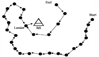
[image:6.595.229.398.426.524.2]Data aggregation in chain can be performed sequentially. Firstly, the chain leader issues a token to the farthest node in a direction, say, right direction for instance. The farthest node upon collecting the token then sends its aggregated data to the next downstream node towards the leader. This process continues until the aggregated data from the farthest right direction node reaches the chain leader. The whole process is repeated for the other side (left) of the leader. Upon receiving all the aggregated data from both the sides, the leader sends all the data to the base station. Fig. 5 below shows the PEGASIS protocol in action. It can be seen from the figure that there is a leader which receives the sensed data from both its sides. After aggregating the whole data, leader then sends all the data to the base station.
Fig. 5 PEGASIS protocol implementing network
Although simple, this sequential process of collection of aggregated data is time consuming. It can be mended by using parallel data aggregation technique. More bonus is gained when the nodes are equipped with CDMA capable transceivers. The combination of parallelism and CDMA capable nodes ensure that it is more helpful than simple PEGASIS technique.
Behind its simplicity, PEGASIS has a number of demerits too: [2] [5]
a) It incurs a huge delay in transmission of combined data to reach the base station, particularly for TDMA scheme, as the data moves traversing the whole chain of sensor nodes, one node at a time.
b) It assumes that each node can communicate directly with the base station which is not practically possible when we try to propose an energy efficient mechanism.
c) The single leader can become a bottleneck.
d) It assumes that all nodes have the same amount of energy and all of them die at the same time.
e) Increasing neighbour distance can put a drastic effect on PEGASIS performance.
©IJRASET: All Rights are Reserved
1750
6) Directed Diffusion (DD): C. Intanagonwiwat, R. Govindan, and D. Estrin proposed a protocol named directed diffusion [6] in the year 2000. Directed diffusion is a data-centric and application-specific routing protocol for data dissemination. It achieves significant energy savings by communicating with the nodes, in terms of, say, messages which are restricted within a limited network vicinity.
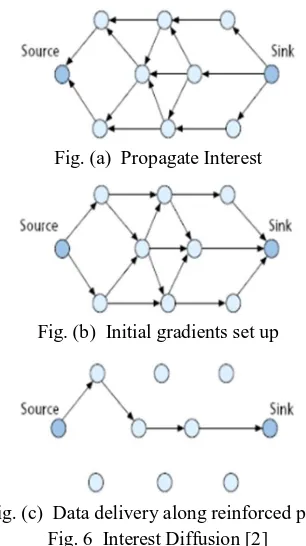
Directed diffusion involves 4 elements: interests, data messages, gradients, and reinforcements. Interest is like a query or an interrogation that specifies what the inquirer wants. In directed diffusion, this interest is present in a form of Attribute-Value pair. Gradient is a reply link towards the neighboring node from where the query is received. Reinforcement is the path selected by the information containing node which the data has to take to reach the base station in order to satisfy its query. The three process DD protocol is shown in Fig. 6.
Fig. (a) Propagate Interest
Fig. (b) Initial gradients set up
Fig. (c) Data delivery along reinforced path Fig. 6 Interest Diffusion [2]
For each active sensing work, the base station periodically sends messages to each neighbour. The message is then propagated to the whole network as an interest for a named particular data. As mentioned, interest is sent in the form of attribute-value pair. There are typically four attribute types- Type, Interval, Duration, and Field. Their corresponding values are sent in the form of a pair. Flooding is done in order to identify if any node contains any information according to the query/interest injected.
Nodes following directed diffusion maintain an interest cache containing entries for each interest it can give. The interest cache contains fields like timestamp field, multiple gradient fields for each neighbour, and a duration field. The timestamp field holds the timestamp of the former matching interest received. Gradient field cites both the data rate and the route, which the data has to follow. As soon as a node receives an interest, it checks if that interest occurs in the cache. If no match exists, it creates an interest entry. And then from the received interest information, it then fills up the parameters of the newly entered interest field. If a match exists, the timestamp and duration fields of the matching entry are updated by the node. Although there exists a much more exploratory process and condition regarding gradients and path, the above-mentioned method is quite simple and has the following advantages:
a) Small delay is experienced. The path reinforced is the shortest one.
b) Experiences much less traffic than flooding.
c) This protocol is robust to failed path.
d) Each node can do aggregation and caching.
[image:7.595.239.392.229.502.2]©IJRASET: All Rights are Reserved
1751
a) The nodes involved in the shortest path, drain their energy quickly in comparison with the other nodes of the network, creating an imbalance of node lifetime.
b) Some extra overhead is added when matching interest queries to data.
c) In appropriate for continuous data transmission, like environmental monitoring.
In [6], it’s been concluded that DD can display substantial energy efficiency and DD mechanisms remain stable under the dynamics of networks mentioned in [6]. However, extreme attention has to be paid to the design of MAC layers of the sensor radios in order for DD protocol to run at its maximum potential.
7) Geographical and Energy Aware Routing (GEAR): Y. Yu, R. Govindan, and D. Estrin in the year 2001 presented a geography intelligent protocol named GEAR [7] which was complementary to DD. Geographic and Energy Aware Routing (GEAR) protocol is a technique which routes a data packet towards the appropriate region using conscious neighbour selection along with recursive geographic forwarding to disseminate the data packet inside the destination region.
Geographic Information System (GIS) is used by a system implementing GEAR protocol for finding the location of the sensor nodes present in the network [4]. It is an improvement to direct diffusion in a sense that it does not inject the interest into the whole network, rather it concentrates only towards a certain region, thus restricting the number of interests.
[image:8.595.214.405.328.513.2]Fig.7 demonstrates the basic working of forwarding technique used in GEAR. MH is the message holder node and around it, has 5 neighbouring nodes. Amongst them, node D is the nearest to the destination node and hence, it is used for the next hop.
Fig. 7 Geographical routing forwarding [2]
8) GEAR Protocol Mandates The Nodes To Store Two Types Of Cost, For Reaching Its Destination a) Estimated cost- It is a combination of residual energy and distance to destination.
b) Learning cost- It is a modified estimated cost and it accounts the routing around holes in the network.
When a node does not have any closer neighbours towards the target region, then one says that there occurs a hole. If there are no holes, the above mentioned two costs are equal. i.e. Estimated cost=Learned cost.
9) GEAR Protocol Works In Two Phases
a) Phase I: Forwarding packets towards the region.
After receiving a data packet, the node inspects to see if there exists any neighbour who is closer to the target region than itself. The data packet is transferred if such node exists there. If more than one node exists, then the nearest to the target neighbour is selected as the next hop. If all of them are farther than that node itself, then it means that a hole has been encountered by that node. When this problem arises, one of the neighbour is picked up for forwarding the packet, based on the learning cost function.
b) Phase II: Forwarding the packets within the region.
©IJRASET: All Rights are Reserved
1752
10) GEAR protocol has the following advantages:
a) Conserves more energy than any other routing technique.
b) The rest of the network can still communicate even if the given traffic pairs are partitioned.
c) Concentrates on a specific region, hence the number of interest queries are minimized.
d) Can even work in regions of non-uniform traffic distribution.
e) Control overhead is relatively smaller in GEAR.
11) GEAR protocol has the following disadvantages:
a) It shows limited scalability
b) It requires limited or no mobility of sensor nodes.
GEAR involves the knowledge of geographic knowledge of every node. It was first proposed in [7], in the improvement to Greedy Perimeter Stateless Routing (GPSR). In [7], it’s been concluded that GEAR performs better than GPSR as GEAR delivers around 70%-80% more packets in cases of uneven traffic distributions. In even traffic distributions, this data is around 25%-35% more packets.
[image:9.595.57.541.322.489.2]Comparative analysis of all the routing protocols which have been detailed above are mentioned in Table 1, describing their different properties.
TABLE I: Comparative study of different routing protocols [1] [2] [3] [5] [6] [7]
III. SYSTEMMODEL
The simulation of LEACH protocol for WSN was performed using MATLAB-2017a. The code written is for a small region, or we can say, a small part of a big network. It can be further extended for the whole network. In this, the order of nodes, eligible to b ecome a cluster head is calculated beforehand. Afterwards, the nodes are plotted in a graph like manner showing the cluster head and the direction of data transmission.
A. Unique coordinates of the nodes were found out considering an area of (10x10) unit.
B. Initialized the LEACH formula variables viz. r and P.
C. Formulated T(n) and a random number (say, temprandom) was generated for the current round for that specific node.
D. Comparison was made between T(n) and that random number according to: temprandom<T, taking into the consideration a scenario wherein this comparison may result into false every time for that whole round and a step back must be taken to run that round again.
E. Distance between the nodes with one another was found out and arranged into a square matrix form.
F. All the nodes are given 100% energy.
G. A loop is run in which one by one cluster heads are picked up.
H. Using the cluster heads node number, a new square matrix is created based on distances between that cluster head and the other nodes.
I. A directed graph is constructed using that newly made square matrix.
J. Using a nested loop, under the condition that no node should be allowed to become a cluster head if its energy falls below 34%; energy of all the nodes including the cluster head are decreased by a factor of 0.5 and the energy of the cluster head is additionally decreased by a factor of 0.5 again. This makes the total decrement of cluster head energy by 1 as it has some additional tasks to perform.
Protocol Classificatio n Mobility of BS Power Manage ment Network Lifetime Scalabilit y Resource Awareness Data Aggrega tion Query Based Multip ath
Flooding Proactive/
Flat
Fixed Limited Average Limited Yes No No Yes
SPIN Proactive/
Flat
Supported Limited Good Limited Yes Yes Yes Yes
LEACH Clustering Fixed Maximu
m
Very Good Good Yes No No No
PEGASIS Reactive/
Clustering
Fixed Maximu
m
Very God Good Yes Yes No No
Directed Diffusion
Proactive / Flat
Limited Limited Good Limited Yes Yes Yes Yes
©IJRASET: All Rights are Reserved
1753
K. The directed graph made above was plotted and a pause of 5 second was taken.
L. When the loop increments, the next node in the list is taken out (as in step 7) and appointed as next cluster head. The whole process after step 8 is into run again.
Another simulation was done - on the basic direct routing protocol, in which all the nodes have the responsibility to sense as well as transmit the results directly to the base station in a single hop. It was coded in similarity with the simulation of LEACH protocol code. In this, nodes are randomly placed around a base station. Closer the node, the lesser energy it has to dissipate. Hence, it is all a play of distance of the nodes from the base station. Its algorithm is as follows:
1) The program of LEACH protocol was run and the random coordinate pairs it had generated, is fed as variables to this program to ensure that same network configuration could be achieved.
2) Base station is placed at (5,5) and the distances from each coordinate pair to it is found out and saved.
3) A directed graph is constructed using all the nodes and the base station.
4) All nodes are given 100% energy.
5) Energy from the nodes are decreased according to the following criteria:
a) If the distance is less than 2 then decrease 0.5% energy.
b) If the distance is greater than 2 and less than 4 (inclusive) then decrease 1% energy.
c) If the distance is greater than 4 and less than 6 (inclusive) then decrease 1.5% energy.
d) If the distance is greater than 6 and less than 8 (inclusive) then decrease 2% energy.
6) A pause of 5 second was applied, similar to that in LEACH protocol code.
7) Step 5 is repeated until at least one node drains out all of its energy.
IV. SIMULATIONRESULTS
The detailed results of the simulation performed on MATLAB-R2017a have been compiled in Table 2, which shows the order and the time for which the nodes have been designated as cluster heads.
TABLE 2 Simulation Results of LEACH protocol
A. Simulation of LEACH protocol:
Number of sensor nodes: 10
Total lifetime= 683.5184 second or 11.3920 minute.
Node numbers 7 & 8 were not eligible to be cluster head as by the time their turn came, their energy was already below the threshold of 34%.
B. Simulation Of Basic Direct Routing Protocol
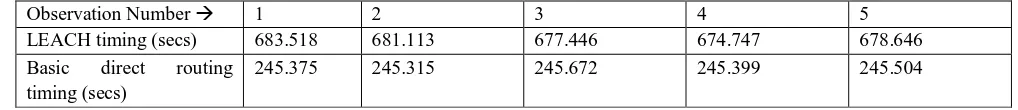
Simulation of basic direct routing protocol was carried out 5 times in a similar manner. Its total run time was compared with the LEACH protocols run time, which was also executed 5 times. The results been tabulated in Table 3.
[image:10.595.41.550.643.698.2]Number of observations: 5
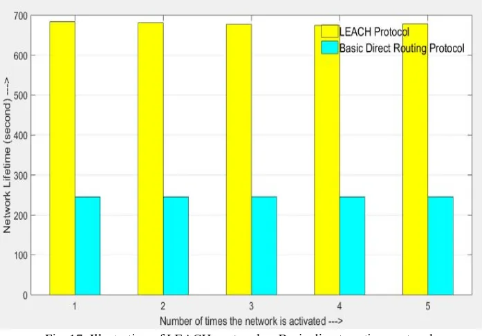
TABLE 3 Comparative simulation results of LEACH and basic direct routing protocol Observation Number 1 2 3 4 5 LEACH timing (secs) 683.518 681.113 677.446 674.747 678.646 Basic direct routing
timing (secs)
245.375 245.315 245.672 245.399 245.504
Average value of LEACH timing: 679.094 second.
Average value of basic direct routing timing: 245.453 second.
It’s inferred that LEACH protocol has 2.7667 times more run time than basic direct routing protocol. CH order
2 1 4 3 9 10 5 6 7 8 Time(sec) 345.318320 168.829458 87.330267 40.996420 20.565051 10.218364 5.129263 5.131196 - -
Energy left (%)
©IJRASET: All Rights are Reserved
1754
Fig. 8. Plotting results of LEACH protocol and basic direct routing protocol from Table 3
V. SIMULATEDNETWORKDIAGRAMS
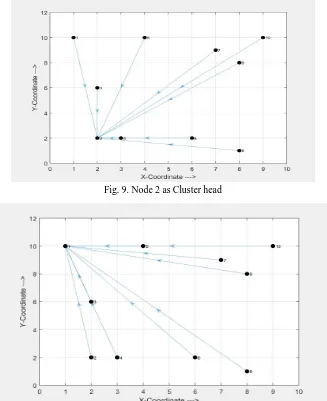
[image:11.595.133.464.111.250.2]Executed on MATLAB-R2017a software, the output network diagrams are shown from Fig. 9 to Fig. 16. These network diagrams depict the ordered designated cluster heads, different nodes and the flow of sensor collected data, which are separate nodes towards the cluster head at that particular time.
Fig. 9. Node 2 as Cluster head
[image:11.595.135.462.324.725.2]©IJRASET: All Rights are Reserved
1755
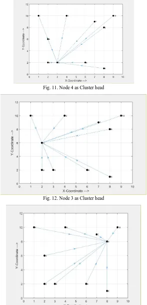
Fig. 11. Node 4 as Cluster head
Fig. 12. Node 3 as Cluster head
©IJRASET: All Rights are Reserved
1756
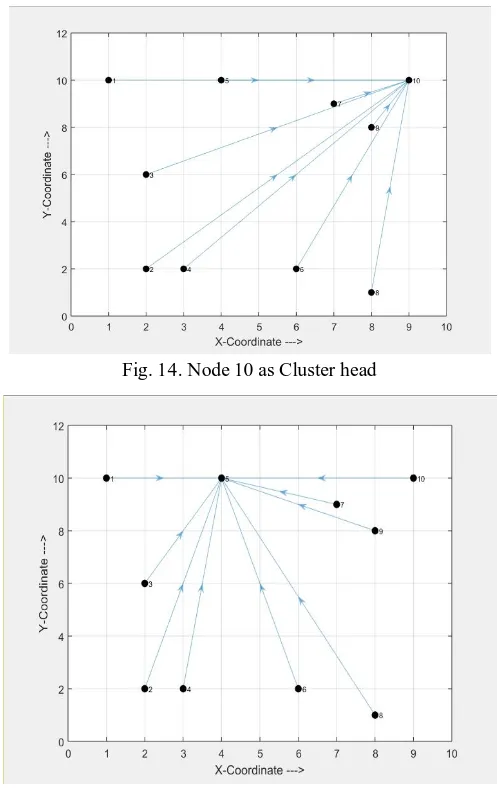
[image:13.595.155.441.479.720.2]Fig. 14. Node 10 as Cluster head
Fig. 15. Node 5 as Cluster head
©IJRASET: All Rights are Reserved
1757
VI. ANALYSISOFTHERESULTS
A. In this paper, we have described the results of simulation of LEACH protocol and compared it with the Basic direct routing protocol.
B. Network configuration in LEACH protocol may change (due to random selection of coordinate pairs), therefore network lifetime varies a little.
[image:14.595.125.475.207.450.2]C. The lifetime of LEACH was found to be much greater than other conventional protocols like flooding and simple transmission technique. This can be visualized from the comparison bar chart shown in Fig. 17.
Fig. 17. Illustration of LEACH protocol vs Basic direct routing protocol
D. Network lifetime of LEACH was approximately 3 times that of basic direct routing protocol. Furthermore, in[1], it has been is claimed that full LEACH has approximately 8 times more network lifetime than earlier methods.
E. LEACH protocol has taken the responsibility of being a Cluster Head between the cluster member nodes which eventually led to the efficient use of the network energy and longevity of the network lifetime.
VII. CONCLUSIONS
Simulation of LEACH protocol using MATLAB-R2017a and its comparison with the basic direct routing protocol was done and by the results obtained, it can be successfully concluded that under LEACH protocol, the lifetime of the network has increased because it saves network energy, by distributing the load to all the nodes at different point of time. Its MAC based features and TDMA supporting capabilities, together with the concept of clustering hierarchy paves a way for fast communication & energy conservation, hence resulting in longevity of the network lifetime. As LEACH is completely distributed, it entails no direction from the base station and the nodes require no information of the whole network. So, it does not require nodes to burden themselves with sensing, aggregating and sending it to the base station.
It is also concluded that if any node dies out due to any technical failure then it does not affect that network very much in LEACH protocol; because the whole network gets divided into new clusters, each time the responsibility of a cluster head gets changed. Although, it has a serious implication that dying node should not be a cluster head as then that whole cluster will become useless.
VIII. ACKNOWLEDGMENT
©IJRASET: All Rights are Reserved
1758
REFERENCES
[1] Heinzelman, W.R., Chandrakasan, A., and Balakrishnan, H. (2000) Energy-Efficient Communication Protocol for Wireless Microsensor Networks. Proceedings of the Hawaii Intl Conference on System Sciences; Maui, Hawaii, Jan 4-7, pp.10.
[2] Sohraby, K., Minoli D. and Znati T. (2007) Wireless Sensor Networks: Technology, Protocols, and Applications. [Routing Protocols for Wireless Sensor Networks], John Wiley & Sons, Inc., New Jersey, U.S.A., pp. [197-220.].
[3] Al-Karaki, J.N. and Kamal, A.E. (2009) Routing Techniques in Wireless Sensor Networks: A Survey. IEEE Wireless Communications, 03 (06),pp. 612–627.
DOI: 10.1109/MWC.2004.1368893
[4] Bhattacharyya, D., Kim, T., and Pal, S. (2010) A Comparative Study of Wireless Sensor Networks and their Routing Protocols. Sensors, 10,pp. 10506-10523.
DOI:10.3390/s101210506
[5] Tandel, R.I. (2016) Leach Protocol in Wireless Sensor Network: A Survey. Intl. Jl. Of Computer Science and Infor. Technologies, 07 (04),pp. 1894-1896. [6] Meghanathan, N. (2009) Use of Tree Traversal Algorithms for Chain Formation in the PEGASIS Data Gathering Protocol for Wireless Sensor Networks. KSII
Transactions of Internet and Information Systems, 03 (06), pp. 612–627. DOI: 10.3837/tiis.2009.06.003
[7] Yu, Y., Govindan, R. and Estrin, D. (2001) Geographical and Energy Aware Routing: a recursive data dissemination protocol for wireless sensor networks.
https://pdfs.semanticscholar.org/11ca/e1f847d741052bffba9af8d9fbd39973fd94.pdf
[8] Patil, R. and Padiya, P. (2016) An Efficient Method for Selection of Cluster Heads Based Upon the Neighbourhood Characteristics in WSN. Intl. Jl. Of Adv. Research in Computer Sci. and Software Engg., 06 (04), pp. 250–254.
![Fig. 3 Basic SPIN protocol operations [2]](https://thumb-us.123doks.com/thumbv2/123dok_us/1241227.650121/3.595.203.419.442.595/fig-basic-spin-protocol-operations.webp)
![Fig. 7 Geographical routing forwarding [2]](https://thumb-us.123doks.com/thumbv2/123dok_us/1241227.650121/8.595.214.405.328.513/fig-geographical-routing-forwarding.webp)
![TABLE I: Comparative study of different routing protocols [1] [2] [3] [5] [6] [7]](https://thumb-us.123doks.com/thumbv2/123dok_us/1241227.650121/9.595.57.541.322.489/table-i-comparative-study-different-routing-protocols.webp)